From Structural Optimization Results to Parametric CAD Modeling—Automated, Skeletonization-Based Truss Recognition

Abstract

This paper presents an automated, skeletonization-based feature recognition system designed for use with biomimetic structural optimization results. It enables importing optimization results back to the CAD system as a set of parameterized geometries. The system decomposes the output of the structural optimization system into a set of simple CAD features, cylinders and spheres, enabling continuation of mechanical design workflow using native CAD representation. The system was designed to work in a fully automated mode accepting 3D objects as an input. The system uses mesh skeletonization to generate an initial solution which is refined using an evolutionary algorithm for the 3D geometry reconstruction. The system is designed as the last step of structural optimization. Applied for industrial use, it preserves unique features of this approach, such as excluding parts of the domain from optimization. The biomimetic topology optimization was used for structural optimization for all presented examples. The proposed algorithm is demonstrated using two cases: well-recognized cantilever beam optimization and industrial application of the structural optimization. For both cases, resultant geometry stress distribution is provided and analyzed.

1. Introduction

Design of lightweight structures, which have both low mass and good mechanical properties, became a crucial part of the mechanical design process. It is achieved not only by using advanced lightweight materials, but mainly by using the advanced design process. The leading industrial approach is the use of structural optimization to design both the stiffest and lightweight design. Combined with Additive Manufacturing techniques [1,2,3], structural optimization is an excellent method for achieving solutions greatly exceeding what is possible to create using traditional techniques of design and manufacturing.

Structural optimization software, by design, is based on the structural analysis numerical methods. Those methods, with the Finite Elements Method as the dominant approach, require discretization of the analyzed area. This leads to discretized results of structural optimization—a surface or volumetric finite element mesh. Additive manufacturing production methods may reduce the post-processing of structural optimization results to the mesh surface smoothing only. In many practical cases, in particular when after optimization further design requires a parametric model, there is a need for transferring structural optimization results to the CAD system. This requires building a parametric model.

This paper describes the approach of building CAD parametric models using cylindrical structural elements—the result is truss. The entry point for the presented approach is an output mesh obtained by optimization performed using the biometric approach to structural optimization [4,5,6] which utilizes a new paradigm of ultralight constructions considering material properties and enables solving optimization problems for multiple load scenarios. The presented features recognition algorithm works properly for truss structures appearing in a broad variety of structural optimization results. The algorithm is based on the skeletonization of a mesh directly obtained from the biomimetic structural optimization system. The skeleton is used to determine the topology of the initial solution, which is refined using a heuristic optimization approach. The final solution is transformed into a parametric model, which can be imported into the CAD system. An important feature of the presented approach is a fully automated method of operation. The proper operation of the reconstruction algorithm is proved using typical topology optimization problems, which are well described in the literature. Detailed analysis is performed using two case studies. First is an optimized cantilever bar and second is an industrial application—the optimization of a box corner. For both case studies, structural analysis was performed and the results are discussed. The approach is validated and future directions of research are proposed.

The efficiency of the algorithm is demonstrated in the second case study—the industrial use of biomimetic optimization in the BioniAMoto project. The aim of the BioniAMoto project is to develop a cost-effective method for manufacturing lightweight and efficient structural nodes for the automotive industry using additive manufacturing (AM) technologies and structural optimization. The project aims to create a new concept for manufacturing 3D structural nodes for vehicle frames using topology-optimized aluminum alloys that are joined together with readily available and commonly used extruded profiles. One of the parts manufactured as a part of the project is an aluminum box corner used in truck cars. The use of the presented approach enables the conversion of the results of the structural optimization to the parametric model, which simplifies the post-processing steps required to prepare the model for the manufacturing process. Two additive manufacturing processes are considered. The direct method, Laser Metal Powder Bed Fusion (LM-PBF) technology, uses a laser beam to fuse metal powder. The second approach is an indirect method using Laser Polymer Powder Bed Fusion (LP-PBF) technology to create the initial model, which is used, in turn, to create the mold used for the manufacturing using Injection Molding. Both approaches have limitations that require model processing before manufacturing. One example is the minimal element thickness imposed by both approaches. In the direct method, the limiting factor is the thermal stress, in the indirect method—the molten metal flow properties during the casting process. The use of parametric models in CAD software allows adjustments to the optimized model to consider those phenomena.

Structural optimization is used as one of many steps in the Additive Manufacturing design workflow, which starts with product planning and ends at product validation [7]. The optimized part is further processed in CAD software to post-process it and prepare for manufacturing [8]. There are a lot of techniques for the post-processing of 2D structural optimization results, mostly based on image recognition techniques such as Hough transform [9], morphological processing [10] or features mapping [11,12]. The selection of post-processing techniques in a 3D domain, due to the greatly increased number of topological complexities [13], is limited. Techniques are based on removing material from the initial full domain, by matching pre-defined 2D shape templates [14] or by matching machining features using dedicated algorithms [15] or machine learning [16,17]. The skeletonization of structural optimization results enables tracing models with cubic B-splines, either as a manual, computer-aided process [18] or as a fully automated process [19]. Approaches gaining popularity with Additive Manufacturing [20] are based on mesh processing such as smoothing [21] without converting the results to a CAD model or converting the results to a CAD model as a watertight shell [22].

The goal of the used structural optimization algorithm is to equalize the surface strain energy density distribution. Topology with uniform distribution under a load has both maximal stiffness and minimal mass [6]. In nature, this phenomenon is observed in trabecular bones. Bone tissue is constantly remodeled as it reacts to the external stress by growing in areas with high stress concentration and removing where it is not required [23]. This bio-mechanic process is simulated in the structural optimization process to equalize surface strain energy density in the optimized model. The volumetric mesh generator integrated in the structural optimization system works using custom modification of the marching cubes algorithm [24] optimized for use with FEM systems. The produced mesh is free of topology errors such as non-manifold surfaces [25] and is watertight [22]. This is the distinctive feature of an underlying approach compared to the Solid Isotropic Material with Penalization (SIMP) method [26,27,28]. The SIMP algorithm requires a dedicated discretization step with the desired mesh volume as a parameter. The biomimetic approach operates by modifying a mesh directly, starting from an existing design, which allows improving the existing designs [29] and uses the material mechanical properties to determine the maximal allowed stress. Hence, it is possible to use the output of structural optimization directly in a proposed feature recognition algorithm.

2. Materials and Methods

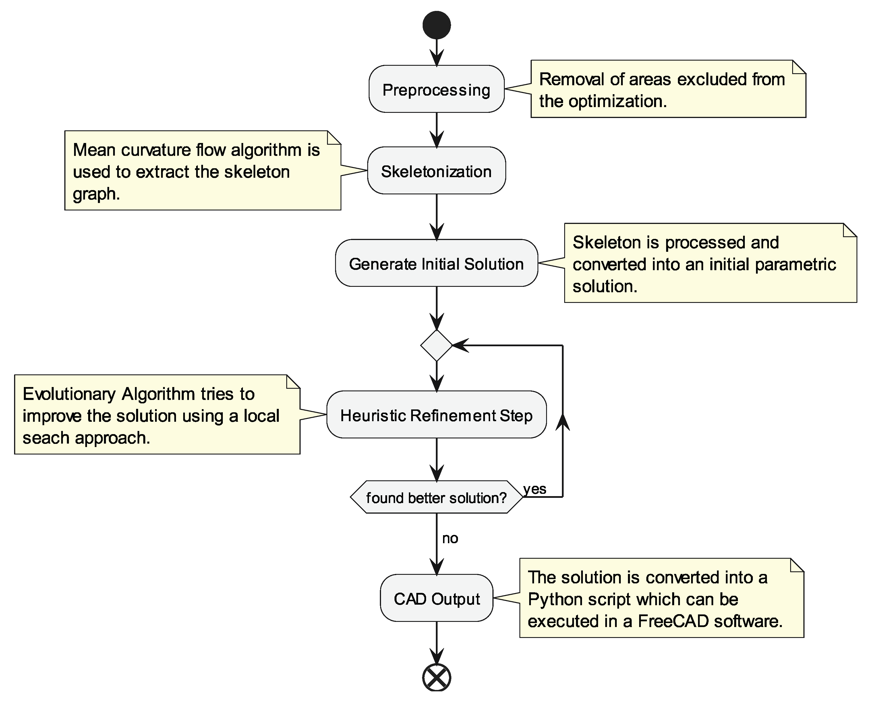
The recognition algorithm uses few distinctive steps, as seen in Figure 1. The input of the algorithm is both the input data and the resulting mesh of the structural optimization system. The sample input for the algorithm, created using FreeCAD software, is provided in Figure 2. The first step is the extraction of the area of interest. The result of the structural optimization contains the whole optimization domain, which may include areas excluded from optimization. Those areas are both positive and negative exclusions, that is, areas which contain material that must not be removed, such as attachment points and areas which must not contain material, such as holes for screws or those occupied by elements that are not a subject of the optimization. Areas which contain material and are excluded from optimization are removed from the input mesh—a parametric model for those already exists as an input for the algorithm so there is no need to re-import it to the CAD system. The definition of areas excluded from optimization is taken from the input of the structural optimization system. The second step is skeletonization. The mesh skeleton is obtained, processed and used in the next step to generate the initial solution. The solution is then iteratively refined using a heuristic optimization approach. The refined solution is converted to a format that can be imported to the CAD system—FreeCAD.

2.1. Preprocessing

The output of the structural optimization is a triangulated mesh, ready to use by the truss recognition algorithm. The first step is the removal of areas defined in the optimization task as being excluded from the optimization. Those areas, in practice, contain attachment points that must be preserved throughout the whole process and are not subject to either structural optimization or feature recognition.

The removal of the excluded areas is performed by the structural optimization software by generating a mesh consisting of all the points that do not belong to the excluded areas. Using the same generator as used for the structural optimization results is important to preserve the mesh points density, which is also important in the next steps of the algorithm. A constant mesh vertex density improves the reliability of the mesh skeletonization and is required later by the refinement step to calculate the score of each candidate. Initially, an algorithm provided by CGAL library was used, but re-meshing applied by it altered the mesh density which, in turn, decreased the quality of the next steps of the feature recognition process. A comparison of both approaches is illustrated in Figure 3.

2.2. Skeletonization

The mesh skeletonization is performed using the mean curvature skeleton algorithm [30]. Unlike other approaches, such as the algorithm used in [18], the mean curvature skeleton output is a graph representing the mesh skeleton and there is no need for additional processing. The skeletonization algorithm works really well with a biomimetic optimization output despite the jagged surface of the resulting mesh. There are no disconnected areas or undesirable skeleton curves. Such artifacts are often presented in skeletons obtained by techniques based on morphological filtering, as seen in [10,31]. As shown during preprocessing, the skeletonization algorithm is sensitive to mesh density. The resolution of the skeletonization can be increased by increasing the mesh density using a loop subdivision algorithm [32]. The performed tests showed no improvement of the initial solution’s quality when using higher resolution meshes, but the skeletonization time increased greatly. Hence, the mesh returned by a mesh generator from a structural optimization system is used as-is for the skeletonization algorithm input. Sample meshes with matching skeletons are shown in Figure 4.

There was no attempt to improve the skeleton alignment inside the mesh. Although this would improve the initial solution quality, for proof of concept work, this part is considered redundant. The refinement step, performed next, should yield similar results.

2.3. Skeleton Processing

The graph representing the skeletonized mesh is processed to obtain the initial solution. This process has a single configuration variable: the minimum path length. In the first step of the process, all paths between the graph’s loose nodes (with a single edge) or intersection nodes (with more than two edges) are calculated. Those paths are either replaced with single edges, or, if the path curvature is high enough, with a series of edges approximating the path. A biomimetic approach used as an input of the recognition algorithm yields a porous and unstable structure in areas where the mesh resolution is insufficient to represent the fine microstructure present in the analytical solution, as shown in Figure 5. This phenomenon justifies filtering out such porous structures in the initial solution. Hence, all edges shorter than the given minimum path length are collapsed. This also enables some degree of solution resolution control—a high value of minimum path length simplifies topology by collapsing the fine details. Sample data illustrating the whole process are illustrated in Figure 6. Finally, the graph obtained this way is converted into the initial solution by assigning the default radius to each graph edge.

2.4. Heuristic Refinement

The initial solution obtained from the skeletonized and processed output needs further refinement. This refinement is performed using an evolutionary algorithm that iteratively improves the solution. Unlike the biomimetic structural optimization, the iterative algorithm is based on a theoretical mathematical model proved to be valid, and the proposed solution is heuristic and created experimentally. The algorithm is designed to be fast, and the trade-off is reduced accuracy.

The evolutionary algorithm requires the definition of the Fitness Function to calculate a score for each candidate and select the best one. The Fitness Function must be quick to compute and at the same time accurate to enable visiting many candidates in a short time. The optimal solution of a feature recognition algorithm is a set of features that completely fill the volume of input data and do not exceed it. Scoring based on volume requires the time-consuming operation of intersecting the input mesh with the scored solution to find differences. The optimization of this approach uses a mesh discretized using a slice-based approach and comparing discrete sets of points. This approach has $O\left(n^3\right)$ complexity, so a more efficient but less precise approach was used. As the algorithm operates on the surface, the not-volumetric, mesh, surface-based approach was also used for the Fitness Function. Two sets of points are calculated: control points and guide points. Control points are points on a mesh surface that are used to determine how close a solution’s surface is to the input surface. A set of guide points is obtained by the morphology dilation of the input mesh. The size of the dilation is an input parameter of the algorithm. Details of the mesh surrounded by the guide points are shown in Figure 7.

The Fitness Function is calculated for a solution consisting of the set of elements, E, the given set of control mesh points, P, and guide points, G. $Surface\_distance(p,e)$ is a function that returns the Euclidean distance between element e’s surface and point p. $is\_inside(p,e)$ is 1 if the point p is inside geometry g, and is otherwise 0.

$$S_{positive}=\sum _{p\in P}\underset{\forall e\in E}{min} surface\_distance{(p,e)}^2$$

(1)

$$S_{negative}=\sum _{g\in G}\underset{\forall e\in E}{min}-{(surface\_distance(g,e)\ast is\_inside(g,e))}^2$$

(2)

$$Fitness=\alpha S_{positive}+\beta S_{negative}$$

(3)

The solution is scored positively for the matching input surface and is penalized for enveloping guide points and taking more volume than required. Both positive and negative scores are aggregated using weights, $\alpha$ and $\beta$, used to equalize imbalances in the size of two sets. For tests, $\alpha =1$ and $\beta =50$ were used. To increase performance, for each evolutionary algorithm iteration, a subset of both sets was generated. A total of 20% of mesh points and 4% of guide points were randomly selected. The size of the guide set is five times smaller than the size of the control points so, effectively, the weight of the negative score was ten times higher than the positive. It is important to note that this approach works well because the input mesh, obtained from the mesh generator, which is part of the structural optimization algorithm, is built from regularly spaced elements. Without this feature, an extra algorithm step would be required to ensure that the mesh vertices are equally spaced and uniformly cover the mesh surface.

The evolutionary algorithm works iteratively, creating a set of candidates using random sampling of a solution neighborhood space using two available operations. In the descriptions, $\mathcal{N}(\mu ,{\sigma }^2)$ is the function returning the normally distributed random value. The first operation is moving one randomly taken solution graph node by random vector

$$v=\left[\begin{array}{c}\mathcal{N}(0,{\sigma }_{dir}^2)\\ \mathcal{N}(0,{\sigma }_{dir}^2)\\ \mathcal{N}(0,{\sigma }_{dir}^2)\end{array}\right]$$

(4)

${\sigma }_{dir}$ is a parameter of an algorithm. Second is the changing radius of the random cylinder by $\mathcal{N}(0,{\sigma }_r^2)$. ${\sigma }_r$ is a parameter of an algorithm. Each candidate solution is created by applying random operations 1 to 5 times. A moving graph node has twice the probability of being applied than a changing radius. All candidate solutions are scored using a Fitness Function and the best one is returned. A single iteration visits 5000 solutions. The stop criterion is exceeding the pre-set number of iterations or there being no improvement after 20 iterations.

Although the current implementation reconstructs the optimized object using cylinders, the refinement step was designed to work with any part. A framework built in this way allows an easy change of structural element to, i.e. square beam, or the use of curved elements. The cylinder was chosen for proof of concept work because it has fewer degrees of freedom than other structural elements.

2.5. Postprocessing and CAD Integration

The refined mesh is converted into a format that can be imported into CAD software. FreeCAD was selected because of a non-proprietary license and extensive documentation. The results are converted into a Python script that uses FreeCAD’s API [33] to create parts consisting of cylinders.

Additionally, the export script creates spheres at each node to ensure a proper connection between cylinders, as shown in Figure 8. The radius of each sphere is 110% of the biggest radius of the element connected to the node. The extra margin was added to avoid numeric errors reported by CAD software when fusing elements with a similar radius to produce the final mesh. Note that those spheres are only added in the final step and are not part of the ’main’ geometry. Hence, to simplify the calculation of the Fitness Function, it was decided to ignore those extra parts during the refinement step, despite the fact that they contribute to the overall volume and mass of the model.

An alternative output is the implementation of producing a set of IGES (Initial Graphics Exchange Specification) format files, which provides a vendor-neutral way of importing object information into CAD systems.

2.6. Solution Verification—Methodology

The Fitness Function defined for the evolutionary algorithm used during refinement step cannot be used to measure the quality of the solution. The Fitness Function is used to heuristically compare solution candidates but does not have the information if the mechanical properties of the solution match ones of the input mesh. Solution verification is performed by computing the same measures for two objects—the structural optimization result, which is also an input for the feature recognition system, and the reconstructed parametric solution, exported from the CAD system as an STL mesh.

The first compared measure is the total mass of an object. Objects reconstructed in CAD should not have a bigger mass than the source objects, so the mass of the object after the structural optimization is compared with the mass of the reconstructed object exported from the CAD system. The mass is calculated using the density of the material and the volume of the mesh. The density is an input parameter of the optimization process and the volume is calculated using a volumetric mesh generator, which is part of the structural optimization system. The volume of all constituent mesh cells is summed to get the total mesh volume.

The surface energy value, which is equalized during structural optimization, is selected in such a way that the von Mises stress does not exceed the critical value. Fulfilling the von Mises yield criterion guarantees structural integrity under the load of the optimization results. A second test is performed to prove that the von Mises stress in a reconstructed object does not exceed the maximum von Mises stress present in the structural optimization results. To obtain a stress distribution, the object is exported from CAD and loaded back into the structural optimization system. The exported surface mesh is first converted into a volumetric mesh and then into Finite Elements Method input data. A static elasticity calculation is performed using FrontISTR software [34,35]. The maximal value of the von Mises stress is obtained and the stress distribution is analyzed. Together with the values of the von Mises stress, the displacement data were obtained. Using mesh displacements, the maximum deflection under load is calculated. Despite it providing no extra information compared to von Mises stress, the maximum deflection is a value often used in engineering analysis, so it is also presented. In case of multiple load scenarios, tests must be performed for each scenario independently.

The presented solution verification has been performed for both cases described below.

3. Results

3.1. Comparison with the Literature

Process results were tested using two structural optimization solutions for which analysis has been carried out in the past. First is the output of Bremicker’s cantilever beam results using the homogenization method [31]. The parametric model for a 2D solution was provided by [9,10,31]. The obtained 2D result was extruded into a 3D mesh. The size of a bounding box of the mesh was 230 mm × 144 mm × 18 mm. The input mesh, skeletonized output and initial and refined solutions are visible in Figure 9. The obtained skeleton is noticeably higher quality than the one presented in the original work and allows capturing of the solution’s topology. The second test is the cantilever beam provided in [9] and also analyzed in [10]. A similar but not exactly the same part was analyzed in [12,19]. Again, the 2D mesh was extruded and the size of a bounding box of the mesh was 600 mm × 162 mm × 25 mm. Results are illustrated in Figure 10, demonstrating the proper operation of the feature recognition system. Visual inspection, as demonstrated in Figure 11, indicates the proper operation of the algorithm. The cited research did not perform stress analysis; hence, it was not performed for the obtained parametric models.

3.2. Case Study 1—Cantilever Bar Bending

The first case is the optimization of loading the steel bar. This is a standard example of topology optimization and this problem has been solved analytically [26]. The structural optimization algorithm is used to obtain the input for the feature recognition algorithm, which was proved to provide the optimal solution [4]. It is important to note that the examples in the comparison with the literature were performed on extruded 2D optimization results. This case study is performed for a true 3D object with an optimization domain with one dimension restricted. The input for the optimization was created in CAD software using the following parts: optimization domain—box 20 mm × 500 mm × 1000 mm; bar to be optimized—box 20 mm × 20 mm × 1000 mm centered inside domain; support area—box 1000 mm × 1000 mm × 2 mm; stressed area—box 20 mm × 20 mm × 2 mm. All parts modeled in CAD are visible in Figure 12. The parts for use with the structural optimization system were exported as STL files. The material of the optimized model was steel with $\nu =0.28$, $E=200\times {10}^9$ Pa, $\rho =7800$ kg/m${}^3$. The yield strength for the material was assumed to be $250\times {10}^6$ Pa. The bar was stressed with a force of 40 kN perpendicular to the axis. For this, a test factor of safety = 3 was assumed and the max allowed von Mises stress was set to $80\times {10}^6$ Pa.

Structural optimization was run for 300 iterations. It is important to note that this case study has been prepared to compare results with examples widely used as a benchmark for structural optimization and the implementation of the results is not possible. A shear force of 40 kN is applied to the area of 20 mm × 20 mm and this alone would cause structural failure.

The mesh from the structural optimization was directly used as an input for the feature recognition system. Refinement was run with the parameters displayed in

Table 1. Parameters of feature recognition algorithm used in Case Study 1.

Parameter	Value
Initial cylinder radius	10 mm
Minimal Initial Element Size	40 mm
Population	5000
Node Move Standard Deviation	5.0 mm
Radius Change Standard Deviation	1.0 mm

. The refinement progress is shown in Figure 13.

The result of the feature recognition algorithms was imported into the CAD system and exported as an STL file, which was used in the solution verification (Figure 14). The numeric results are in

Table 2. Comparison of mass and stress values for input mesh and parametric model for Case Study 1.

	Input Mesh	Parametric Model
Total Mass	18.41 kg	18.35 kg
Max von Mises stress on surface	$551\times {10}^6$ Pa	$436\times {10}^6$ Pa
Mean von Mises stress on surface	$55.7\times {10}^6$ Pa	$62.6\times {10}^6$ Pa
Max Deflection	2.008 mm	1.340 mm

. The boxplot of the surface von Mises stress is Figure 15. The reconstructed object is 0.3% lighter than the structural optimization result, so the algorithm produced an object of similar mass. The reconstructed object has a lower maximal surface von Mises stress and exhibits smaller deflection under load. The overall von Mises distribution is more concentrated (interquartile range $19.97\times {10}^6$ Pa in reconstructed vs. $52.67\times {10}^6$ Pa for reconstruction input), which suggests better distribution of load under stress in the reconstructed objects. This is because the compression/tension stresses dominate in this structure and the cylinder, which is the chosen structural element, carries those loads well. On the other hand, the von Mises stress is higher and a visual inspection of the FEM results shows excessive stress at the element connections (Figure 16). Those are the points where the bending moments concentrate. Disregarding the impossible load conditions, the implementation of the result would require manual strengthening of those points in CAD software to avoid structural failure.

3.3. Case Study 2—Box Corner

The second analyzed case study is a feature recognition run for the structural optimization of an aluminum box corner. The structural optimization has been performed as part of the mechanical design workflow. The manufacturing technique is 3D printing using the Powder Bed Fusion (PBF) technique. For manufacturing pre-processing, at the moment of this paper’s creation, surface smoothing is considered. The following case study has been performed to evaluate the reconstruction of a parametric model as a pre-processing step for use in this particular case. The structural optimization using aluminum ($\nu =0.33$, $E=70\times {10}^9$ Pa, $\rho =2800$ kg/m${}^3$) was performed with multiple (three) load scenarios. The maximum allowed von Mises stress was set to $70\times {10}^6$ Pa. The input geometries are shown in Figure 17. The boundary areas are color coded and used to describe the multiple load scenarios in

Table 3. Forces and support assignment to boundary areas for load cases in the structural optimization task. Refer to Figure 17 for color-coded boundary areas’ locations.

	Yellow Boundary	Blue Boundary	Red Boundary
Load Case 1	Force 200 N, vector Y = −1	Force 200 N, vector X = 1	support
Load Case 2	Force 200 N, vector Z = 1	support	Force 200 N, vector X = −1
Load Case 3	support	Force 200 N, vector Z = 1	Force 200 N, vector Y = −1

. The optimization was run for 200 steps and the results of the optimization are shown in Figure 18. The prototype manufactured for the initial evaluation is in Figure 19.

The mesh from the structural optimization was directly used as an input for the feature recognition system. Unlike in Case Study 1, this optimization problem contains areas excluded from optimization. Those areas were removed from the mesh in the pre-processing step. Refinement was run with the parameters displayed in

Table 4. Parameters of feature recognition algorithm used in Case Study 2.

Parameter	Value
Initial Cylinder Radius	1.0 mm
Minimal Initial Element Size	3.0 mm
Population	5000
Node Move Standard Deviation	0.2 mm
Radius Change Standard Deviation	0.2 mm

. The output from the feature recognition process steps is shown in Figure 20. Structural analysis was performed after the parametric model was obtained, and areas excluded from optimization were reattached to the reconstructed object in a CAD system. The altered mesh was exported from the CAD system in an STL format and used for the structural analysis. As the optimization problem contains three different load scenarios, the structural analysis was also performed three times, once for each load scenario.

Table 5. Comparison of mass and stress values for input mesh and parametric model for Case Study 2.

		Input Mesh	Parametric Model
	Mass	64.1 g	72.4 g
Load Case 1
	Max von Mises stress on surface	$141\times {10}^6$ Pa	$236\times {10}^6$ Pa
	Mean von Mises stress on surface	$23.1\times {10}^6$ Pa	$21.9\times {10}^6$ Pa
	Max Deflection at Force 1	0.82 mm	0.78 mm
	Max Deflection at Force 2	0.61 mm	0.62 mm
Load Case 2
	Max von Mises stress on surface	$178\times {10}^6$ Pa	$248\times {10}^6$ Pa
	Mean von Mises stress on surface	$19.98\times {10}^6$ Pa	$17.6\times {10}^6$ Pa
	Max Deflection at Force 1	0.73 mm	0.61 mm
	Max Deflection at Force 2	0.68 mm	1.0 mm
Load Case 3
	Max von Mises stress on surface	$263\times {10}^6$ Pa	$436\times {10}^6$ Pa
	Mean von Mises stress on surface	$28.3\times {10}^6$ Pa	$28.9\times {10}^6$ Pa
	Max Deflection at Force 1	1.6 mm	2.29 mm
	Max Deflection at Force 2	0.96 mm	1.28 mm

contains a summary of the analysis. Figure 21 shows the surface stress distribution for each load scenario, which are also presented as boxplots (Figure 22).

The reconstructed object exhibits both a higher overall mass and worse material properties. Although, for Load Case 1, the parametric model exhibits a lower mean stress and comparable deflection values. For Load Case 2 and Load Case 3, all analyzed measures exceed acceptable values. Details with areas exceeding the allowed surface von Mises stress are visible in Figure 23. Analysis shows that a cylindrical structural element, used to build the parametric model, is insufficient to represent the complex structure of the element optimized using the biomimetic approach. The surface stress exceeds the material’s yield strengths in a few different distinct cases: the attachment points to the boundary areas are insufficient, the connection between elements are too weak and the cylinders exhibit poor behavior under bending moments (Figure 24). On the other hand all those problems can be solved manually by engineers in CAD software based on the provided structural analysis results.

4. Discussion

Although there are multiple structural optimization methodologies, the challenge of a transition from a finite element mesh to parameterized model is always the same. Depending on the selected manufacturing method, it is possible to limit the optimization results processing to surface smoothing and continue the design process by relying on the manufacturing method preparation steps. The separation of the design optimization step and the manufacturing preparation step simplifies the overall manufacturing workflow but in practice is often insufficient—it is impossible to backtrack from the latter step and introduce adjustments other than direct operations on a mesh. The approach presented in the paper, coupled with the structural optimization process, allows for an interpretation procedure that uses a mesh generated by the discretization process, tailored for the finite elements method. Moreover, using a developed mesh generator, it is possible to adapt a feature recognition system to interpret results from any structural optimization system by remeshing the results. Extending the current implementation to allow for such operations is planned in the future.

The conversion of the structural optimization results back into parametric models is an important research area that is vital not only for the preparation of the manufacturing process, but also when the mechanical design process requires, after the structural optimization step, more design cycles based on parametric models in CAD systems. The presented solution meets this demand while providing another feature desired for industrialization—a fully automated process. In the context of the mechanical design process, the proposed solution shifts the paradigm of the structural optimization step. The structural optimization step no longer breaks the consistency of the overall design process by transforming the solution from the parametric form to a finite element mesh. The structural optimization coupled with automated feature recognition transforms a parametric model into an optimized parametric model. From the viewpoint of engineers involved in industrial design, the whole process is consistent and uses parameterized models that can be easily modified or adjusted end-to-end.

The described process is just a framework enabling further development. The main areas of improvement are as follows:

• Truss-based geometry was chosen because, compared to more complex geometries, it has fewer degrees of freedom to optimize, so the heuristic refinement process converges fast. The chosen structural elements are insufficient for structures with bending moments under load and there is a need for support of more complex geometries to properly capture the complexity of the input meshes. The proposed heuristic refinement step and the Fitness Function in particular work with solutions built out of any parameterized geometries. This makes it possible to apply the algorithm to any geometries produced by structural optimization algorithms, without the current limitation to trusses.
• The refinement process is heuristic; hence, the final solution may not meet the required mechanical properties. There is a need for research into the viability of adding an additional final refinement step where feedback from structural analysis is used to adjust the model.
• Heuristic refinement in this proof of concept work utilizes a random search approach. This process can be highly optimized. For example, adjusting positions of solution graph nodes is possible with the use of gradient descent methods.
• The initial topology, obtained from the processed mesh skeleton, is not changed during refinement. It is possible to enrich the heuristic refinement step with operations by changing the solution graph topology.
• The algorithm configuration, such as heuristic refinement parameters, should be replaced with values derived directly from input data, i.e. the initial solution’s cylinder radius can be automatically determined using the mean diameter of the input mesh structures.
• The presented approach is a fully automated parametrization procedure. On the other hand, when the manufacturing preparation requires increasing minimal thickness, for example, to decrease thermal stresses during the manufacturing process, a parametric model produced by the algorithm can be used to manually apply corrections. Those corrections are then fused back with the original mesh, preserving features that were not captured by the parametric model while improving the properties of the optimized mesh. Additional research is required to evaluate this approach for industrial use.

All the described improvement directions are currently under development in ongoing research projects. The development of the complete solution requires a joint research effort in all areas of mechanical design, including structure optimization, numerical feature recognition methods and additive manufacturing.

References

1. Wang, W.; Munro, D.; Wang, C.C.; van Keulen, F.; Wu, J. Space-time topology optimization for additive manufacturing: Concurrent optimization of structural layout and fabrication sequence. Struct. Multidiscip. Optim. 2020, 61, 1–18. [Google Scholar] [CrossRef]
2. Zhu, J.; Zhou, H.; Wang, C.; Zhou, L.; Yuan, S.; Zhang, W. A review of topology optimization for additive manufacturing: Status and challenges. Chin. J. Aeronaut. 2021, 34, 91–110. [Google Scholar]
3. Saadlaoui, Y.; Milan, J.L.; Rossi, J.M.; Chabrand, P. Topology optimization and additive manufacturing: Comparison of conception methods using industrial codes. J. Manuf. Syst. 2017, 43, 178–186. [Google Scholar] [CrossRef]
4. Nowak, M.; Sokołowski, J.; Żochowski, A. Justification of a certain algorithm for shape optimization in 3D elasticity. Struct. Multidiscip. Optim. 2018, 57, 721–734. [Google Scholar] [CrossRef]
5. Nowak, M.; Sokołowski, J.; Żochowski, A. Biomimetic approach to compliance optimization and multiple load cases. J. Optim. Theory Appl. 2020, 184, 210–225. [Google Scholar] [CrossRef]
6. Nowak, M.; Boguszewski, A. Topology optimization without volume constraint–the new paradigm for lightweight design. Bull. Pol. Acad. Sci. Tech. Sci. 2021, 69, e137732. [Google Scholar]
7. Sbrugnera Sotomayor, N.A.; Caiazzo, F.; Alfieri, V. Enhancing design for additive manufacturing workflow: Optimization, design and simulation tools. Appl. Sci. 2021, 11, 6628. [Google Scholar] [CrossRef]
8. Dalpadulo, E.; Pini, F.; Leali, F. Integrated CAD platform approach for Design for Additive Manufacturing of high performance automotive components. Int. J. Interact. Des. Manuf. (IJIDeM) 2020, 14, 899–909. [Google Scholar] [CrossRef]
9. Gedig, M. A Framework for Form-Based Conceptual Design in Structural Engineering. Ph.D. Thesis, University of British Columbia, Vancouver, BC, Canada, 2010. [Google Scholar]
10. Gamache, J.F.; Vadean, A.; Noirot-Nérin, É.; Beaini, D.; Achiche, S. Image-based truss recognition for density-based topology optimization approach. Struct. Multidiscip. Optim. 2018, 58, 2697–2709. [Google Scholar] [CrossRef]
11. Mandhyan, A.; Srivastava, G.; Krishnamoorthi, S. A novel method for prediction of truss geometry from topology optimization. Eng. Comput. 2017, 33, 95–106. [Google Scholar] [CrossRef]
12. Shannon, T. A Feature-Mapping Optimisation Framework for CAD Based Design. Ph.D. Thesis, Queen’s University Belfast, Belfast, UK, 2023. [Google Scholar]
13. Brackett, D.; Ashcroft, I.; Hague, R. Topology optimization for additive manufacturing. In 2011 International Solid Freeform Fabrication Symposium; University of Texas at Austin: Austin, TX, USA, 2011. [Google Scholar]
14. Larsen, S.; Jensen, C.G. Converting topology optimization results into parametric CAD models. Computer-Aided Des. Appl. 2009, 6, 407–418. [Google Scholar] [CrossRef]
15. Liu, J.; Ma, Y.S. 3D level-set topology optimization: A machining feature-based approach. Struct. Multidiscip. Optim. 2015, 52, 563–582. [Google Scholar] [CrossRef]
16. Yeo, C.; Kim, B.C.; Cheon, S.; Lee, J.; Mun, D. Machining feature recognition based on deep neural networks to support tight integration with 3D CAD systems. Sci. Rep. 2021, 11, 22147. [Google Scholar] [CrossRef] [PubMed]
17. Lee, J.; Lee, H.; Mun, D. 3D convolutional neural network for machining feature recognition with gradient-based visual explanations from 3D CAD models. Sci. Rep. 2022, 12, 14864. [Google Scholar] [CrossRef]
18. Stangl, T.; Wartzack, S. Feature based interpretation and reconstruction of structural topology optimization results. In Proceedings of the DS 80-6 Proceedings of the 20th International Conference on Engineering Design (ICED 15) Vol 6: Design Methods and Tools—Part 2, Milan, Italy, 27–30 July 2015; pp. 235–244. [Google Scholar]
19. Amroune, A.; Cuillière, J.C.; François, V. Automated lofting-based reconstruction of CAD models from 3D topology optimization results. Computer-Aided Des. 2022, 145, 103183. [Google Scholar] [CrossRef]
20. Sehmi, M.; Christensen, J.; Bastien, C.; Kanarachos, S. Review of topology optimisation refinement processes for sheet metal manufacturing in the automotive industry. Struct. Multidiscip. Optim. 2018, 58, 305–330. [Google Scholar] [CrossRef]
21. Ibhadode, O.; Zhang, Z.; Sixt, J.; Nsiempba, K.M.; Orakwe, J.; Martinez-Marchese, A.; Ero, O.; Shahabad, S.I.; Bonakdar, A.; Toyserkani, E. Topology optimization for metal additive manufacturing: Current trends, challenges, and future outlook. Virtual Phys. Prototyp. 2023, 18, e2181192. [Google Scholar] [CrossRef]
22. Marinov, M.; Amagliani, M.; Barback, T.; Flower, J.; Barley, S.; Furuta, S.; Charrot, P.; Henley, I.; Santhanam, N.; Finnigan, G.T.; et al. Generative design conversion to editable and watertight boundary representation. Computer-Aided Des. 2019, 115, 194–205. [Google Scholar] [CrossRef]
23. Müller, R.; Kampschulte, M.; Khassawna, T.E.; Schlewitz, G.; Hürter, B.; Böcker, W.; Bobeth, M.; Langheinrich, A.C.; Heiss, C.; Deutsch, A.; et al. Change of mechanical vertebrae properties due to progressive osteoporosis: Combined biomechanical and finite-element analysis within a rat model. Med. Biol. Eng. Comput. 2014, 52, 405–414. [Google Scholar] [CrossRef]
24. Lorensen, W.E.; Cline, H.E. Marching cubes: A high resolution 3D surface construction algorithm. ACM Siggraph Comput. Graph. 1987, 21, 163–169. [Google Scholar] [CrossRef]
25. Oliveira, J.F.; Steed, A. Determining orientation of Laser scanned surfaces. In Proceedings of the 1st Iberoamerican Symposium in Computer Graphics SIACG, Guimeraes, Portugal, 1–5 July 2002; pp. 281–288. [Google Scholar]
26. Rozvany, G.I.; Zhou, M.; Birker, T. Generalized shape optimization without homogenization. Struct. Optim. 1992, 4, 250–252. [Google Scholar] [CrossRef]
27. Bendsøe, M.P.; Kikuchi, N. Generating optimal topologies in structural design using a homogenization method. Comput. Methods Appl. Mech. Eng. 1988, 71, 197–224. [Google Scholar] [CrossRef]
28. Bendsoe, M.P.; Sigmund, O. Topology Optimization: Theory, Methods, and Applications; Springer Science & Business Media: Berlin/Heidelberg, Germany, 2003. [Google Scholar]
29. Vlah, D.; Žavbi, R.; Vukašinović, N. Evaluation of topology optimization and generative design tools as support for conceptual design. In Proceedings of the Design Society: DESIGN Conference; Cambridge University Press: Cambridge, UK, 2020; Volume 1, pp. 451–460. [Google Scholar]
30. Tagliasacchi, A.; Alhashim, I.; Olson, M.; Zhang, H. Mean curvature skeletons. In Computer Graphics Forum; Wiley Online Library: Oxford, UK, 2012; Volume 31, pp. 1735–1744. [Google Scholar]
31. Bremicker, M.; Chirehdast, M.; Kikuchi, N.; Papalambros, P. Integrated topology and shape optimization in structural design. J. Struct. Mech. 1991, 19, 551–587. [Google Scholar] [CrossRef]
32. Pakdel, H.R.; Samavati, F. Incremental adaptive loop subdivision. In Proceedings of the Computational Science and Its Applications–ICCSA 2004: International Conference, Assisi, Italy, 14–17 May 2004; Proceedings, Part III 4. Springer: Berlin/Heidelberg, Germany, 2004; pp. 237–246. [Google Scholar]
33. FreeCAD Source Documentation. Available online: https://wiki.freecad.org/Source_documentation (accessed on 17 April 2023).
34. Aoyagi, R.; Imai, R.; Rutqvist, J.; Kobayashi, H.; Kitamura, O.; Goto, N. Development of TOUGH-FrontISTR, a numerical simulator for environmental impact assessment of CO2 geological storage. Energy Procedia 2013, 37, 3655–3662. [Google Scholar] [CrossRef]
35. FrontISTR ver. 5.4. Available online: https://manual.frontistr.com/en/ (accessed on 17 April 2023).
Figure 1. Activity diagram of the feature recognition algorithm. Preprocessing and skeletonization steps lead to an initial solution, which is refined using a heuristic approach.
Applsci 13 05670 g001
Figure 2. Example of feature recognition algorithm input. (a,b) Input of the structural optimization algorithm, as seen in the CAD system. (a) Optimized object and optimization domain boundary. (b) Optimized object and three boundary condition areas, which in this particular case are also areas excluded from optimization. Bottom: structural optimization output. (c) Raw surface mesh. (d) Surface mesh smoothed, only for visualization purposes.
Applsci 13 05670 g002
Figure 3. Impact of mesh density on skeletonization algorithm. (a) Mesh preprocessed with CGAL algorithms to perform removal of areas excluded from optimization. (b) Skeleton generated for (a) mesh. One of the structural elements completely collapsed. (c) Mesh with removed areas excluded from optimization using mesh generator from structural optimization system. Mesh retained vertex density. (d) Skeleton generated for (c) mesh.
Applsci 13 05670 g003
Figure 4. (a,c) Example output meshes from topology optimization system. (b,d) Skeletons generated for corresponding meshes.
Applsci 13 05670 g004
Figure 5. Justification for skeleton filtering: single detail of the structural optimization output and corresponding skeleton for 3 consecutive optimization steps. (a,c,e) Details of structural optimization output with skeletons drawn over. (b,d,f) Details on the left with smoothing applied, for visualization purposes only, with skeletons drawn over. Detail represents an unstable region of the optimization domain—the porous structure appears and disappears because a mesh density is too low to converge to the stable state.
Applsci 13 05670 g005
Figure 6. (a) Optimized cantilever beam. Mesh was created out of a 2D image by extruding it. Skeleton generated for the shown mesh is drawn over. (b) Initial solution generated from processed skeleton. Two skeleton edges were below the minimum length threshold and collapsed. Bottom-right node of the solution graph was generated by splitting an edge of the skeleton graph.
Applsci 13 05670 g006
Figure 7. Detail of the input mesh surrounded by guide points (pink). Fitness Function yields positive score for aligning solution to the mesh surface and gives penalty for including guide points.
Applsci 13 05670 g007
Figure 8. (a) Extracted features exported to CAD as cylinders. Partial connections between elements are visible. (b) The same features exported as cylinders with additional spheres at the ends. All elements are fully connected.
Applsci 13 05670 g008
Figure 9. Bremicker’s cantilever beam [31] processed by the feature recognition algorithm. (a) Structural optimization result. (b) Skeletonized mesh. (c) Initial parametric solution. (d) Final refined parametric solution.
Applsci 13 05670 g009
Figure 10. Gedig’s cantilever beam [9] processed by the feature recognition algorithm. (a) Structural optimization result. (b) Skeletonized mesh. (c) Initial parametric solution. (d) Final refined parametric solution.
Applsci 13 05670 g010
Figure 11. (a,c) Mesh of Bremicker’s cantilever beam [31] (light) overlaid with the reconstructed parametric model (dark). (b,d) Mesh of Gedig’s cantilever beam [9] (light) overlaid with the reconstructed parametric model (dark). Both shown cases visually demonstrate the quality of feature recognition results. In both cases, the reconstructed parametric solution matches the shape of the input.
Applsci 13 05670 g011
Figure 12. (a) CAD screenshot displaying the input object—bar and optimization domain. (b) CAD screenshot displaying the stressed area (left), supported area (right) and optimization domain.
Applsci 13 05670 g012
Figure 13. Initial mesh and refinement progress. Mesh in (a) is an STL file; (cf) are CAD objects; (a) initial mesh; (b) output of skeletonization algorithm; (c) initial solution—input for evolutionary algorithm; (d) solution after 100 steps; (e) solution after 250 steps; (f) final solution after 564 steps.
Applsci 13 05670 g013
Figure 14. Comparison of von Mises stress for structural optimization output (a) and object reconstructed in CAD (b).
Applsci 13 05670 g014
Figure 15. Boxplot showing von Mises stress distribution on a surface, calculated for both the feature recognition input mesh and the output parametric model. Compared to the input mesh, the distribution of the von Mises stress on a surface of the parametric model is more concentrated, but the mean value is higher.
Applsci 13 05670 g015
Figure 16. Two selected fragments of the object reconstructed in CAD exhibiting excessive von Mises stress at joints—bending moments under load are not sufficiently handled. (a) Central node of the mesh. (b) Node with tension element (bottom) and two compression elements (left and right).
Applsci 13 05670 g016
Figure 17. Definition of the structural optimization system input shapes in the CAD system. (a,c) Two different views of the element to be optimized. (b) Optimization exclusion area and three boundary areas. (d) Optimization domain and three boundary areas. Colors of boundary areas are used in load cases descriptions.
Applsci 13 05670 g017
Figure 18. (a,b) Two different views of the topology optimization output—the input for the features recognition system.
Applsci 13 05670 g018
Figure 19. Photograph of one of the prototypes of the optimized box corner. This particular element has been processed with surface smoothing [21] and manufactured using FDM technology. Aluminum box edges are attached to the optimized object’s edges—areas excluded from optimization.
Applsci 13 05670 g019
Figure 20. Steps of feature recognition algorithm. (a) Structural optimization output mesh with optimization exclusion area. (b) Structural optimization output mesh with parts inside optimization exclusion area removed. (c) Skeletonized mesh. (d) Initial solution—input of heuristic refinement as CAD features. (e) Output of heuristic refinement algorithm as CAD features. (f) CAD features with parts inside optimization exclusion area re-attached for solution validation.
Applsci 13 05670 g020
Figure 21. (a,c,e) von Mises stress on a surface calculated for the structural optimization output. (b,d,f) von Mises stress on a surface calculated for the mesh reconstructed in CAD; (a,b) Load Case 1. (c,d) Load Case 2. (e,f) Load Case 3.
Applsci 13 05670 g021
Figure 22. Boxplot showing von Mises stress distribution on a surface, calculated for both the feature recognition input mesh and the output parametric model, for each of three load cases. For each load case, the parametric model exhibits comparable mean stress values and the third quartile is lower, indicating better mechanical properties. On the other hand, the parametric model contains multiple outliers with high stress concentration. In practice, those areas determine the overall stiffness of the final design and are undesirable.
Applsci 13 05670 g022
Figure 23. Comparison of structural analysis results between the structural optimization output with the reconstructed parametric model. (a,d,g) Structural optimization output. (b,e,h) Structural optimization output processed with surface smoothing for better visibility of the details. (c,f,i) Reconstructed parametric model. Three different details of the model are presented. Parts with the von Mises surface stress exceeded in the reconstructed model, compared to structural optimization output, resemble tapered cylinders. An approximation with cylinders is insufficient.
Applsci 13 05670 g023
Figure 24. Mesh clipped to show stress concentration at Load Case 2 conditions at connection point between structural elements. (a) Structural optimization output. (b) Reconstructed parametric model. Flattened bar that carries bending moments, in structural optimization results it bears distinctive resemblance to the I-beam, which is designed for this purpose. In the parametric model, due to limitations, it was approximated with an element that is not suited for such loads.
Applsci 13 05670 g024