Article

A Fine-Tuning Based Approach for Daily Activity Recognition between Smart Homes

School of Information Science & Technology, Dalian Maritime University, Dalian 116026, China
*
Author to whom correspondence should be addressed.
Appl. Sci. 2023, 13(9), 5706; https://doi.org/10.3390/app13095706
Submission received: 3 March 2023 / Revised: 27 April 2023 / Accepted: 2 May 2023 / Published: 5 May 2023
(This article belongs to the Special Issue Intelligent Control for Robotics)

Abstract

:
Daily activity recognition between different smart home environments faces some challenges, such as an insufficient amount of data and differences in data distribution. However, a deep network requires a large amount of labeled data for training. Additionally, inconsistent data distribution can lead to over-fitting of network learning. Additionally, the time cost of training the network from scratch is too high. In order to solve the above problems, this paper proposes a fine-tuning method suitable for daily activity recognition, which is the first application of this method in our field. Firstly, we unify the sensor space and activity space to reduce the variability in heterogeneous environments. Then, the Word2Vec algorithm is used to transform the activity samples into digital vectors recognizable by the network. Finally, the deep network is fine-tuned to transfer knowledge and complete the recognition task. Additionally, we try to train the network on public datasets. The results show that the network trained on a small dataset also has good transferability. It effectively improves the recognition accuracy and reduces the time cost and heavy data annotation.

1. Introduction

Daily activity recognition in smart homes can identify activities of daily living (ADL) and assist people in their daily lives without violating residents’ privacy. It greatly reduces the cost of care for people with cognitive impairment and is a study of great medical value. Meanwhile, it is also one of the main implementations of ambient assisted living (AAL). Daily activity recognition in smart homes is achieved by placing different types of sensors in the home environment. Residents trigger a corresponding stream of sensor events when they perform their daily activities. Through these event streams, the daily activities performed can be inferred by the residents and thus enhance the role of ambient assisted living.
A common problem with daily activity recognition in smart home environments is the lack of data tagging. Data tagging is a time- and cost-consuming task [1,2]. For a new home environment, it faces the problem of cold start, whereas transfer learning can learn existing knowledge to recognize unknown daily activities, which can greatly reduce the task of labeling data [3,4,5].
Fine-tuning, as one of the main implementations of model migration, has played a great role in the field of deep migration learning. Especially in the field of image recognition, it has achieved great success. This is due to the richness of image datasets, which enables the training of excellent network models. Additionally, deep networks have also been shown to have good learning performance on one-dimensional data, and Fawaz et al. [6] made a commendable contribution by using fine-tuning on the UCR dataset [7]. At the same time, they also believe that there is still much work to be explored in building deep neural networks for mining time series data.
Inspired by the success that fine-tuning has applied to image processing, this paper presents a fine-tuning-based approach for daily activity recognition. The following contributions are made.
(1)
We found a network structure suitable for identifying sensor data streams in smart homes.
(2)
We performed a small data-based network model training on a public dataset [8] and obtained highly informative parameter metrics.
The remaining structure of this paper is as follows. In Section 2, we summarize existing feature-based transfer learning methods, instance-based transfer learning methods and fine-tuning efforts. In Section 3, we detail our network framework and fine-tuning methods. Additionally, in Section 4, the experimental setup and the comparison of results are presented. Finally, in Section 5, we summarize our work and present the future outlook.

2. Related Work

In this section, we make a summary of daily activity recognition methods based on heterogeneous smart home environments. The existing methods mainly focus on feature-based transfer learning and instance-based transfer learning. More specifically, feature-based transfer learning refers to the methods that will reduce the gap between source and target domains via feature transformation. Additionally, instance-based transfer learning refers to the reuse of data samples according to certain weight generation rules. Additionally, we summarize the development of fine-tuning methods.

2.1. Methods of Daily Activity Recognition Based on Heterogeneous Smart Home Environments

Ye et al. proposed a method called XLearn [9]. This method is based on ontology and feature migration. Firstly, the similarity of sensors and active samples are calculated separately using ontology. The sensor and activity space remapping is completed using the similarity. Then, clustering and integrated learning methods are used to label the activities.
Feuz et al. proposed a method called FSR [10]. Firstly, the common feature space of source and target domains is constructed using meta-features. Then, the similarity of the instance meta-features is calculated by the formula. Additionally, the source domain feature with the highest similarity to the target domain is selected as the mapping. Finally, activity recognition is then performed using ensemble learning.
Azkune et al. proposed a method called SEMINAR [11]. Initially, the semantics of the sensor and active words are learned through word embedding. This creates a common semantic feature domain, which solves the problem of mapping different domains of sensors and activities. Then, regression fitting is performed through the long short term memory networks (LSTMs).
Chiang et al. used binary to encode the sensor profile to obtain a vector of activities [12]. Then, the two activity vectors are correspondingly subtracted to obtain the similarity of the two activities. Finally, based on the similarity metric, a graph matching algorithm is used to automatically compute the appropriate feature mapping to complete daily activity recognition.
Hu et al. proposed a new transfer learning framework [13]. To begin with, they use web knowledge to retrieve keywords related to daily activities for sensor and activity mapping. Then, a maximum mean difference (MMD) metric is used to obtain the similarity of activities between two domains. Lastly, the similarity is used as the weight of daily activity features in the source domain to complete the activity mapping.
Rashid et al. used an algorithm to mine the target data and extract the activity model from both spaces [14]. The activity model is then mapped from the source environment to the target environment using a semi-EM framework to complete daily activity recognition.
Hu et al. also contributed to the direction of instance-based transfer. They proposed a method called CDAR [15]. Firstly, network search technique and MMD metric are used to obtain the similarity between activities in two domains. Secondly, the source domain labels are mapped to the target domain with confidence, i.e., similarity, to generate pseudo-training data. Finally, a multi-class SVM model is trained for daily activity recognition.

2.2. The Development Process of Fine-Tuning

Deep transfer learning methods offer unmatched advantages in accuracy over traditional transfer learning methods. Compelling results have been achieved in the field of images. Yosinski et al. pioneered the study of the transferability of deep neural networks [16]. Based on the AlexNet network trained on the ImageNet dataset [17], the authors performed fine-tuning experiments layer by layer on layers one to seven. Finally, two conclusions were drawn: one was that deep transfer networks are more effective than the random initialization of weights. Second, the transfer of network layers can accelerate the learning and optimization of the network.
Fine-tuning is difficult to handle in a situation where the training data and test data are distributed differently. Many deep learning methods have developed an adaptation layer to accomplish the adaption of source and target domain data.
There is a Deep Domain Confusion approach (DDC) for solving the adaptive problem of deep networks, first proposed by Tzeng et al. [18]. To begin with, they also used the AlexNet network trained on the ImageNet dataset [17]. Then, DDC fixed the first seven layers of AlexNet and added the adaptive metric MMD [19] on the eighth layer. This was the previous layer of the classifier. Long et al. proposed a Deep Adaptation Networks approach (DAN) [20], which is an extension of DDC. DAN changes the migration of only one layer in the DDC to multiple layers. It adds three adaptive layers to the first three layers of the classifier at the same time. In addition, DAN uses a multi-core MMD metric (MK-MMD) [21] with better characterization capability. Additionally, it solves the problem of selecting kernel functions in a single MMD. Furthermore, an increasing number of researchers are focusing on methods for migration using trained deep network models such as AlexNet, Resnet, etc. [22,23,24,25,26,27]. This significantly reduces the model training time and improves the efficiency.
Up to this point, most of the fine-tuning studies have been based on large datasets in the image domain. Studies in the time series domain were almost non-existent until Fawaz et al. proposed a time-series-based network migration method on the basis of fine-tuning [6]. Additionally, the DTW Barycenter Averaging (DBA) method [28] is used to find out the datasets that are similar to the target domain for migration. The results show that deep networks are portable in the time series domain with impressive success. This also gives us more confidence to explore the possibility of fine-tuning in the smart home domain.

2.3. Methods of Daily Activity Recognition Based on LSTM

Sun et al. investigated various deep learning models, such as LSTM, Convolutional Neural Networks (CNN), CNN-LSTM and autoencoder-CNN-LSTM, for recognizing and predicting abnormal ADL in older people [29].
Singh et al. used CNN for daily activity recognition and compared it with LSTM, recurrent neural networks and other machine learning algorithms. The results show that 1D-CNNs perform similarly to LSTMs and better than other probabilistic models [30].
Liciotti et al. proposed different deep learning models to classify human activities. In particular, LSTM was used to model the spatio-temporal sequences obtained by smart home sensors. It was also validated on publicly available datasets, and the results showed that the proposed LSTM model outperformed existing deep learning methods [31].
Thapa et al. adapted the LSTM algorithm to a synchronous algorithm (sync-LSTM). sync-LSTM is able to input multiple parallel sequences simultaneously and produce multiple parallel synchronous output sequences. The proposed method was used for simultaneous daily activity recognition using heterogeneous sensor data in smart homes [32].
Various methods for daily activity recognition using LSTM are presented by Forbes et al. These methods exploit the temporal dependencies present in sensor data to produce richer representations and further improve classification accuracy. Finally, a comparison is made with some baseline classification algorithms on real-world datasets. It is also concluded that the accuracy of the LSTM improves with more temporal information on the input [33].
Based on the above exploration regarding the LSTM model, we further propose a fine-tuning method based on the LSTM model to transfer the laws of sensor event flow sequences in two heterogeneous smart homes.

3. The Proposed Approach

The process of the proposed approach based on deep network transfer learning is shown in Figure 1. First of all, some definitions are given. In order to transfer knowledge in different environments, we unify the sensor space and activity space of the source and target domains. Secondly, we describe the network model used. Finally, we show how the samples are learned via network transfer to reduce the over-fitting process.

3.1. Unify Sensor Space and Activity Space

To begin with, we give definitions about sensor events and active samples.
Definition 1.
s = (d, t, sn, sv, ac) is a sensor event. d is the date when sn was activated, t is the time when sn was triggered and sn is the name of sensor. sn is made up of an abbreviation for the type of sensor and a number, for example, “M008” in Table 1 represents the eighth motion sensor distributed in the smart home. Additionally, sv is the value of sn when sn was activated or not activated. Different types of sensors have different types of values, e.g., values or Boolean values. ac is the activity that the resident does when triggering the sn. As shown in Table 1, s1 = (2012/7/20, 15/04/49. 047095, LS008, 38, Sleep_Out_Of_Bed). s1 represents the LS008 sensor event that was triggered by a resident during the “Sleep_Out_Of_Bed” activity on 20 July 2012, 4 min and 49 s after 3:00 p.m.
Definition 2.
When a person performs an activity in a smart home environment, the corresponding sensor event stream is triggered. In this paper, we only use the names of sensors to compose the activity samples instead of sensor events. Given n sensor names sn1, sn2, …, sna and a label yl, yl belongs to the active label space. <sn1, sn2, …, sna, yl> is said to be an activity sample, if ∀1 ≤ i ≤ a-1, sni+1 is always followed by sni in temporal order. An activity, “Sleep_Out_Of_Bed”, is shown in Table 1; it can be represented as <M008, LS008, …, M008>.
The layout of sensors in different smart home environments is different, but similar locations and types of sensors play similar roles. We mapped the sensors with the same location and type to unify the sensor space, and some of the sensor mappings are shown in Table 2. By using the renaming rule, sensors were renamed as “Location_Type”. For example, door sensors “D003” in the bathroom of the source smart home and B were distributed across i and the bathroom in the target smart home, which were renamed S. Additionally, we merged the activities that live only time difference into one and unified the activity space. In addition, for each active sample, we used a fixed window to cut, and filled the samples with “no” if they were less than the window size. This was to ensure that the length of each input sample was the same and to facilitate network training. Then, we transformed the sample into a numerical vector using Word2Vec algorithm [34]. The entire data processing flow is shown in Figure 2.

3.2. Network Structure

We chose the LSTM model for transfer learning. The sensor data streams triggered by the activity have a certain time sequence. Additionally, LSTMs can learn the internal representation of time series data and can perfectly match the specially processed feature input. This network achieved a high accuracy on the dataset of human activity recognition using smartphones [35]. Its network structure is shown in Figure 3.
There are seven layers. The first layer is the input layer. Additionally, the second and fourth layers are LSTM layers, the third and fifth are dropout layers and the sixth and seventh layers are fully connected layers.
The data in the input layer are activity samples, and the time dimension depends on the sample length. In this paper, the length is set to a fixed length. Other than that, the input data are the timing vectors compiled by the Word2Vec method [34]. Additionally, the activation sequence order of the sensor can also be learned by the LSTM unit. For the two-layer LSTM structure, the active samples are able to represent the features in a more abstract way at a higher level. In addition, it reduces the number of neurons, increases the accuracy and reduces the training time. As for the sample size in heterogeneous environments, it is too small and tends to cause over-fitting. This also leads to many redundancies between the features represented by individual neurons. To solve this problem, dropout layers are introduced. Additionally, these layers have the direct effect of randomly reducing the number of intermediate features and, thus, reducing the redundancy. The parameter for these two dropout layers is set to a reasonable value. Additionally, this parameter yields the most combinations of network structures and effectively reduces over-fitting. In addition to this, the activation functions of the two fully connected layers are rectified linear activation function (ReLU) and softmax, respectively. In the softmax classification layer, the number of its neurons corresponds to the number of label types in the dataset. Finally, the output of the network is the classification results of activities.

3.3. Fine-Tuning

Since there are few extant studies of time series models, we had to train the model using a source domain dataset as a pre-trained model. It is worth noting that we looked for the training model with the highest accuracy as our pre-training model. Additionally, we believe that such model parameters represent a better training network with better results than a new model with random initialization of parameters.
Additionally, the activity spaces of the source and target domains were already unified, so there was no need to displace the final classification layers. Therefore, all models share a network structure. If your type does not match the type of the pre-trained model, just swap out the last classification layer. After that, use initialization methods to obtain the parameters of the last layer, such as random initialization and uniform initialization [36].
Then, we loaded the parameters of the pre-trained model on the new model. After our many trials, the effect of fine-tuning the latter layers was not so significant. We finally chose to fine-tune the global with a smaller learning rate, using a small amount of known data in the target domain. This is also consistent with two literature findings [6,16]. Such training makes comprehensive use of known data to learn more, with some magnitude of improvement in effectiveness.

4. Results and Evaluation

4.1. Smart Homes Datasets

The Center for Advanced Research in Adaptive Systems (CASAS) at Washington State University is a renowned team for activity recognition in smart homes. We used the public datasets they posted on their website to conduct the experiments [8]. These data were collected from smart homes with sensors arranged. Additionally, the sensors were divided into the following six types, which were “temperature sensor (T)”, “infrared motion sensor (M)”, “wide area infrared motion sensor (MA)”, “light sensor (LS)”, “Light Switch Sensor (L)” and “Door Switch Sensor (D)”. The home was divided into seven areas, which were Kitchen, Dining, Parlor, Porch, Toilet, Bedroom and Porch_Toilet.
Additionally, we selected ten common daily activities in the datasets for training, which were “Bed_Toilet_Transition”, “Cook”, “Dress”, “Eat”, “Med”, “Personal_Hygiene”, “Relax”, “Sleep”, “Sleep_Out_Of_Bed”, “Toilet”. We combined similar activities with only temporal distinctions occurring as a whole. For example, “Eat”, “Eat_Lunch”, “Eat_Breakfast” and “Eat_Dinner” were merged into “Eat” and “Cook”, “Cook_Lunch”, “Cook_Breakfast” and “Cook_Dinner” were merged into one daily activity “Cook”. Because temporal features are not included in the training samples, we did not classify activities with only temporal distinctions.

4.2. Metrics

Daily activity recognition for smart homes is a classification problem. Therefore, we used evaluation metrics of accuracy, precision, recall and F1 score as shown in Equations (1)–(4), respectively. TP is the number of true positives which are correctly classified. Additionally, TN is the number of true negatives correctly classified. FP is the number of false positives which are incorrectly classified, whereas FN is the number of false negatives which are incorrectly classified.
Accuracy = TP + TN/(TP + TN + FP + FN)
Precision = TP/(TP + FP)
Recall = TP/(TP + FN)
F1-score = 2 × Precision × Recall/(Precision + Recall)

4.3. Experiments and Results

The layouts are different from one smart home to another. Intuitively, the more similar the layouts of smart homes are, the better the transferring performance is. In the proposed approach, layout similarity between smart homes is evaluated before transferring. Because HH101, HH105, HH109 and HH110 have similar layouts, they were selected for our experiments. Additionally, we let them be each other as source and target domains. The number of functional areas of the selected smart homes is shown in Table 3.
Then, we used a fixed window of size 100 to cut the sensor data stream for each active excitation. In the case of insufficient length, “no” was used to fill it. Further, we encoded each active sensor stream using the Word2Vec method [34]. A digital representation of each sensor was obtained and then the text vector was transformed into a digital one which was recognizable by the network.
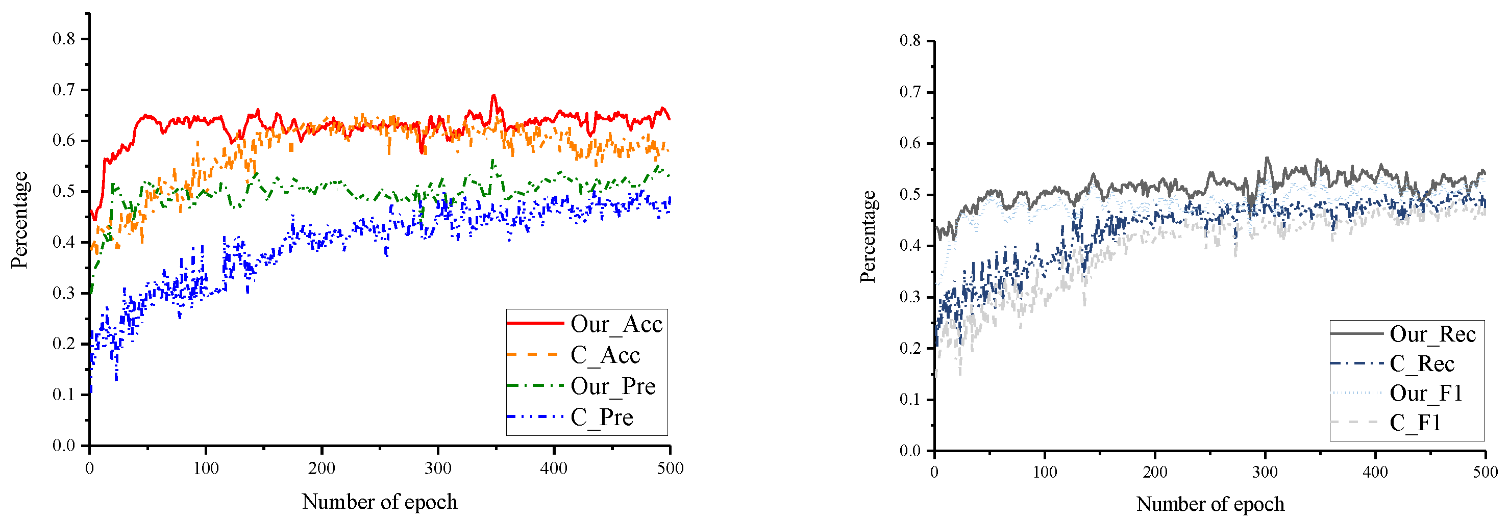
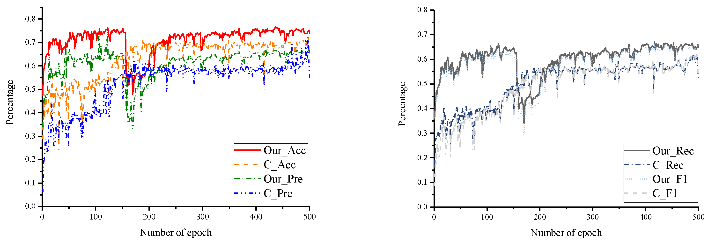
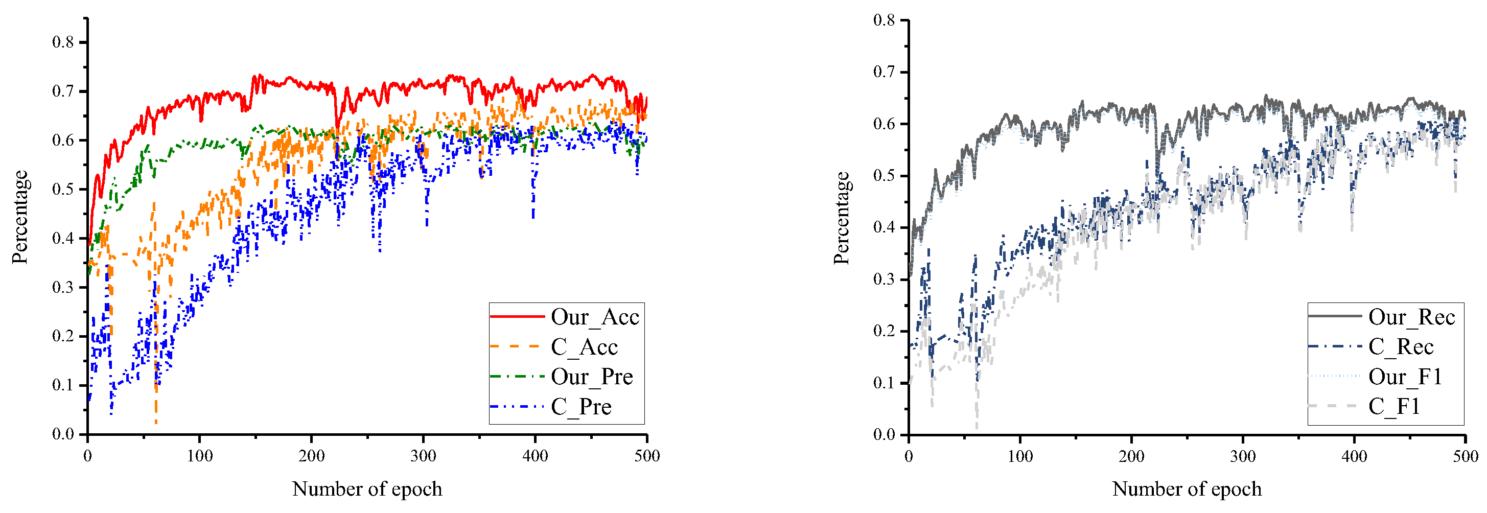
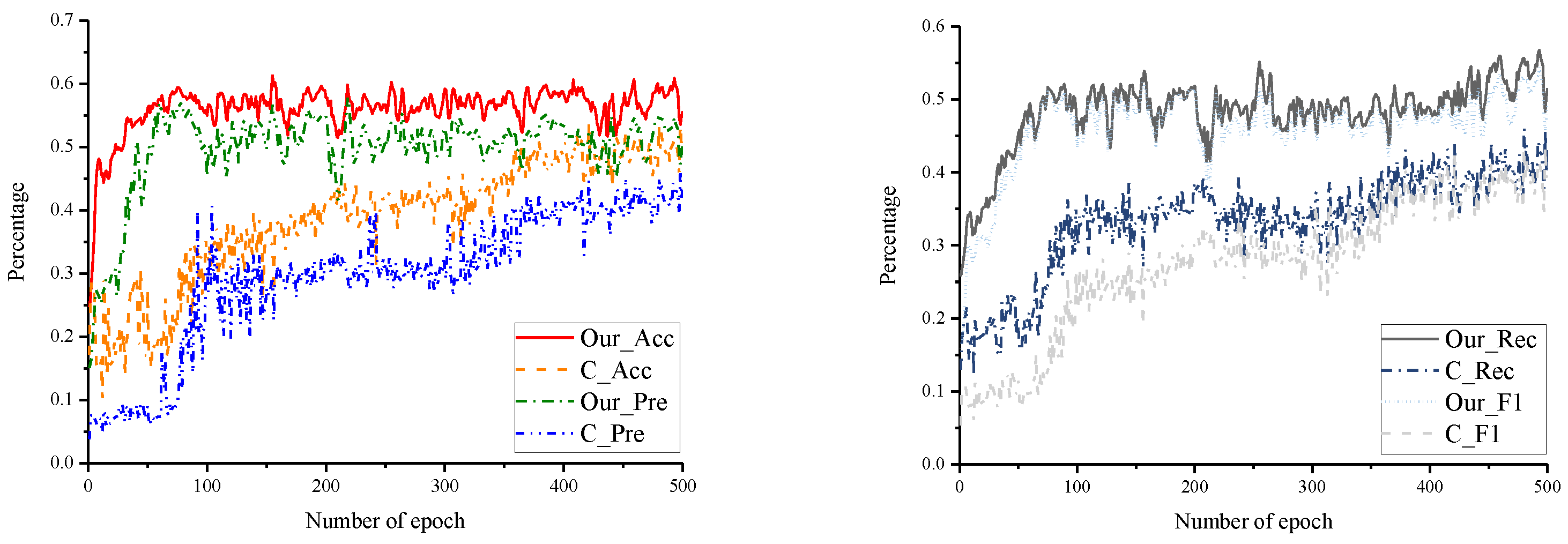
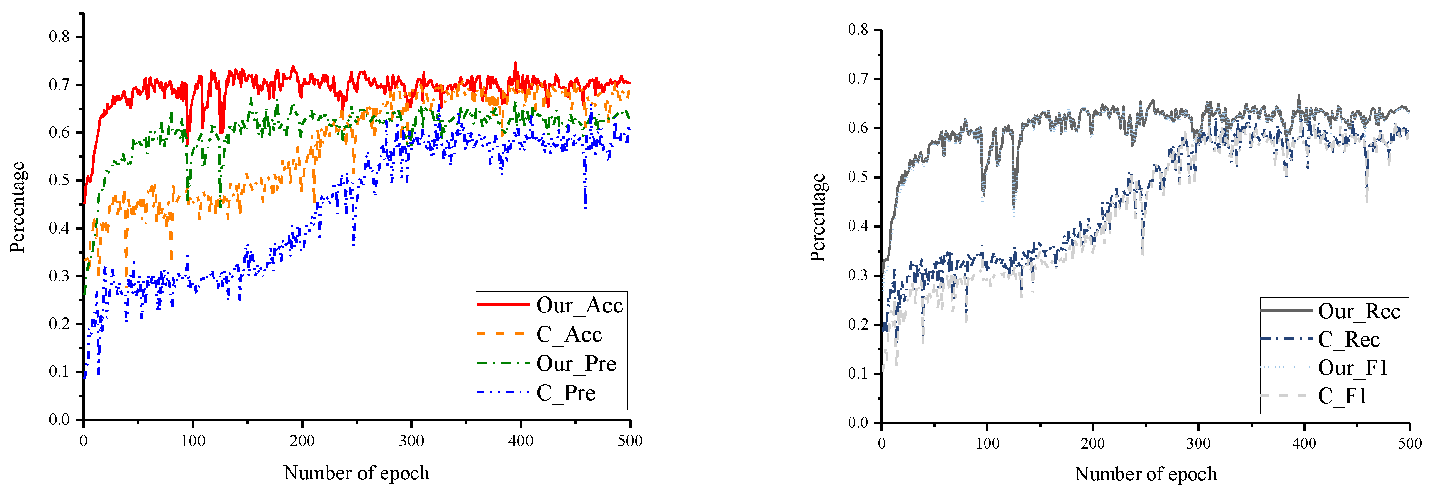
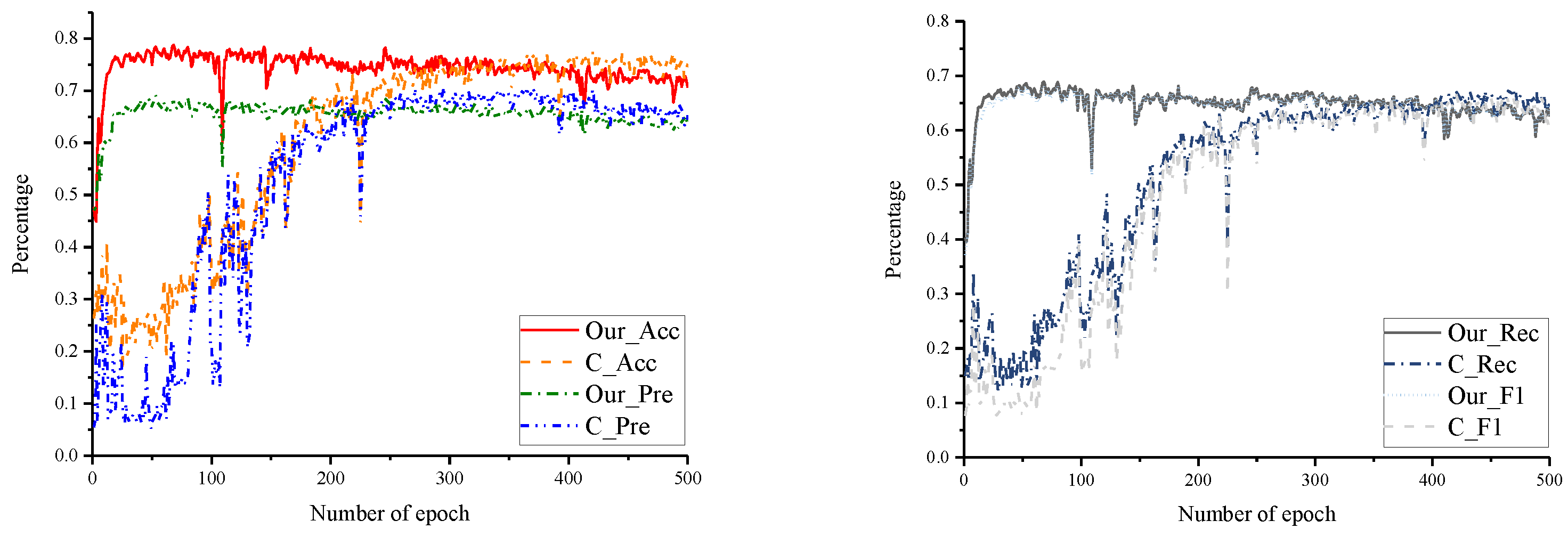
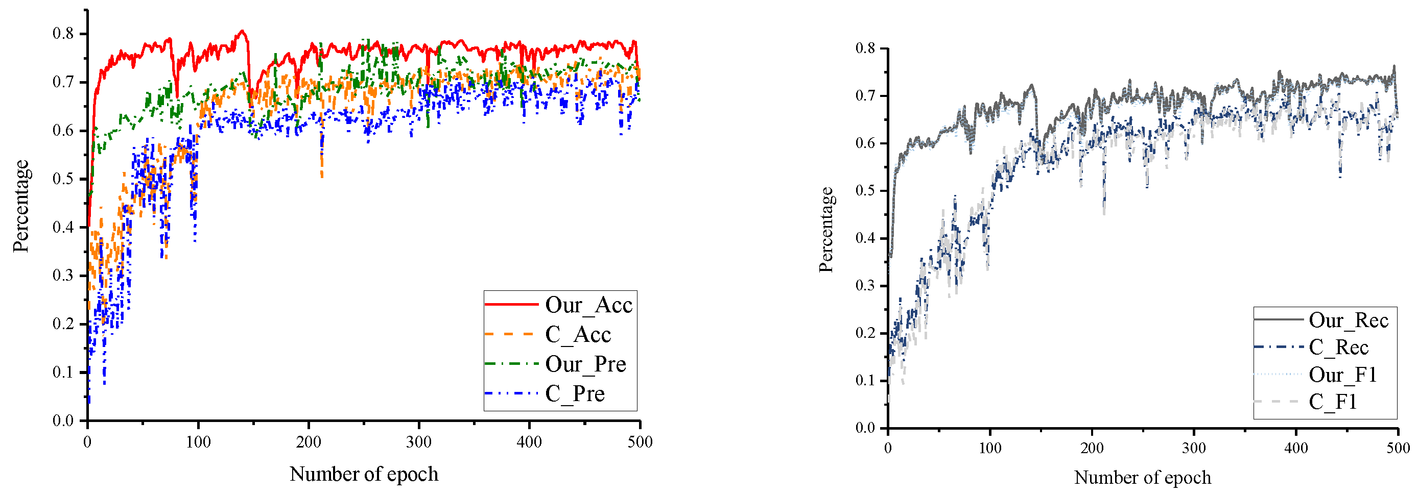
Firstly, the data from the source domain were used as the training set to pre-train the network model. We used accuracy as a metric to save the best pre-trained model. Additionally, the accuracy of each pre-trained model selected ranged from approximately 88% to 98%. Then, we took the network parameters of each layer and loaded them into the new network model. Finally, we fine-tuned the whole network with some data from the target domain. We need to note that it is better to choose a smaller learning rate when fine-tuning the network. Since the trained network model weights are already smoothed, we do not want to distort them too quickly. Our comparison experiment used data from the source domain and part of the target domain as the training set, and tested the remaining data in the target domain, i.e., without fine-tuning. The basic parameters of experiments are shown in Table 4. Additionally, the settings of the training and test sets are shown in Table 5. All results are shown in Table 5 and in Figure 4, Figure 5, Figure 6, Figure 7, Figure 8, Figure 9, Figure 10, Figure 11, Figure 12, Figure 13, Figure 14 and Figure 15.
For each set of experiments, the results are shown in Figure 4, Figure 5, Figure 6, Figure 7, Figure 8, Figure 9, Figure 10, Figure 11, Figure 12, Figure 13, Figure 14 and Figure 15. The following analysis of the improvement of each indicator is based on the indicators that work best in our method and in the comparison method.
As shown in Figure 4, HH101 is the source domain and HH105 is the target domain. Our method achieved better activity recognition at the 50th iteration and tended to stabilize thereafter, peaking at the 348th iteration; the comparison method stabilized at around the 200th iteration, peaking at the 259th. However, our method was able to approach the peak of the comparison method at an early stage and remained stable. Additionally, our method improved 3.07% in accuracy, 9.48% in precision, 8.61% in recall and 9.91% in F1-score over that of the comparison method.
As shown in Figure 5, HH101 is the source domain and HH109 is the target domain. Our method achieved better activity recognition at the 100th iteration, peaking at the 434th iteration; the comparison method achieved better activity recognition at the 250th iteration, peaking at the 256th. However, on every iteration, our method outperformed the comparison method. Our method improved 4.08% in accuracy, 10.94% in recall and 10.23% in F1-score over those of the comparison method. In addition, the precision was on a par with that of the comparison method.
As shown in Figure 6, HH101 is the source domain and HH110 is the target domain. Our method led the comparison method from the beginning to the end and remained stable throughout, peaking at the 119th iteration; the comparison method peaked at the 378th iteration. Our method improved 5.43% in accuracy and 1.58% in F1-score over those of the comparison method. Additionally, precision and recall were on par with that of the comparison method.
As shown in Figure 7, HH105 is the source domain and HH101 is the target domain. Our method achieved better recognition at the 50–150th iteration and remained stable after the 250th iteration; the comparison method remained stable only after the 250th iteration, but the accuracy results were consistently lower than those of our method. Our method improved 4.26% in accuracy, 5.35% in recall and 3.46% in F1-score over those of the comparison method. In addition, the precision was on a par with that of the comparison method.
As shown in Figure 8 and Figure 9, HH105 is the source domain and HH109/HH110 is the target domain. Our method achieved a high level of accuracy after a smaller number of iterations and consistently led the comparison methods with a high level of accuracy. In Figure 8, our method improved 3.96% in accuracy, 4.30% in recall and 3.34% in F1-score over those of the comparison method. In addition, the precision was on a par with that of the comparison method. In Figure 9, our method improved 7.53% in accuracy, 12.13% in precision, 8.93% in recall and 9.98% in F1-score over those of the comparison method. In addition, the performance of the fine-tuned model was very stable, which demonstrates the effectiveness of our migration method on LSTMs.
As shown in Figure 10, Figure 11 and Figure 12, our method achieved a high level of accuracy in less than 50 iterations and remained stable, whereas the comparison method took 200–300 iterations to reach stability. Additionally, our method generally improved accuracy by 3.07–6.27% over that of the comparison method. In Figure 10, our method improved the precision by 6.12% and the F1-score by 6.05%; in Figure 12, our method improved the precision by 7.63%; the rest of the indicators were at the same level as those of the comparison method.
As shown in Figure 13, at the end of the iteration, our proposed method was close to the recognition results of the comparison method. However, our method achieved more than 75% accuracy almost at the beginning of the phase, and the comparison method did not reach a similar level until the 300th iteration. This demonstrates that fine-tuning methods on LSTMs can learn the knowledge of the target domain extremely quickly and make corrections to the network parameters, achieving strong migration effects in a shorter period of time.
As shown in Figure 14, our method showed considerable superiority, improving accuracy by 10.16%, recall by 9.17% and F1-score by 8.8% over those of the comparison method. In addition, the precision remained on par with that of the comparison method. Additionally, as seen in Figure 15, our method’s metrics were also consistently higher than those of the comparison method, improving accuracy by 4.87%, recall by 3.39% and F1-score by 1.5% over those of the comparison method.
By analyzing the above graphs and charts, we can observe that the accuracy was improved by 0.7–10.6% and most experiments improved by 3–5%. The precision was improved by up to 12.13%, the recall was improved by up to 10.94% and the F1-score was improved by up to 10.23% compared with those of the direct training. Additionally, the learning efficiency of the fine-tuned network was fast, and most results were optimal in about 50–100 epochs. This is because the fine-tuning incorporates the parameters of the pre-trained model. Based on this, the classification weights of the network can be corrected with a small amount of training data to achieve better classification results. This shows that our proposed fine-tuning method demonstrates excellent transfer effects on the domain of daily activity recognition and exhibits strong stability and generalization. Furthermore, the training time of the fine-tuning method is less than one-third of the time required for training from scratch, which greatly saves training time.
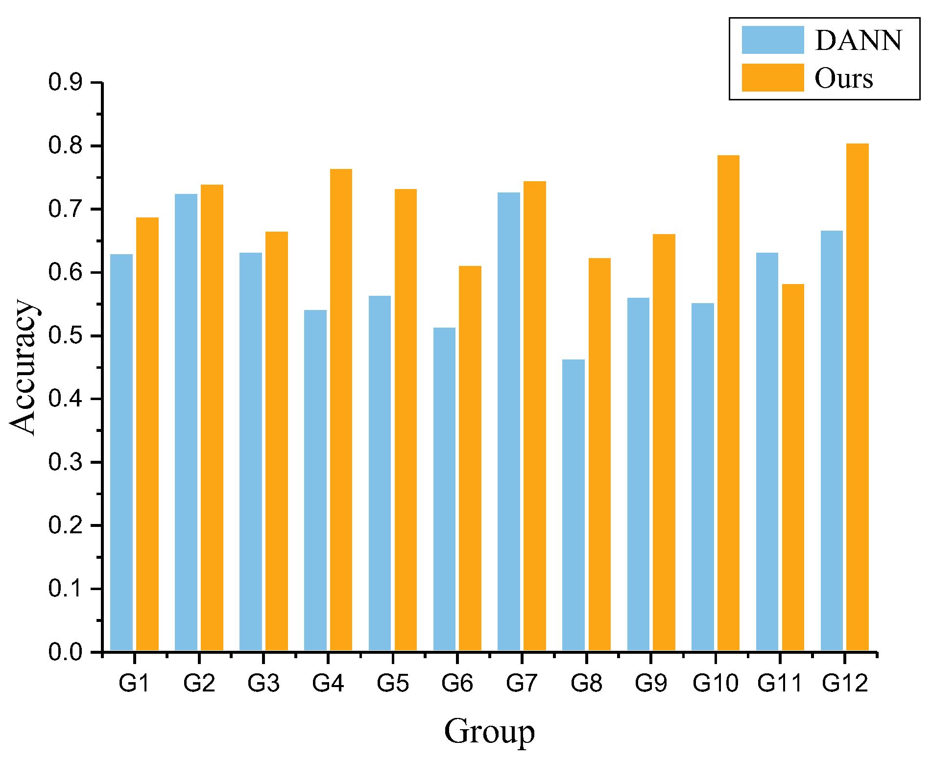
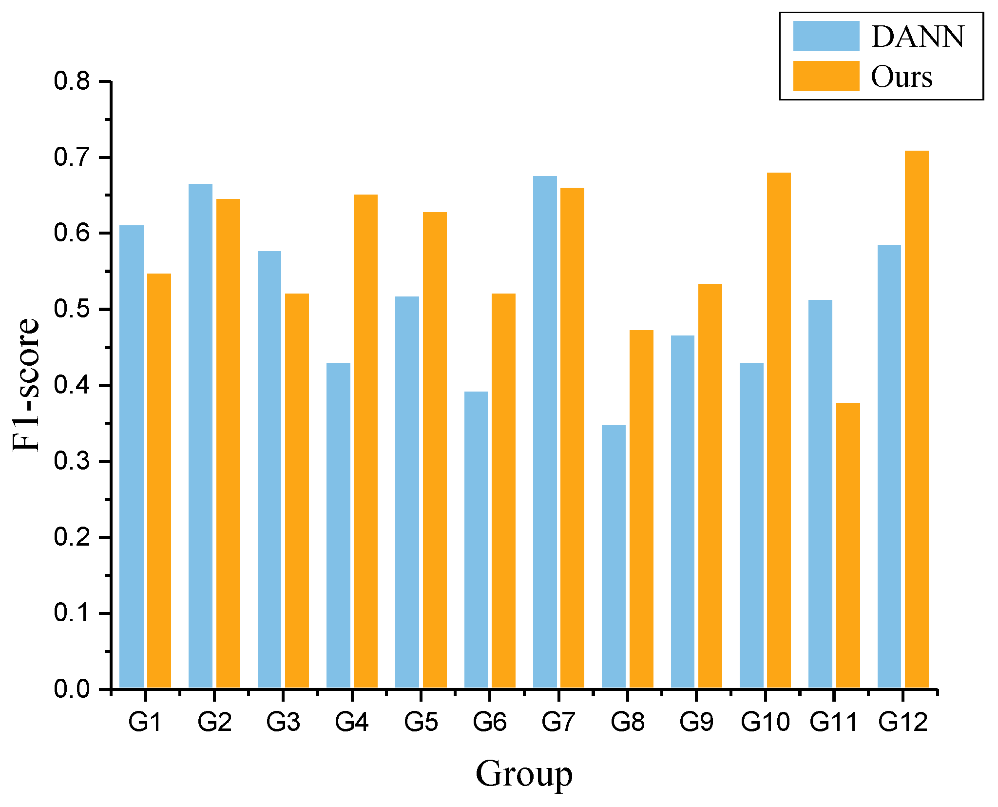
In addition, we have compared the existing deep migration method for daily activity recognition. The method mainly uses the Domain Adaptive Neural Network (DANN) for model migration. Additionally, the experimental setups are shown in Table 6. As can be seen from Table 6 and Figure 16, Figure 17 and Figure 18, our method outperformed the DANN method on all datasets, except for Group 11. Accuracy improved by more than 10% within most groups, and even by 23% in group 10. Precision and F1-score also improved on most of the datasets.

5. Conclusions and Future Work

In this paper, we explore a suitable deep neural network LSTM for the smart home domain. Additionally, we conduct extensive experiments on the CASAS dataset. We fine-tuned for small datasets, effectively improving recognition accuracy even better than direct training. At the same time, the fine-tuning greatly saves training time. It can be seen that in the initial epoch, the training accuracy rises quickly and reaches the best soon. We note that this is the first time that fine-tuning has made results in the smart home domain. This is exciting and means that the deep network has good transferability in the field of daily activity recognition in smart homes, instead of its superior performance in the image domain.
In the future, we hope we can build a library of fine-tuned network models based on smart homes together with you. Additionally, we will conduct further research on network migration at different levels. Additionally, we intend to add adaptive layers at some important levels to make the data distribution more similar and enhance the effect of fine-tuning.

Author Contributions

Conceptualization, Y.L. and Y.Y.; methodology, Y.L. and Y.Y.; validation, K.T.; data curation, K.T. and Y.L.; writing–review and editing, Y.L. and Y.Y. All authors have read and agreed to the published version of the manuscript.

Funding

This research received no external funding.

Institutional Review Board Statement

Not applicable.

Informed Consent Statement

Not applicable.

Data Availability Statement

The dataset is available at https://casas.wsu.edu/datasets/ (accessed on 25 April 2023).

Conflicts of Interest

The authors declare no conflict of interest.

References

  1. Liu, Y.; Xie, R.; Gong, S. Interaction-Feedback Network for Multi-Task Daily Activity Forecasting. Expert Syst. Appl. 2023, 218, 119602. [Google Scholar] [CrossRef]
  2. Kasteren, V.; Englebienne, G.; Krose, B.J.A. Recognizing activities in multiple contexts using transfer learning. In Proceedings of the AAAI Symposium, Arlington, VA, USA, 7–9 November 2008; pp. 142–149. [Google Scholar]
  3. Pan, S.J.; Qiang, Y. A survey on transfer learning. IEEE Trans. Knowl. Data Eng. 2010, 22, 1345–1359. [Google Scholar] [CrossRef]
  4. Cook, D.; Feuz, K.D.; Krishnan, N.C. Transfer learning for activity recognition: A survey. Knowl. Inf. Syst. 2013, 36, 537–556. [Google Scholar] [CrossRef] [PubMed]
  5. Yu, Y.; Hao, Z.; Li, G.; Liu, Y.; Yang, R.; Liu, H. Optimal search mapping among sensors in heterogeneous smart homes. Math. Biosci. Eng. 2023, 20, 1960–1980. [Google Scholar] [CrossRef]
  6. Fawaz, H.I.; Forestier, G.; Weber, J.; Idoumghar, L.; Muller, P.-A. Transfer learning for time series classification. In Proceedings of the IEEE International Conference on Big Data, Seattle, WA, USA, 10–13 December 2018. [Google Scholar]
  7. Chen, Y.; Keogh, E.; Hu, B.; Yeh, C.C.M.; Zhu, Y.; Gharghabi, S.; Ratanamahatana, C.A.; Keogh, E. The UCR Time Series Classification Archive. 2015. Available online: https://www.cs.ucr.edu/~eamonn/time_series_data_2018 (accessed on 15 October 2018).
  8. Cook, D.J.; Crandall, A.S.; Thomas, B.L.; Krishnan, N.C. CASAS: A smart home in a box. Computer 2013, 46, 62–69. [Google Scholar] [CrossRef]
  9. Ye, J.; Dobson, S.; Zambonelli, F. XLearn: Learning activity labels across heterogeneous datasets. ACM Trans. Intell. Syst. Technol. 2020, 11, 28. [Google Scholar] [CrossRef]
  10. Feuz, K.D.; Cook, D.J. Transfer learning across feature-rich heterogeneous feature spaces via feature-space remapping (FSR). Acm Trans. Intell. Syst. Technol. 2015, 6, 1–27. [Google Scholar] [CrossRef]
  11. Azkune, G.; Almeida, A.; Agirre, E. Cross-environment activity recognition using word embeddings for sensor and activity representation. Neurocomputing 2020, 418, 280–290. [Google Scholar] [CrossRef]
  12. Chiang, Y.T.; Hsu, Y.J. Knowledge transfer in activity recognition using sensor profile. In Proceedings of the International Conference on Ubiquitous Intelligence and Computing and International Conference on Autonomic and Trusted Computing, Washington, DC, USA, 4–7 September 2012; pp. 180–187. [Google Scholar]
  13. Hu, D.H.; Yang, Q. Transfer learning for activity recognition via sensor mapping. In Proceedings of the Twenty-Second International Joint Conference on Artificial Intelligence, Barcelona, Spain, 16–22 July 2011; pp. 1962–1967. [Google Scholar]
  14. Rashidi, P.; Cook, D.J. Activity Recognition Based on Home to Home Transfer Learning; AAAI Press: New Orleans, LA, USA, 2010. [Google Scholar]
  15. Hu, D.H.; Zheng, V.W.; Yang, Q. Cross-domain activity recognition via transfer learning. Pervasive Mob. Comput. 2011, 7, 344–358. [Google Scholar] [CrossRef]
  16. Yosinski, J.; Clune, J.; Bengio, Y. How transferable are features in deep neural networks? Adv. Neural Inf. Process. Syst. 2014, 7, 3320–3328. [Google Scholar]
  17. Krizhevsky, A.; Sutskever, I.; Hinton, G.E. Imagenet classification with deep convolutional neural networks. Adv. Neural Inf. Process. Syst. 2012, 25, 1097–1105. [Google Scholar] [CrossRef]
  18. Tzeng, E.; Hoffman, J.; Zhang, N.; Saenko, K.; Darrell, T. Deep domain confusion: Maximizing for domain invariance. arXiv 2014, arXiv:1412.3474. [Google Scholar]
  19. Borgwardt, K.M.; Gretton, A.; Rasch, M.J.; Kriegel, H.-P.; Schölkopf, B.; Smola, A.J. Integrating structured biological data by kernel maximum mean discrepancy. Bioinformatics 2006, 22, e49–e57. [Google Scholar] [CrossRef] [PubMed]
  20. Long, M.; Cao, Y.; Wang, J.; Jordan, M. Learning transferable features with deep adaptation networks. In Proceedings of the International Conference on Machine Learning, Lille, France, 6–11 July 2015; pp. 97–105. [Google Scholar]
  21. Gretton, A.; Sejdinovic, D.; Strathmann, H.; Balakrishnan, S.; Pontil, M.; Fukumizu, K.; Sriperumbudur, B.K. Optimal kernel choice for largescale two-sample tests. Adv. Neural Inf. Process. Syst. 2012, 25, 1205–1213. [Google Scholar]
  22. Zhuo, J.; Wang, S.; Zhang, W.; Huang, Q. Deep unsupervised convolutional domain adaptation. In Proceedings of the 2017 ACM on Multimedia Conference, Mountain View, CA, USA, 23–27 October 2017; pp. 261–269. [Google Scholar]
  23. Long, M.; Wang, J.; Cao, Y.; Sun, J.; Yu, P.S. Deep learning of transferable representation for scalable domain adaptation. IEEE Trans. Knowl. Data Eng. 2016, 28, 2027–2040. [Google Scholar] [CrossRef]
  24. Sun, B.; Saenko, K. Deep coral: Correlation Alignment for Deep Domain Adaptation. In Proceedings of the European Conference on Computer Vision, Amsterdam, The Netherlands, 11–14 October 2016; pp. 443–450. [Google Scholar]
  25. Wei, P.; Ke, Y.; Goh, C.K. Deep nonlinear feature coding for unsupervised domain adaptation. In Proceedings of the International Joint Conference on Artificial Intelligence, New York, NY, USA, 9–15 July 2016; pp. 2189–2195. [Google Scholar]
  26. Zhuang, F.; Cheng, X.; Luo, P.; Pan, S.J.; He, Q. Supervised Representation Learning: Transfer Learning with Deep Autoencoders. In Proceedings of the International Joint Conference on Artificial Intelligence, Buenos Aires, Argentina, 25–31 July 2015; pp. 4119–4125. [Google Scholar]
  27. Luo, Z.; Zou, Y.; Hoffman, J.; Fei-Fei, L.F. Label efficient learning of transferable representations acrosss domains and tasks. Adv. Neural Inf. Process. Syst. 2017, 30, 164–176. [Google Scholar]
  28. Petitjean, F.; Ganarski, P. Summarizing a set of time series by averaging: From steiner sequence to compact multiple alignment. Theor. Comput. Sci. 2012, 414, 76–91. [Google Scholar] [CrossRef]
  29. Sun, Y.G.; Kim, S.H.; Lee, S.; Seon, J.; Lee, S.; Kim, C.G.; Kim, J.Y. Performance of End-to-end Model Based on Convolutional LSTM for Human Activity Recognition. J. Web Eng. 2022, 21, 1671–1690. [Google Scholar] [CrossRef]
  30. Singh, D.; Merdivan, E.; Hanke, S.; Geist, M.; Holzinger, A. Convolutional and Recurrent Neural Networks for Activity Recognition in Smart Environment. In Proceedings of the Banff-International-Research-Station (BIRS) Workshop, Banff, AB, Canada, 24–26 July 2015; pp. 194–205. [Google Scholar]
  31. Liciotti, D.; Bernardini, M.; Romeo, L.; Frontoni, E. A sequential deep learning application for recognising human activities in smart homes. Neurocomputing 2020, 396, 501–513. [Google Scholar] [CrossRef]
  32. Thapa, K.; Mi, Z.M.A.; Sung-Hyun, Y. Adapted Long Short-Term Memory (LSTM) for Concurrent Human Activity Recognition. Cmc Comput. Mater. Contin. 2021, 69, 1653–1670. [Google Scholar] [CrossRef]
  33. Forbes, G.; Massie, S.; Craw, S.; Fraser, L.; Hamilton, G. Representing Temporal Dependencies in Smart Home Activity Recognition for Health Monitoring. In Proceedings of the International Joint Conference on Neural Networks, Glasgow, UK, 19–24 July 2020; pp. 1–8. [Google Scholar]
  34. Mikolov, T.; Chen, K.; Corrado, G.; Dean, J. Efficient estimation of word representations in vector space. arXiv 2013, arXiv:1301.3781. [Google Scholar]
  35. Anguita, D.; Ghio, A.; Oneto, L.; Parra, X.; Reyes-Ortiz, J.L. A public domain dataset for human activity recognition using smartphones. In Proceedings of the European Symposium on Artificial Neural Networks, Computational Intelligence and Machine Learning, Bruges, Belgium, 24–26 April 2013; pp. 437–442. [Google Scholar]
  36. Bengio, Y.; Glorot, X. Understanding the difficulty of training deep feed forward neural networks. Int. Conf. Artif. Intell. Stat. 2010, 9, 249–256. [Google Scholar]
Figure 1. Method flow.
Applsci 13 05706 g001
Figure 2. Data pre-processing method flow.
Applsci 13 05706 g002
Figure 3. LSTM network.
Applsci 13 05706 g003
Figure 4. Results of our method and comparison experiments for accuracy, precision, recall and F1-score at each epoch, based on the source domain as HH101, target domain as HH105.
Applsci 13 05706 g004
Figure 5. Results of our method and comparison experiments for accuracy, precision, recall and F1-score at each epoch, based on the source domain as HH101, target domain as HH109.
Applsci 13 05706 g005
Figure 6. Results of our method and comparison experiments for accuracy, precision, recall and F1-score at each epoch, based on the source domain as HH101, target domain as HH110.
Applsci 13 05706 g006
Figure 7. Results of our method and comparison experiments for accuracy, precision, recall and F1-score at each epoch, based on the source domain as HH105, target domain as HH101.
Applsci 13 05706 g007
Figure 8. Results of our method and comparison experiments for accuracy, precision, recall and F1-score at each epoch, based on the source domain as HH105, target domain as HH109.
Applsci 13 05706 g008
Figure 9. Results of our method and comparison experiments for accuracy, precision, recall and F1-score at each epoch, based on the source domain as HH105, target domain as HH110.
Applsci 13 05706 g009
Figure 10. Results of our method and comparison experiments for accuracy, precision, recall and F1-score at each epoch, based on the source domain as HH109, target domain as HH101.
Applsci 13 05706 g010
Figure 11. Results of our method and comparison experiments for accuracy, precision, recall and F1-score at each epoch, based on the source domain as HH109, target domain as HH105.
Applsci 13 05706 g011
Figure 12. Results of our method and comparison experiments for accuracy, precision, recall and F1-score at each epoch, based on the source domain as HH109, target domain as HH110.
Applsci 13 05706 g012
Figure 13. Results of our method and comparison experiments for accuracy, precision, recall and F1-score at each epoch, based on the source domain as HH110, target domain as HH101.
Applsci 13 05706 g013
Figure 14. Results of our method and comparison experiments for accuracy, precision, recall and F1-score at each epoch, based on the source domain as HH110, target domain as HH105.
Applsci 13 05706 g014
Figure 15. Results of our method and comparison experiments for accuracy, precision, recall and F1-score at each epoch, based on the source domain as HH110, target domain as HH109.
Applsci 13 05706 g015
Figure 16. Accuracy of our method and that of DANN, based on Group 1 to Group 12.
Applsci 13 05706 g016
Figure 17. Precision of our method and that of DANN, based on Group 1 to Group 12.
Applsci 13 05706 g017
Figure 18. F1-score of our method and that of DANN, based on Group 1 to Group 12.
Applsci 13 05706 g018
Table 1. An example of a “Sleep_Out_Of_Bed” activity in source domain.
dtsn svac
20 July 201215/04/47. 939431M008ONSleep_Out_Of_Bed
20 July 201215/04/49. 047095LS00838
20 July 201215/04/49. 11856M008OFF
20 July 201215/09/05. 634721LS01227
20 July 201215/09/49. 513611LS00926
20 July 201215/10/37. 143058LS01435
20 July 201215/10/44. 79274LS00112
20 July 201215/12/01. 593479LS0036
20 July 201215/12/44. 773366LS01615
20 July 201215/12/47. 7472LS00414
20 July 201215/12/53. 867533LS01327
20 July 201215/13/29. 44345LS01120
20 July 201215/19/05. 563968LS01226
20 July 201215/19/49. 404442LS00923
20 July 201215/20/37. 05254LS01431
20 July 201215/20/44. 684768LS00110
20 July 201215/21/51. 214887LS00834
20 July 201215/21/51. 241965M008ON
20 July 201215/21/52. 330604M008OFF
Table 2. Example of a unified sensor space.
Source DomainTarget DomainLocationTypeRename
LS009, LS012, LS014LS013, LS014, LS015BedroomLightBedroom_Light
M002, M003M008, M010BedroomMotionBedroom_Motion
D003D003ToiletDoorToilet_Door
Table 3. The distribution of functional areas in the selected smart homes.
Smart HomeKitchenDiningParlorPorchToiletBedroomPorch_Toilet
HH1011111111
HH1051111111
HH1091111111
HH1101111111
Table 4. Parameters of the LSTM network for our method and comparison method.
WindowLearning RateDropoutOptimizerBatch SizeEpochLoss Function
Ours100Model: 0.001 Fine-tuning: 0.000010.5Adam64500Cross-entropy
Comparison1000.0010.5Adam64500Cross-entropy
Table 5. Experimental setup and results of our method and the comparison method.
ExperimentTraining SetTest SetAccuracy
Group
1
Ours_101to1051 × HH101 + Fine-tuning(0.2 × HH105)0.8 × HH1050.6899
Comparison_101to1051 × HH101 + 0.2 × HH1050.8 × HH1050.6592
Group
2
Ours_101to1091 × HH101 + Fine-tuning(0.2 × HH109)0.8 × HH1090.7413
Comparison_101to1091 × HH101 + 0.2 × HH1090.8 × HH1090.7004
Group
3
Ours_101to1101 × HH101 + Fine-tuning(0.2 × HH110)0.8 × HH1100.6673
Comparison_101to1101 × HH101 + 0.2 × HH1100.8 × HH1100.6129
Group
4
Ours_105to1011 × HH105 + Fine-tuning(0.2 × HH101)0.8 × HH1010.7664
Comparison_105to1011 × HH105 + 0.2 × HH1010.8 × HH1010.7238
Group
5
Ours_105to1091 × HH105 + Fine-tuning(0.2 × HH109)0.8 × HH1090.7339
Comparison_105to1091 × HH105 + 0.2 × HH1090.8 × HH1090.6943
Group
6
Ours_105to1101 × HH105 + Fine-tuning(0.2 × HH110)0.8 × HH1100.6129
Comparison_105to1101 × HH105 + 0.2 × HH1100.8 × HH1100.5376
Group
7
Ours_109to1011 × HH109 + Fine-tuning(0.2 × HH101)0.8 × HH1010.7468
Comparison_109to1011 × HH109 + 0.2 × HH1010.8 × HH1010.7131
Group
8
Ours_109to1051 × HH109 + Fine-tuning(0.2 × HH105)0.8 × HH1050.6256
Comparison_109to1051 × HH109 + 0.2 × HH1050.8 × HH1050.5949
Group
9
Ours_109to1101 × HH109 + Fine-tuning(0.2 × HH110)0.8 × HH1100.6631
Comparison_109to1101 × HH109 + 0.2 × HH1100.8 × HH1100.6004
Group
10
Ours_110to1011 × HH110 + Fine-tuning(0.2 × HH101)0.8 × HH1010.7877
Comparison_110to1011 × HH110 + 0.2 × HH1010.8 × HH1010.7806
Group
11
Ours_110to1051 × HH110 + Fine-tuning(0.2 × HH105)0.8 × HH1050.5837
Comparison_110to1051 × HH110 + 0.2 × HH1050.8 × HH1050.4776
Group
12
Ours_110to1091 × HH110 + Fine-tuning(0.2 × HH109)0.8 × HH1090.8069
Comparison_110to1091 × HH110 + 0.2 × HH1090.8 × HH1090.7586
Table 6. Experimental setup and results of our method and the DANN method.
GroupExperimentTraining SetTest SetAccuracy
1Ours_101to1051 × HH101 + Fine-tuning(0.2 × HH105)0.8 × HH1050.6899
DANN_101to1051 × HH101 + 0.2 × HH1050.8 × HH1050.6312
2Ours_101to1091 × HH101 + Fine-tuning(0.2 × HH109)0.8 × HH1090.7413
DANN_101to1091 × HH101 + 0.2 × HH1090.8 × HH1090.7265
3Ours_101to1101 × HH101 + Fine-tuning(0.2 × HH110)0.8 × HH1100.6673
DANN_101to1101 × HH101 + 0.2 × HH1100.8 × HH1100.6343
4Ours_105to1011 × HH105 + Fine-tuning(0.2 × HH101)0.8 × HH1010.7664
DANN_105to1011 × HH105 + 0.2 × HH1010.8 × HH1010.5437
5Ours_105to1091 × HH105 + Fine-tuning(0.2 × HH109)0.8 × HH1090.7339
DANN_105to1091 × HH105 + 0.2 × HH1090.8 × HH1090.5656
6Ours_105to1101 × HH105 + Fine-tuning(0.2 × HH110)0.8 × HH1100.6129
DANN_105to1101 × HH105 + 0.2 × HH1100.8 × HH1100.5156
7Ours_109to1011 × HH109 + Fine-tuning(0.2 × HH101)0.8 × HH1010.7468
DANN_109to1011 × HH109 + 0.2 × HH1010.8 × HH1010.7296
8Ours_109to1051 × HH109 + Fine-tuning(0.2 × HH105)0.8 × HH1050.6256
DANN_109to1051 × HH109 + 0.2 × HH1050.8 × HH1050.4656
9Ours_109to1101 × HH109 + Fine-tuning(0.2 × HH110)0.8 × HH1100.6631
DANN_109to1101 × HH109 + 0.2 × HH1100.8 × HH1100.5625
10Ours_110to1011 × HH110 + Fine-tuning(0.2 × HH101)0.8 × HH1010. 7877
DANN_110to1011 × HH110 + 0.2 × HH1010.8 × HH1010.5546
11Ours_110to1051 × HH110 + Fine-tuning(0.2 × HH105)0.8 × HH1050. 5837
DANN_110to1051 × HH110 + 0.2 × HH1050.8 × HH1050.6343
12Ours_110to1091 × HH110 + Fine-tuning(0.2 × HH109)0.8 × HH1090.8069
DANN_110to1091 × HH110 + 0.2 × HH1090.8 × HH1090.6687
Disclaimer/Publisher’s Note: The statements, opinions and data contained in all publications are solely those of the individual author(s) and contributor(s) and not of MDPI and/or the editor(s). MDPI and/or the editor(s) disclaim responsibility for any injury to people or property resulting from any ideas, methods, instructions or products referred to in the content.