Abstract
In this paper, a comprehensive probabilistic framework is proposed and adopted to perform seismic reliability and risk analysis of existing link slab (LS) bridges, representing a widely diffused structural typology within the infrastructural networks of many countries worldwide. Unlike classic risk analysis methods, innovative fragility functions are used in this work to retrieve more specific and detailed information on the possible failure modes, without limiting the analysis to the global failure conditions but also considering several intermediate damage scenarios (including one or more damage mechanisms), and providing insights on the numerosity of elements involved within a given damage scenario. Reliability analyses are performed on a set of LS bridges with different geometries (total lengths and pier heights) designed according to the Italian codes enforced in the 1970s. Accurate numerical models are developed in OpenSees and Multiple-Stripe nonlinear time–history analyses are carried out to build proper demand models, from which fragility functions are determined according to two limit states: damage onset and near-collapse. Mean annual rates of exceeding are thus estimated through the convolution between the hazard and the fragility. The results shed light on the main failure mechanisms characterizing this bridge typology, highlighting how different levels of risk (hence safety margins) can be associated with failure scenarios that differ in terms of elements/mechanisms involved and damage extension. Such a higher level of detail in the risk analysis may be useful to better quantify post-earthquake consequences (e.g., costs and losses) and define more tailored retrofit interventions. A comparison of the reliability levels associated with bridges of the same class with different geometries is finally presented.
1. Introduction
Bridges play a critical role within transportation and infrastructure networks. Their disruption can have a significant socioeconomic impact and their failure can jeopardize people’s lives [1]. Over the last few decades, we have witnessed a significant growth of scientific literature focusing on vulnerability and risk assessment of bridges under diverse sources of danger. For instance, numerous studies have been focused on seismic-related problems (hazard, design, assessment, retrofit) [2,3,4,5,6]; other works have been dedicated to flood and scour [7,8,9,10], which are also serious phenomena undermining bridge stability and integrity. Some recent studies have been dedicated to special subjects, such as the reliability of existing prestressed bridges [11,12], structural health monitoring strategies [13,14], bridge inspection data analysis [15], and safety assessment under traffic loads [16].
Within such a wide context concerning bridges, the current paper focuses on the seismic reliability analysis of a widespread typology of bridges characterizing a broad percentage of the existing infrastructural networks worldwide. The systems at hand are represented by the class of multi-span simply supported reinforced concrete (RC) Link Slab (LS) bridges, based on a technology that has been widely employed over the past 50 years to realize structural joints in bridge superstructures [17,18,19,20,21]. It is known that expansion joints are traditionally provided and designed to accommodate deformations induced by temperature gradients in order to avoid structural problems, and they usually are effective in this aim, though some issues may arise when water drains through them, penetrating the substructures (piers and abutments), and thus contributing to and accelerating the degradation process of bearing devices and substructure themselves (Figure 1a). These joints are moreover prone to ruin because of the gradual accumulation of materials within them (Figure 1b).

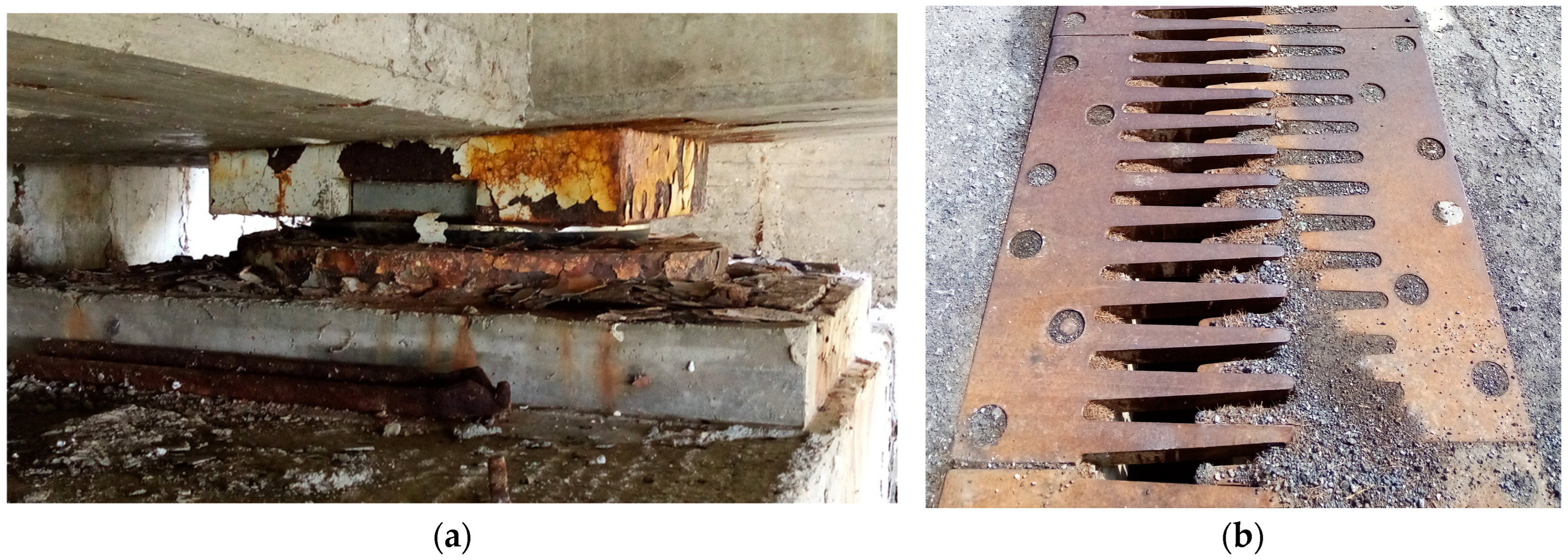
Figure 1.
(a) Typical consequences of the expansion joints permeability: degradation and corrosion of a cylindrical hinge bearing device. (b) Debris and materials accumulation within an expansion joint compromising its functionality.
Continuous bridges can represent a solution to the aforementioned issues, but at the expense of generally higher complexity in the design process. A widely used alternative strategy to realize jointless bridges without renouncing the advantages of simply supported static schemes is exploiting a link slab solution. This allows the connection of the decks belonging to adjacent simply supported spans without resorting to specific expansion joint devices. In general, this solution is employed to realize one or more kinematic chains, composed of a given amount of jointless spans and a limited number of traditional expansion joints located at the end of these chains (and usually in correspondence with one of the two abutments), with the advantage of increasing the smoothness (consequently the safety) of driving, eliminating problems relating to atmospheric agents penetration on substructures.
The large presence of existing bridges adopting this technology, designed and built before the entrance in force of proper and detailed seismic codes, is the main reason behind this study. Indeed, a thorough analysis of the seismic reliability offered by existing link slab-reinforced concrete bridges is, to date, missing in the scientific literature.
A comprehensive probabilistic framework is thus proposed and adopted in this study to perform seismic reliability and risk analysis of these systems. One of the key points of the framework is represented by a novel practical-oriented procedure for fragility analysis recently proposed by Minnucci et al. (2022) [22] with the aim of overcoming some limits of classical approaches and providing rapid and useful data to directly support the decision-making process.
Indeed, the common practice, according to the existing literature, is that of cataloging bridges within homogeneous fragility classes [23,24,25], performing fragility analysis focusing on either the overall performance of the bridge or based on a unique response parameter [26,27,28], where often an “in-series” system assumption is invoked for the evaluation of the global failure [29,30,31,32]. Some effort was made by a few authors to address the problem of multiple critical components in seismic assessment of bridges [33,34,35,36,37].
However, the main difference of the strategy adopted here with respect to the common approaches currently available relies on the capability of the novel fragility functions to retrieve more specific and detailed information on the possible failure modes, without limiting the analysis to the global failure conditions but also considering several intermediate damage scenarios (including one or more damage mechanisms), and providing insights on the numerosity of elements involved within a given damage scenario. For instance, while classic risk analysis approaches do not permit a wide spectrum of information on the expected damage conditions but only permit a global assessment (e.g., global attainment of a given limit state), the proposed methodology is capable of providing the probability of attainment of a given limit state by a specific structural component or by a group of two or more components.
A set of case studies is presented, consisting of LS RC bridges with different geometries, which have been preliminarily designed according to the codes that were enforced in Italy during the 1970s. These systems are modeled in OpenSees and Multiple-Stripe nonlinear time–history analyses are carried out to build proper demand models, from which various types of fragility functions are determined according to two limit states, the damage onset and near-collapse. Mean annual rates of exceeding are thus estimated for both limit states through the convolution between the hazard and the fragility. The results shed light on the main failure mechanisms characterizing this bridge typology, highlighting how different levels of risk (hence, safety margins) can be associated with failure scenarios that differ in terms of elements/mechanisms involved and damage extension.
A comparison in terms of annual rates of failure is made considering the different bridge geometries.
The paper structure is as follows. The methodology is presented in the former part of the manuscript in order to highlight the novelty and the strengths with respect to classic seismic vulnerability analysis. Case studies are then introduced providing details about the geometry, the simulated seismic design process, the numerical modeling strategy and the considered response parameters and related capacity thresholds. In Section 4, results are presented in terms of both fragility functions and mean annual rates of exceedance considering the damage onset and collapse limit state and quantitative insights concerning the reliability level achieved by these systems are provided. The paper ends with a conclusive section in which all the most relevant results are recapped.
2. Seismic Reliability Framework
In this work, a conditional probabilistic approach is used for the seismic performance assessment of bridges. This type of approach exploits an intensity measure (IM) to decompose the problem into separate tasks: hazard analysis and seismic demand analysis. In the following, these tasks are described in detail.
2.1. Seismic Scenario and Hazard
A typical scenario of medium-high seismicity regions in Italy is considered for the purposes of these applications.
As an intensity measure, IM, the maximum spectral acceleration component [38], IM = max{Sa,X(T), Sa,Y(T)}, is chosen for the following two reasons: (i) it allows accounting for the bidirectional features of the seismic input (both the horizontal, X and Y, seismic components are considered), (ii) unlike the Peak Ground Acceleration (PGA) [29], the spectral amplification related to the system dynamic properties can be accounted for through the definition of the vibration period, and an average period between transversal and longitudinal vibration modes is considered in this study. However, several alternative (scalar and vector-valued) IMs are also available but this aspect goes out of the scope of the present study.
A widely used and validated stochastic ground motion model [39,40] is adopted to characterize the underlying seismicity and provide a proper IM hazard curve (through the procedure detailed in the work [41]). Moreover, sets of synthetic ground motion samples are generated through the stochastic model in order to obtain a suitable database of earthquakes conditional to different IM levels, according to the analysis setup described in the next subsection. It is worth noting that, using simulated ground motion samples, the typical issues of deficit of high magnitudes real records and the consequent need for scaling procedures (especially at the highest IM levels) are overcome. The only limit of the adopted stochastic model is the incapability to produce pulse-like ground motions, so this type of event is not considered in this work. Further details concerning the seismic scenario and the stochastic model are provided in Appendix A to the present paper.
The chart of Figure 2 reports the IM hazard curve, i.e., a plot of the Mean Annual Frequency (MAF) of exceeding different intensity spectral acceleration values. Black markers on the curve identify the IM levels at which seismic analysis will be performed. Two horizontal dotted lines are superimposed on the chart to identify the MAF corresponding to two main limit states considered in this study: Damage onset (blue) and Near-Collapse limit states, corresponding to return periods TR equal to 100 years and 1950 years, respectively.
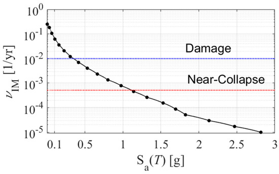
Figure 2.
IM hazard curve with IM levels and (damage and near-collapse) limit states highlighted.
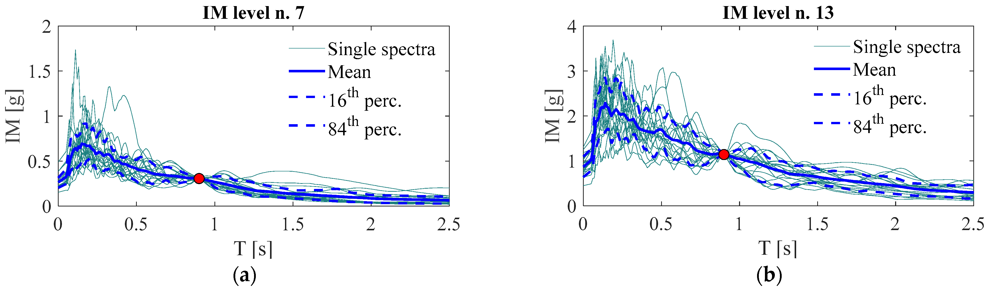
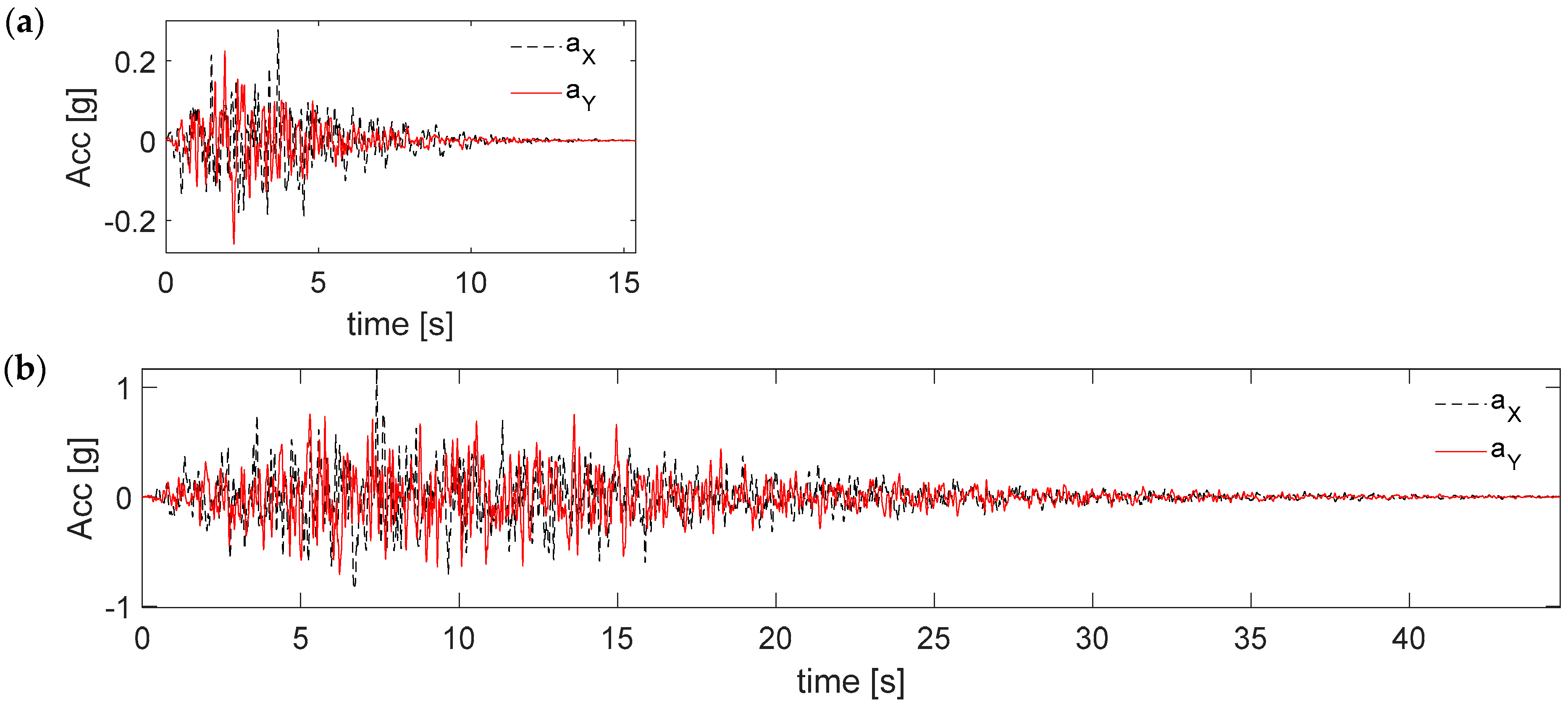
These limits stem from the current Italian seismic code (but the values comply with European Standards as well, e.g., Eurocode 0 [42]) under the assumption of a strategic role played by the bridge during its service life (note that these values are halved for ordinary constructions). The correlation between return periods and IM levels is summarized in Table 1. In order to show the features of the seismic ground motion samples used to perform probabilistic analyses, the charts in Figure 3 and Figure 4 are provided. In Figure 3, the response spectra (single components of the 20 earthquakes, average and percentiles) are provided for two IM levels with a return period close to the reference Limit States; the conditioning on the target IM is highlighted through red markers. In Figure 4, pairs (X and Y) of accelerograms selected for the two aforementioned IM levels are shown.

Table 1.
Return periods (in years) corresponding to the 20 IM levels.
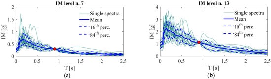
Figure 3.
Response spectra of the ground motion samples conditional to two different IM levels: (a) IM 7 (83 years return period) and (b) IM 13 (2200 years return period). Red dots identify the conditioning IM value.

Figure 4.
Pairs of ground motion components (X-Y) selected at two different IM levels: (a) IM 7 (83 years return period) and (b) IM 13 (2200 years return period).
2.2. Fragility Functions
Among the different probabilistic tools currently available, Multiple-Stripe Analysis (MSA) [41,43] is selected in this paper due to its efficiency and accuracy in building seismic demand models (e.g., models relating IM values to structural response values D). In more detail, based on the outcomes of the extensive parametric study performed in [41], and in order to achieve a level of accuracy comparable to that of robust direct simulation methods (i.e., Monte Carlo-like methods), the following setup of analysis is adopted:
- the IM hazard curve is discretized in 20 IM levels equally spaced in the log–log plane, thus MSA analysis is performed at 20 stripes;
- a set of 20 pairs (two horizontal components) of ground motion samples is used at each IM level, for a total amount of analysis equal to 400 for every case study; this setting reveals essential to properly account for the record-to-record variability typical of real earthquakes (i.e., ground motion features variability with the seismic intensity [44]);
- IM hazard curve truncation at sufficiently low MAF levels (i.e., 10–5 year−1), with the aim of accounting for the seismic intensity variability through a properly wide interval of IMs, ranging from frequent to rare seismic events.
Once data are collected from MSA analysis, Fragility functions can be analytically determined. It is recalled that, according to its usual definition [45], a seismic fragility function expresses the probability that an undesirable event will occur as a function of the value im assumed by the random value IM. In the following subsections, fragility function computation will be widely discussed based on both classical and innovative approaches.
2.2.1. Fragility Functions (Classic)
A limit state is described by a set of thresholds relevant to different potential failure modes (e.g., ductile or fragile crisis of an element, etc.). Different limit states (sets of thresholds) can be of interest, according to different performance levels of the structure, e.g., serviceability or ultimate (collapse) conditions. Therefore, failures could occur in different components and concern different response parameters and thresholds exceedance (limit states).
Each structural element can be assessed to evaluate if a given limit state is reached, and a classic definition of the fragility function can be used for this aim:
which expresses the probability of a response parameter D exceeding a limit threshold value d* identifying the passage from a functional/safe condition into a compromise/unsafe condition. For instance, in a bridge, D might represent the bearing maximum displacement demand and the corresponding end-stroke, after which the deck loses its vertical support.
Classic fragility functions can be defined according to Equation (1) for any relevant failure mode and for any limit state of interest. So, if different failure modes are considered then the fragility function characterizing the global failure of the system, , can be defined as the probability of their union, i.e.,
which is also equal to the maximum probability observed on the single failure modes.
The fragility functions defined above (Equations (1) and (2)) represent classic typologies commonly adopted to perform seismic vulnerability analysis of bridges.
Two novel typologies have recently been proposed [22] to provide a wider spectrum of information on the possible failure mechanisms, their interaction and extent. These are examined in the following subsections.
2.2.2. Fragility Functions of Concurrent Failure Mechanisms
Being a multi-component system, a bridge can manifest diverse damage mechanisms involving different structural elements and these can combine to produce a variety of damage scenarios. For instance, a seismic event might produce the attainment of the ultimate conditions on both piers and bearings; thus, one might be interested in quantifying the likelihood associated with such a combined failure event, in particular expressing its probability conditional to a given intensity level (IM = im). Such a particular type of fragility function can be mathematically expressed as follows:
where (with ) is one of the potential failure scenarios including one or more damage mechanisms. In other terms, are disjoint partitions of the global failure set, , and the probability of the latter, , is given by the sum .
2.2.3. Damage Extent Fragility Functions
Additional information we might be interested in retrieving is related to the extent of a specific failure mode; indeed, while performing seismic losses analysis, it would be useful to know the effective number/percentage of components showing a given degree of damage or exceeding a specific performance level, because this will guide and make us more aware of the reconstruction/repair cost assessment.
If we analyze a single failure mode (e.g., piers slight damage attainment) identifying it as event E, partitions of E, e.g., subsets , i = 1…, can be defined to represent failures occurring in 1, 2, … all elements belonging to the same family.
Sometimes, rather than creating partitions for individual elements, it might be convenient to work with percentages of the elements of the family (e.g., less than 30%, from 30% to 60%, and so on), thus creating rougher partitions , i = 1…, with .
Therefore, subsets of disjoint events can be considered as follows.
For example, if we assume the following partitions of the event E, , the resulting disjoint events are ,, .
Obviously, the probability of can be retrieved by summing up the probabilities of all the identified sub-events.
Starting from the above assumptions, the following two types of fragility functions will be adopted in this work:
provides the conditional (to the seismic intensity) probability of having a specific subset (e.g., between 70% and 100% according to of the previous example) of elements (e.g., piers) failed;
provides the conditional probability of a specific damage condition (e.g., 70% damaged elements).
2.3. Annual Failure Rates
Once both the hazard and the fragility are characterized, it is possible to proceed with the estimation of the mean annual failure rate, , i.e., the mean annual rate of exceedance of a given failure event E. For instance, the failure event E might be represented by the attainment of the collapse limit state for a combined damage scenario involving piers and bearings simultaneously (using fragility function of the type of Equation (3); or the attainment of a serviceability condition on the link bars according to one of the possible shades of analysis: at least one link damaged (using fragility of Equation (1)), a given percentage of them damaged (fragility of Equations (6) and (7)) and so on.
The estimation of follows from the application of Total Probability Theorem [41] and stems from the following convolution integral
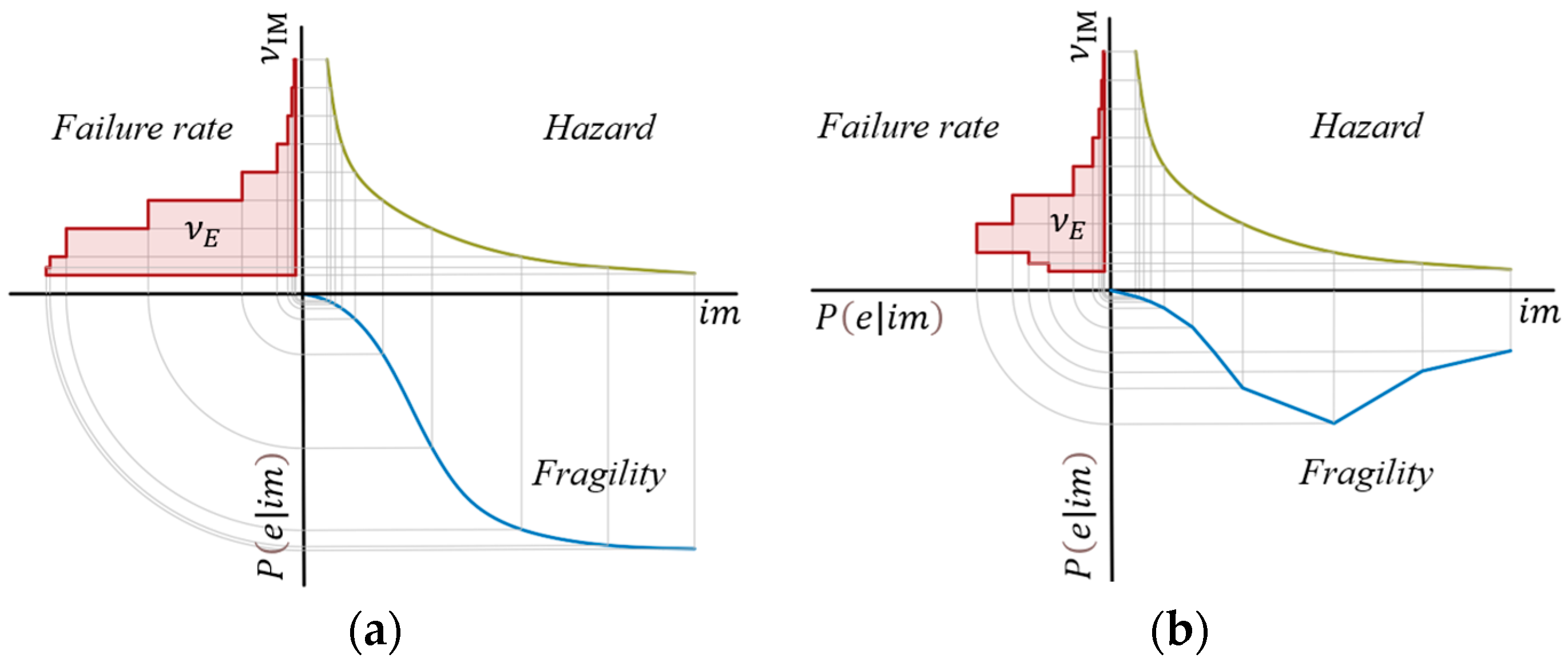
between fragility function (any of the proposed ones) and seismic hazard νIM(im). The above integral can be easily solved numerically, as graphically shown in the charts of Figure 5, which provide visual representations of the convolution between hazard (yellow curve) and fragility (blue curve) performed via the rectangular numerical integration technique (proposed for its simplicity). It is worth noting how fragility functions do not need to be monotonic within their domain of definition (as we are used to when classic fragility is adopted) but convolution can be performed regardless of this, as specifically shown in the explicative chart of Figure 5b where a non-monotonic fragility is assumed. This is important because the proposed fragility functions (Equations (3), (6) and (7)) can be notably non-monotonic because of the particular type of information they carry.
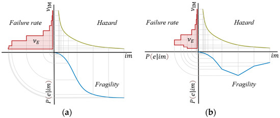
Figure 5.
Graphical representation of the convolution integral performed numerically (rectangle approximate method) to estimate annual failure rates using (a) monotonic and (b) non-monotonic fragility functions.
3. Case Studies
3.1. Considered Bridge Geometries
Link slab (LS) r.c. bridges represent a fairly typical structural typology within the infrastructural networks of many countries worldwide, especially in Italy.
The geometries of the case studies investigated in this study were selected on the basis of the most recurrent geometries observed on two major motor routes located in the Marche region, i.e., the SS76 and SS77 roads.
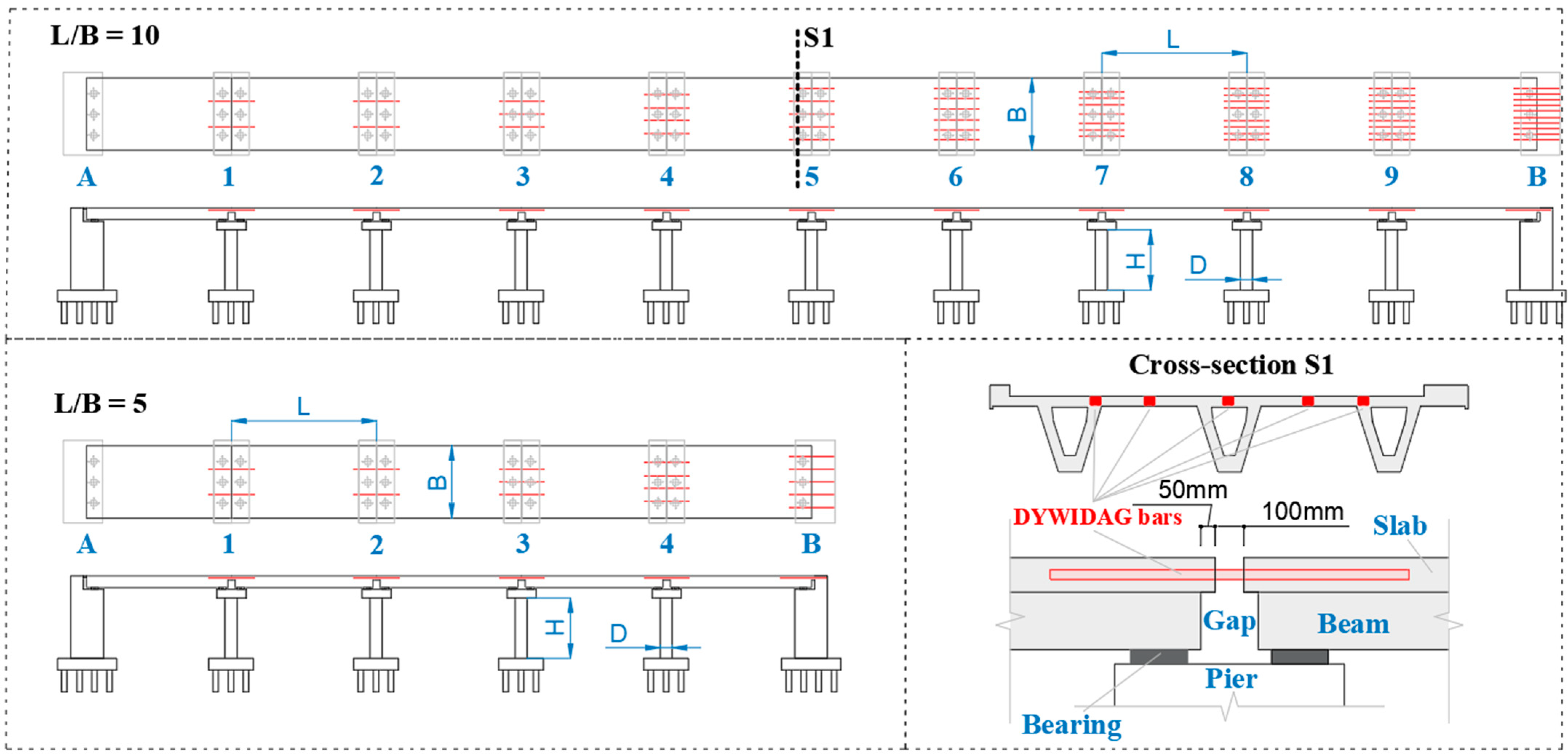
The analysis of the dataset on the SS76 and SS77 showed that the most frequent numbers of spans are N = 5 and N = 10, with a mean span length Ls = 25 m and a deck width B = 12.50 m. Based on the above, the choice of considering the following two L/B ratios: L/B = 10 (with total bridge length L = 131.0 m and N = 5), L/B = 20 (with L = 263.5 m and N = 10). To complete the set of case studies, besides the two L/B ratios, the H/D ratio (H being the pier height and D the corresponding diameter) is also assumed to parametrically vary within a reasonable range of values: H/D = 3, H/D = 5, H/D = 7. From the combination of the aforesaid cases, six multi-span link slab r.c. bridges characterized by different total lengths and pier slenderness are considered and analyzed in this study.
The deck cross-section is assumed to be B = 12.50 m wide and composed of a cast-in-site slab supported by three V-shape pre-stressed concrete girders (Figure 6). Single piers with circular cross sections are considered. These features are common to all the selected case studies.
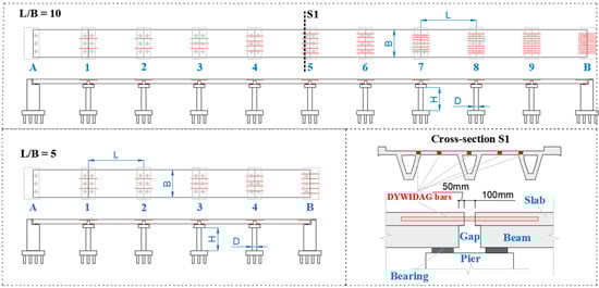
Figure 6.
Long and short bridge case studies show the link bar arrangement at the slab level and a representative transverse cross-section of the deck.
3.2. Design Properties
Each case study is conceived to be representative of existing Italian bridges constructed between 1970 and 1980, i.e., in the interval prior to the enforcement of proper specific seismic design codes. To this aim, a simulated design was carried out preliminarily on the whole set of bridges considering both gravity and seismic loads according to old Italian codes [46,47].
A simple cantilever static scheme is assumed for the seismic design of piers, with an equivalent punctual seismic force (7% of the gravity loads according to [46,47]) applied on the top. Gravity loads derive from the deck self-weight and superstructure permanent loads (approximately 50 kN/m).
Consistent with the bridge typology, spans are longitudinally connected, in correspondence with the joints and at the slab level, through kinematic links realized by means of DYWIDAG bars. These are designed considering the cumulative contributions of the seismic forces transmitted by the spans: abutment B is assumed as fixed, thus with a link slab designed to withstand the seismic mass of the whole kinematic chain (made of all the spans of the bridge), therefore at this joint, the number of link bars is the highest; on the contrary, an expansion joint is assumed in correspondence of abutment A, where there are no links; all the intermediate joints (on piers) have a number of link bars which is scaled depending on the specific location within the chain, i.e., bars number reduces moving from abutment B towards abutment A.
Material properties (Table 2) are assumed as follows: concrete grade Rck300 (i.e., cubic characteristic strength 30 MPa), stirrups and longitudinal rebars steel grade FeB44k (i.e., yielding strength 435 MPa), link DYWIDAG bars made of harmonic steel with peak strength 950 MPa.
Table 2.
Steel and concrete mechanical properties.
Features stemming from the simulated design process are summarized in Table 3 (piers design properties) and Table 4 (DYWIDAG link bars design properties at every structural joint).
Table 3.
Piers design properties for different H/D ratios.
Table 4.
Joint design properties (number and diameter of DYWIDAG bars) for different H/L ratios.
Neoprene bearings are placed between each beam and the pier cap (or abutment); related properties are as follows [48]: bearing area = 157.5 cm2, thickness = 52 mm and shear modulus = 1 MPa.
Schematic bridges representation (longitudinal prospective view, planar view and cross sections) are shown in Figure 6. Note that structural details of link slabs are taken from the design documents of a real existing bridge built in the 1980s [45].
3.3. OpenSees Numerical Model
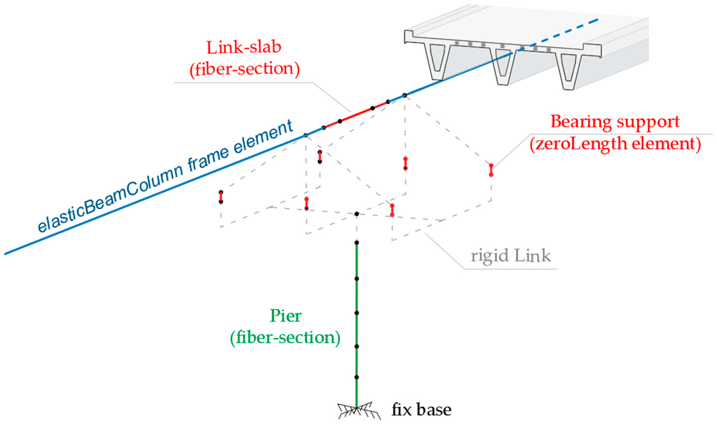
All the case studies were modeled in OpenSees [49] following the strategy described below and schematically represented in Figure 7.
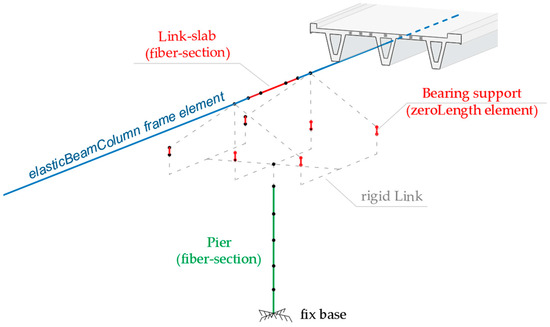
Figure 7.
Numerical model details.
Bridge models are 3D and account for both mechanical and geometrical nonlinearity. Deck girders are not expected to show nonlinear responses and are thus modeled through elastic frames. The kinematic links at the joints are explicitly modeled to reproduce the scheme shown in Figure 6, with a central bare portion of the DYWIDAG bar and two lateral parts embedded within the concrete slabs. This detail is realized in OpenSees adopting a straight layer of fibers with Steel02 uniaxial material for the DYWIDAG bars and the Concrete01 uniaxial material for the slab in the side portions. A bilinear contact element (see [50]) is adopted to account for the potential pounding between adjacent spans, assuming a gap distance in compression equal to 40 mm; in particular, such a phenomenon is expected after the link bar failure, which is explicitly accounted by the model thanks to the implementation of a MinMax material, i.e., a fictitious material wrapping the bars constitutive law that deactivates the DYWIDAG elements once attained their ultimate strain capacity. An analog contact material is inserted to catch the pounding between the deck and the abutments.
Zero-length elements with Steel01 uniaxial material are used to model the neoprene bearings [51], assuming an elastic stiffness and a maximum admissible strength equal to the lower value between the friction resistance (where is the vertical load transmitted on the bearing, and = 0.25 is the friction coefficient between concrete and neoprene surfaces), and the shear strength (assuming is the ultimate shear strain of the neoprene pads).
Distributed plasticity with fiber sections is used for the piers, with the Concrete01 material set according to Mander [52] in order to simulate both confined and unconfined portions (i.e., parts within and outside the hoops, respectively). Pier steel reinforcements are also modeled using fibers exploiting the Steel02 uniaxial material. Pier caps are modeled as rigid.
Regarding the abutments, a classic seat type resting on piles is considered.
The interaction between abutments and soil is considered following validated strategies available in the literature, briefly recalled below. Along the longitudinal direction, bridge motions inducing compression of the soil behind the abutment backwall produce, as the main effect, the development of a passive resistance within the soil, and this is simulated using the hyperbolic model proposed by Shamsabadi et al. [53] for a granular soil type. Longitudinal movements of the bridge away from the abutment generate (active) forces mainly withstood by piles, and this response can be simulated through a trilinear force deformation law [54]. A similar behavior is expected along the transverse direction hence the same model is used. Each of the aforesaid (passive/active) constitutive laws is implemented through a proper set of zero-length elements.
It is worth mentioning that, in this work, neither the influence of asynchronous seismic inputs nor soil–structure interaction effects under the piers are taken into account, but refinements would be possible (e.g., [55,56]) provided that a proper knowledge of the geotechnical conditions of the soil is reached.
3.4. Limit States and Capacity Thresholds
Based on the main failure mechanisms expected on the bridge, a set of relevant response parameters is selected to be monitored during numerical simulations and post-processed through the proposed probabilistic framework.
The failure modes potentially occurring are on piers (according to shear and/or flexural crisis), bearings, links, and abutments. In light of this, capacity thresholds are determined for each of these structural components and for two different limit states (LSs): a damage onset limit state (simply referred to as damage LS hereinafter) and a near collapse LS (collapse hereinafter). Threshold values summarized in Table 5 are derived in part from the literature [54,57] (abutment capacity), and in part from seismic codes and relevant technical documents [51,58] (bearings and piers limits). Thresholds adopted for the link bars directly follow the constitutive law of this specific steel grade.
Table 5.
Limit states and capacity thresholds of different structural subcomponents.
It must be noted that the limit values for piers are expressed in terms of top displacements because it is easier to track this response parameter during the analysis. However, preliminary moment–curvature sectional analyses were performed on the piers cross-section (according to a cantilever static scheme) in order to correlate the damage level (plastic hinge at the base) to the proper values of the pier top displacement.
4. Failure Rate and Result Discussion
This section collects the main outcomes stemming from the probabilistic analysis. Results are presented in terms of fragility functions and mean annual rates of exceedance considering two limit states, i.e., damage onset LS (corresponding to TR = 100 years, ν = 1 × 10⁻² 1/year) and collapse LS (corresponding to TR = 1950 years, ν = 5 × 10⁻⁴ 1/year).
The results presentation is organized as follows. The bridge with L/B = 10 (the longest) and H/D = 5 (intermediate pier slenderness) is assumed as a reference case study and a detailed discussion on the seismic vulnerability and reliability of this system is provided in the next subsections: failure rates derived from classic element-based fragility functions (Section 4.1), failure rates derived from combined failure mechanisms (Section 4.2), failure rates related to different damage extent scenarios (Section 4.3).
Finally, a comparison among the failure rates associated with different bridge geometries is presented and thoroughly discussed in Section 4.4.
4.1. Failure Rates from Classic Element-Based Fragility Functions
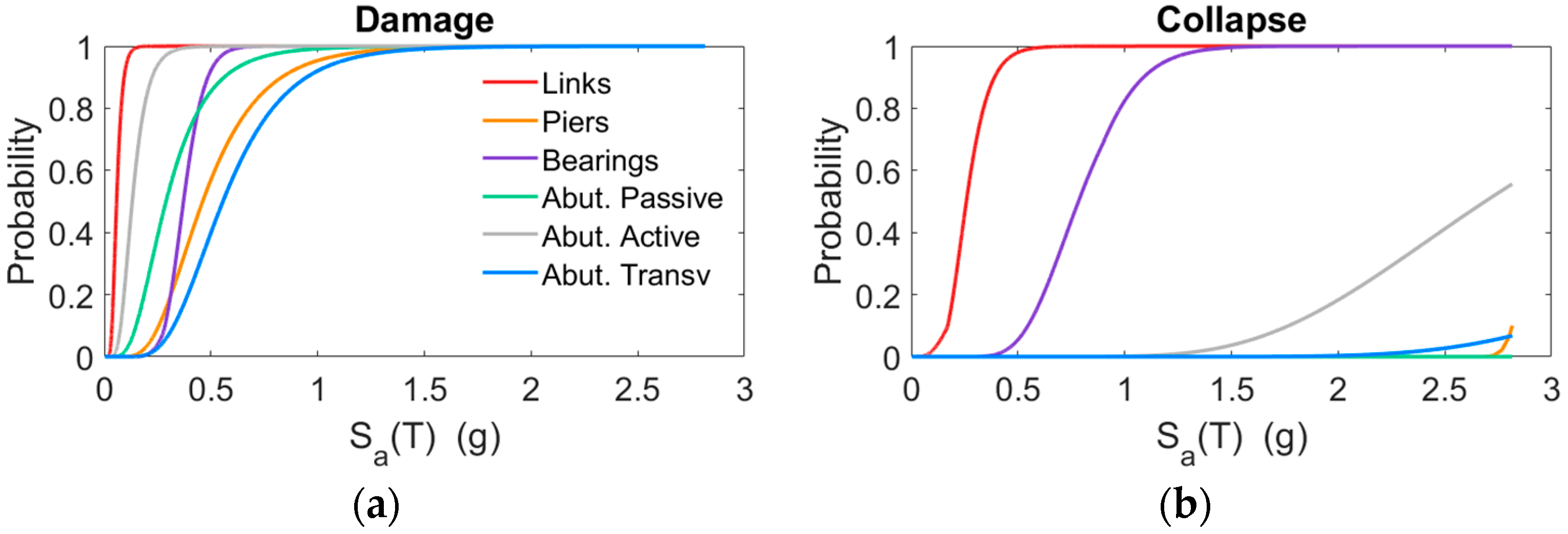
First, classic fragility curves are presented in Figure 8 to provide a global overview of the different vulnerabilities shown by the bridge at the damage and collapse limit states. The considered failure mechanisms are those presented in Section 3.4 and involve the structural elements here briefly recalled: Link bars, Piers, Bearings, and Abutments. The latter can show three different failure modes, related to longitudinal active or passive response and transversal response.
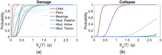
Figure 8.
Fragility curves for different elements and failure modes evaluated for two limit states: (a) damage, (b) collapse.
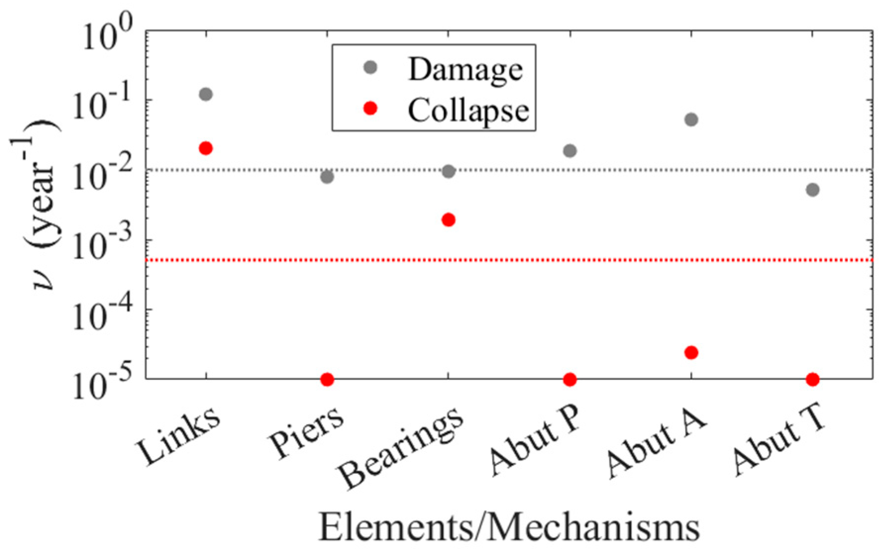
The annual rates of exceedance associated with each of the aforementioned failure modes (obtained through the convolution between fragility and hazard functions) are collected in the chart of Figure 9. Markers with different colors identify damage (grey) and collapse (red) failure rates. Using the same colors, two horizontal dotted lines are superimposed on the chart to identify the code-based MAFs corresponding to the considered limit states (ν = 1 × 10⁻² 1/year for damage LS, ν = 5 × 10⁻⁴ 1/year for collapse LS). Quantitative assessment of the reliability of the system can be carried out by comparing the obtained failure rate values with the reference MAF levels defined by the codes; in particular, annual rates above the line corresponding to the code-based MAF denote “unsafe” conditions, while annual rates below the line identify “safe” situations; the vertical distance between the marker and the line is a measure of the safety margin against that specific mode of failure.

Figure 9.
Annual failure rates for different elements and failure modes at damage and collapse LSs.
In light of this, the outcomes presented in Figure 9 can be interpreted as follows:
- at the collapse limit state, piers and abutments (and all related mechanisms) show satisfactory safety margins, while bearings and links manifest failure rates higher than desired (slightly higher for bearings, notably higher for links);
- at the damage limit state, all the elements/mechanisms present rates of exceedance which are, on average, around the target MAF value, except for the markers of links and abutment active response which are above the reference line.
It shall be noted that these results might be not sufficient to provide a clear understanding of the level of vulnerability of the bridge, because information on the extension of the damage is missing. Indeed, failure rates stemming from classic fragility functions refer to the occurrence of at least one unsatisfactory event and thus any detailed evidence concerning the number of elements experiencing damage is totally hidden. To complete this information, one should refer to Section 4.3, where the novel fragility functions are used to estimate the risk related to different damage extent scenarios.
4.2. Failure Rates Associated with Different Damage Mechanisms Combination
In order to enrich the level of information concerning the specific vulnerabilities of the bridge, fragility analysis is performed using the novel approach defined by Equation (3), capable of quantifying the probability (conditional to seismic intensity levels) of occurrence of multiple failure modes (i.e., groups of mechanisms activated simultaneously).
Fragility curves for different subsets of failure scenarios are presented in Figure 10 for both damage and collapse limit states. This type of fragility analysis is useful (even before moving to the next step of risk estimation) because useful insights can be retrieved concerning the group of damage mechanisms most representative of different intervals of seismic intensity. For instance, looking at the collapse limit state (Figure 10b), it can be observed how the range of IMs approximately from 0.2 g to 0.75 g is governed by link-only related failures, while at the higher intensities both bearings and links failures are predominant. An additional fragility type, labeled as Global, is reported in Figure 10, and it is given by the sum, im-by-im, of the probabilities related to the different damage scenarios. This fragility can be also seen as the envelope of the classic ones presented in the previous Section 4.1 (Figure 8).
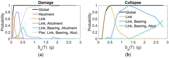
Figure 10.
Fragility curves for different damage mechanism combinations evaluated for two limit states: (a) damage, (b) collapse.
The annual rates of exceedance associated with each of the aforementioned failure mode combinations are collected in the chart of Figure 11. The combined damage scenarios are identified with capital letters denoting the initials of the names of the involved elements (e.g., PLBA = Piers–Links–Bearings–Abutments; LB = Links–Bearings, and so on). The risk estimates related to Global fragility are also shown in the chart using a colored asterisk as a marker and are labeled as Global. It is worth noting that the failure rates presented in this chart are always lower or at maximum equal to those presented in the previous subsection, simply because they refer to mutual partitions of the failure.
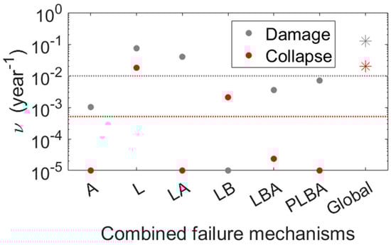
Figure 11.
Annual failure rates for different failure mode combinations at damage and collapse LS.
4.3. Failure Rates Associated with Different Damage Extension Scenarios
In this section, the analysis of the vulnerability and risk is pushed a little bit further. Information about the extension of the failure mechanisms identified on each structural element is indeed provided, first in terms of fragility curves (derived according to Equations (6) and (7)) and then in terms of annual rates of exceedance.
Results are presented separately for the three main families of structural elements, i.e., Bearings (Figure 12), Links (Figure 13), and Piers (Figure 14).

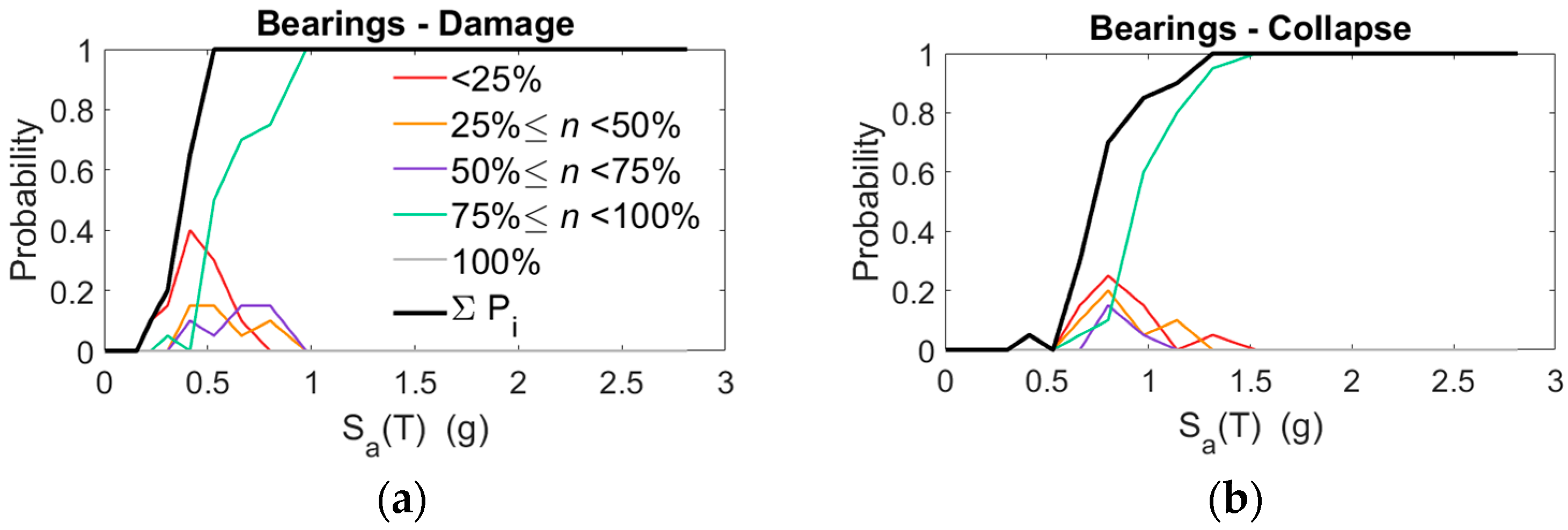
Figure 12.
Fragility curves for different percentages of damaged bearings, evaluated for two limit states: (a) damage, (b) collapse.
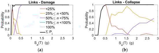
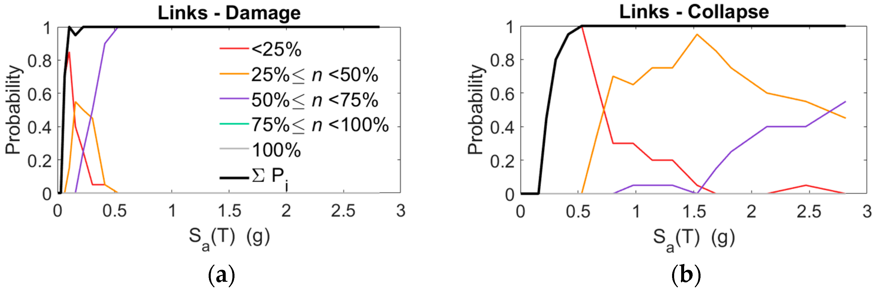
Figure 13.
Fragility curves for different percentages of damaged link–bars, evaluated for two limit states: (a) damage, (b) collapse.
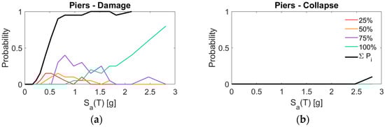
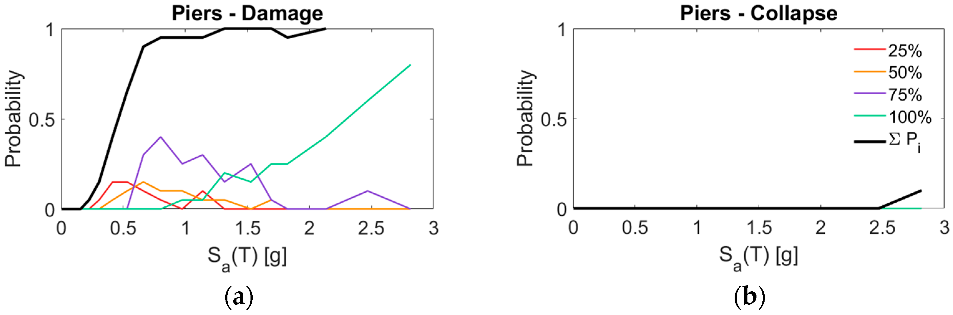
Figure 14.
Fragility curves for different percentages of damaged piers, evaluated for two limit states: (a) damage, (b) collapse.
Different percent intervals of damage extent are considered. Besides the fragility curves of each percentage range, the curve obtained by summing up all the single curves is superimposed with a solid black line, and this corresponds to the classic fragility curve of each element already presented in Figure 8 of Section 4.1. The only difference between the classic curves presented in Figure 8 and the current one in Figure 12, Figure 13 and Figure 14 is in the lognormal assumption used only to compute the ones in Figure 8. However, apart from the different degrees of smoothness, these curves carry the same identical information on the global damage probability of single structural elements.
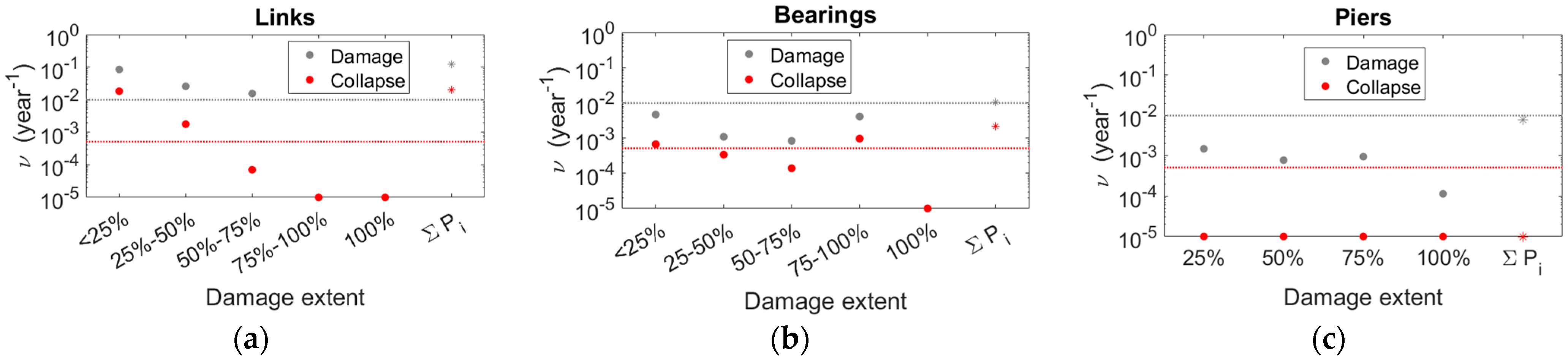
The annual rates of exceedance are presented in Figure 15 in separate charts, one dedicated to each structural element. Damage and Collapse failure rates are compared using the usual legend of colors and symbols.
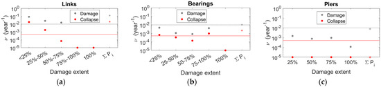
Figure 15.
Annual failure rates for different damage and collapse extent scenarios involving: (a) links, (b) bearings, (c) piers.
The main conclusions drawn from these outcomes are listed below:
- regarding the failure rates of the link bars, it can be observed how the fairly high level of collapse risk previously identified in Section 4.1 actually involves a very small number of elements (less than 25%), and this information notably helps to adjust this result interpretation, which, based on the sole numbers provided in Figure 9, may appear greater than it really is.
- It can be seen how the risk decreases rapidly as we look at higher damage extent scenarios, e.g., the MAF of having ruptures on 25–50% of links is one order of magnitude lower than the MAF of having less than 25% of elements failed.
- Similar comments can be made for other structural elements.
4.4. Failure Rates Sensitivity to Different Bridge Geometries
To conclude, the failure rate sensitivity to the different examined bridge geometries is assessed. Due to space constraints, it is not possible to maintain the previous level of detail in the results presentation of every case study. A comparison among the risk values obtained from different bridges is proposed in the charts of Figure 16. Different markers identify different bridges, according to the legend in Figure 16f; colors identify the limit state (as before). The analysis of the outcomes leads to the following main comments:
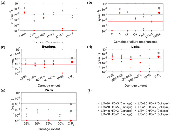
Figure 16.
Annual failure rates comparison among bridges with different geometries: (a) single-element failure rates; (b) failure mechanism combinations; (c) failure rates on bearings; (d) failure rates on links; (e) failure rates on piers; (f) legend of case studies.
- Overall, single-element failure rates (Figure 16a) of different bridges do not vary significantly and the estimated MAFs remain relatively constant.
- A higher variability is observed on the annual rates characterizing different failure mechanism combinations (Figure 16b), which are however expected to change from case to case; in particular, this variability is higher at the damage LS and quite negligible at the collapse LS.
- More specifically (Figure 16d), the longest bridge (L/B = 20) is the only one that shows a different trend of MAF values, and this trend testifies that the probability of link failure is higher but involves a limited number of elements; on the contrary, shorter bridges have a higher probability of more widespread links disruptions.
- Regarding the piers, all the bridges show proper safety margins against the collapse, while the damage extent scenarios at the damage limit state are characterized by MAF values with a certain degree of variability.
5. Conclusions
A comprehensive probabilistic framework is proposed and adopted in this study to perform seismic reliability and risk analysis of existing link slab (LS) bridges, which represent a widely diffused structural typology within the infrastructural networks of many countries.
The methodology is extensively presented in the former part of the paper in order to highlight the novelty and the strengths with respect to classic seismic vulnerability analysis.
The main difference with respect to the common approaches relies on the types of fragility functions adopted: the ones adopted in this study are capable of retrieving more specific and detailed information on the possible failure modes, without limiting the analysis to the global failure conditions while also considering several intermediate damage scenarios (including one or more damage mechanisms) and providing insights on the numerosity of elements involved within a given damage scenario.
A set of case studies is presented, consisting of Link-Slab reinforced concrete bridges with different geometries, which were preliminarily designed according to the codes enforced during the 1970s, modelled in OpenSees and then subjected to reliability analyses exploiting the proposed probabilistic framework.
According to outcomes stemming from the study, it is observed that the main failure mechanisms characterizing this bridge typology involve the link bars and the bearings.
The former represents the peculiarity of these systems, introduced to exploit several advantages in terms of driving comfort (reduced number of expansion joints) and functionality (hyperstaticity under horizontal actions and simply supported beam scheme under gravity loads). At the same time, these elements might represent a primary source of vulnerability; indeed, annual failure rates much higher than expected are observed. However, thanks to a refined fragility analysis, it was possible to further investigate the entity of the problem in terms of damage extent. It was observed how the higher failure rates are actually related to the disruption of a very limited number of links (less than 25%), while the collapse probabilities associated with more widespread damages are lower and comparable to the reference-expected hazard level at the collapse limit state.
Regarding the failure rates of bearings, it is realistic to have MAF values higher than the code limit considering that neoprene pads commonly adopted in existing bridges were not designed to withstand earthquakes and the rubber property is not comparable to that of modern devices and isolators. This vulnerability could be removed by replacing the old supports with newer and more suitable ones.
Piers, despite being designed with simplified seismic rules, were revealed to have proper safety margins against the collapse. Such main results hold (with minor variations) for all the bridge geometries investigated.
Besides these results being specifically related to the examined case studies, the following general comments on the methods can be made.
The proposed strategy was revealed to be suitable to provide a higher level of information on the reliability of the systems because it allows the association of different levels of risk (hence safety margins) to failure scenarios which differ in terms of elements/mechanisms involved and damage extension. Such a higher level of detail in the risk analysis may be useful to better quantify post-earthquake consequences (e.g., costs and losses) and define more tailored retrofit interventions, which are outside the scope of the present work but are considered worth mentioning.
Moreover, the proposed probabilistic framework is made of different components, namely: (1) a stochastic ground motion model for hazard characterization and ground motion sample generation; (2) the multiple stripe analysis with proper parameter setup aimed at providing accurate estimates of the risk; (3) innovative fragility functions. Each of these tools was carefully chosen and set in order to make the framework reliable and robust and offer the reader a suitable reference framework for performing risk analysis.
In future development, the proposed strategy will be used to assess the vulnerability and risk of other widespread bridge classes, such as integral bridges, post-tensioned precast bridges or more modern typologies such as steel–concrete composite bridges or bridges with seismically isolated decks.
Author Contributions
Conceptualization, F.S.; methodology, F.S. and L.M.; software, L.M.; validation, F.S.; formal analysis, F.S. and L.M.; investigation, F.S. and L.M.; resources, F.S.; data curation, F.S. and L.M.; writing—original draft preparation, F.S. and L.M.; writing—review and editing, F.S. and L.M.; visualization, F.S. and L.M.; supervision, F.S. All authors have read and agreed to the published version of the manuscript.
Funding
This research received no external funding.
Institutional Review Board Statement
Not applicable.
Informed Consent Statement
Not applicable.
Data Availability Statement
The database of synthetic seismic ground motions used in this work is made available upon request to the corresponding author (fabrizio.scozzese@unicam.it).
Conflicts of Interest
The authors declare no conflict of interest.
Appendix A. Details on Seismic Hazard and Ground Motion Model
The seismic scenario is described by a source model characterized by two main random seismological parameters, namely the moment magnitude M and the epicentral distance R. A Gutenberg–Richter recurrence law is used to describe the magnitude–frequency relationship of the seismic source:
in which the parameter a accounts for the mean number of earthquakes expected from the seismic source, while the parameter b is a regional seismicity factor governing the proportion of small to large earthquakes. The assumed recurrence law, bounded within the range of magnitudes of interest [m0, mmax], leads to the following probability density function (PDF) of the moment magnitude:
being β = b* loge(10), m0 the magnitude value below which non-significant effects are expected on the structures, and mmax the physical upper bound of the magnitudes expected from the source. In this application, it is assumed m0 = 5.5, mmax = 8, a = 4.35 and b = 0.9, in order to provide a seismic hazard representative of Italian medium-high seismicity zones. The epicentral distance is modeled according to the following PDF:
which is obtained under the hypothesis that the source produces random earthquakes with equal likelihood anywhere within a distance from the site rmax = 100 km, beyond which the seismic effects are assumed to become negligible. The soil condition is described by a deterministic value of the shear-wave velocity parameter VS30 = 255 m/s, representative of deformable soil condition.
The Atkinson-Silva [40] source-based ground motion model is used to describe the attenuation from the source to the building site. This model, combined with the stochastic point source simulation method of [39] is employed to generate synthetic accelerograms consistent with the random variables characterizing the seismic scenario, i.e., mainly magnitude M and source-to-site distance R.
For the simulation of two horizontal ground motion components, the stochastic model of [39] is modified as suggested by [59], according to which the radiation spectra can be considered to have the same shape for the two horizontal orthogonal directions, but the intensities are scaled by two different scaling random parameters (random scaling disturbance ε1, ε2) generated as samples of a multivariate lognormal distribution with zero mean, standard deviation σ = 0.523 and correlation ρ = 0.8. This way, the target radiation spectra along directions 1 and 2 will be equal to A1(ω) = ε1A(ω) and A2(ω) = ε2A(ω).
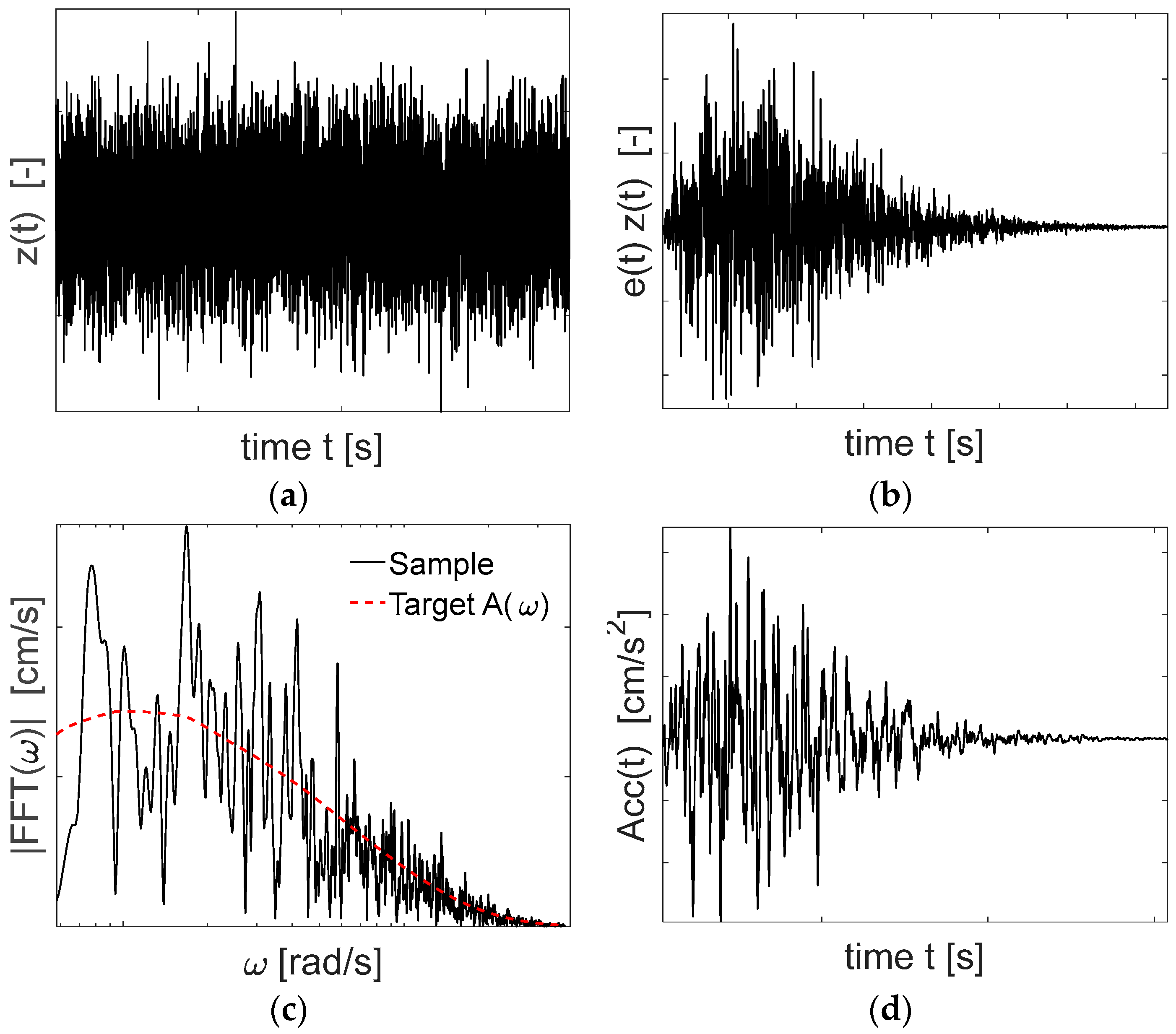
The random scaling disturbance (ε1,ε2), together with the Gaussian white noise process ensures the ground motions record-to-record variability to be accounted for. In particular, for each earthquake sample a Gaussian white noise signal is generated (Figure A1a) and, after being windowed through the envelope functions e(t) (Figure A1b), its normalized frequency spectrum is applied to the target radiation spectrum (Figure A1c), thus providing the variability of the energy content within the frequency domain. Such variability is further amplified by the lognormally distributed multiplicative factors (ε1,ε2) of the radiation spectra. The resulting sample of acceleration time series is finally generated by back-transforming the spectrum from the frequency to the time domain (Figure A1d).
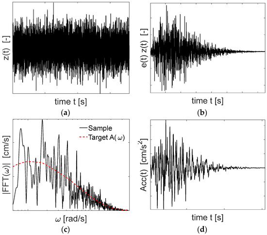
Figure A1.
Main steps of the point-source stochastic ground motion simulation method: (a) white noise generation; (b) time modulation; (c) Fourier transformation and filtering in the frequency domain; (d) inverse Fourier transformation to time domain.
Figure A1.
Main steps of the point-source stochastic ground motion simulation method: (a) white noise generation; (b) time modulation; (c) Fourier transformation and filtering in the frequency domain; (d) inverse Fourier transformation to time domain.
References
- Deodatis, G.; Ellingwood, B.R.; Frangopol, D.M. (Eds.) Safety, Reliability, Risk and Life-Cycle Performance of Structures and Infrastructures; CRC Press: Boca Raton, FL, USA, 2014. [Google Scholar]
- Tubaldi, E.; Scozzese, F.; De Domenico, D.; Dall’Asta, A. Effects of axial loads and higher order modes on the seismic response of tall bridge piers. Eng. Struct. 2021, 247, 113134. [Google Scholar] [CrossRef]
- Tubaldi, E.; Dall’asta, A. A design method for seismically isolated bridges with abutment restraint. Eng. Struct. 2011, 33, 786–795. [Google Scholar] [CrossRef]
- Shekhar, S.; Ghosh, J. Improved Component-Level Deterioration Modeling and Capacity Estimation for Seismic Fragility Assessment of Highway Bridges. ASCE-ASME J. Risk Uncertain. Eng. Syst. Part A Civ. Eng. 2021, 7, 04021053. [Google Scholar] [CrossRef]
- Kilanitis, I.; Sextos, A. Integrated seismic risk and resilience assessment of roadway networks in earthquake prone areas. Bull. Earthq. Eng. 2019, 17, 181–210. [Google Scholar] [CrossRef]
- Turchetti, F.; Tubaldi, E.; Douglas, J.; Zanini, M.A.; Dall’asta, A. A risk-targeted approach for the seismic design of bridge piers. Bull. Earthq. Eng. 2023, 21, 4923–4950. [Google Scholar] [CrossRef]
- Tubaldi, E.; Macorini, L.; Izzuddin, B.A.; Manes, C.; Laio, F. A framework for probabilistic assessment of clear-water scour around bridge piers. Struct. Saf. 2017, 69, 11–22. [Google Scholar] [CrossRef]
- Zampieri, P.; Zanini, M.A.; Faleschini, F.; Hofer, L.; Pellegrino, C. Failure analysis of masonry arch bridges subject to local pier scour. Eng. Fail. Anal. 2017, 79, 371–384. [Google Scholar] [CrossRef]
- Ragni, L.; Scozzese, F.; Gara, F.; Tubaldi, E. Dynamic identification and collapse assessment of Rubbianello Bridge. In Towards a Resilient Built Environment Risk and Asset Management: IABSE Symposium Guimarães; Curran Associates, Inc.: Zurich, Switzerland, 2019; pp. 619–626. [Google Scholar] [CrossRef]
- Scozzese, F.; Tubaldi, E.; Dall’Asta, A. Damage metrics for masonry bridges under scour scenarios. Eng. Struct. 2023, 296, 116914. [Google Scholar] [CrossRef]
- Poeta, A.; Micozzi, F.; Gioiella, L.; Dall’Asta, A. A case study for the reliability evaluation of an existing prestressed bridge according to current Standard. ce/papers 2023, 6, 36–42. [Google Scholar] [CrossRef]
- Mazzatura, I.; Salvatore, W.; Caprili, S.; Celati, S.; Mori, M.; Gammino, M. Damage detection, localization, and quantification for steel cables of post-tensioned bridge decks. Structures 2023, 57, 105314. [Google Scholar] [CrossRef]
- Nettis, A.; Massimi, V.; Nutricato, R.; Nitti, D.O.; Samarelli, S.; Uva, G. Satellite-based interferometry for monitoring structural deformations of bridge portfolios. Autom. Constr. 2023, 147, 104707. [Google Scholar] [CrossRef]
- Micozzi, F.; Morici, M.; Zona, A.; Dall’Asta, A. Vision-Based Structural Monitoring: Application to a Medium-Span Post-Tensioned Concrete Bridge under Vehicular Traffic. Infrastructures 2023, 8, 152. [Google Scholar] [CrossRef]
- Mazzatura, I.; Natali, A.; Salvatore, W.; Principi, L.; Morici, M.; Dall’Asta, A. A methodological proposal for the analysis of bridges inspections data according to the Italian Guidelines. ce/papers 2023, 6, 1399–1404. [Google Scholar] [CrossRef]
- De Matteis, G.; Carbonari, S.; Chisari, C.; D’Amato, M.; Mattei, F.; Zizi, M.; Braga, F.; Caprili, S.; Dall’Asta, A.; Gara, F.; et al. Nonlinear analysis procedures for safety assessment of existing RC bridges under traffic loads. ce/papers 2023, 6, 28–35. [Google Scholar] [CrossRef]
- Briseghella, B.; Siviero, E.; Zordan, T. A composite integral bridge in Trento, Italy: Design and Analysis. In IABSE Sym-Posium Report; International Association for Bridge and Structural Engineering: Zurich, Switzerland, 2004; Volume 88, pp. 297–302. [Google Scholar]
- Minnucci, L.; Scozzese, F.; Dall’Asta, A.; Carbonari, S.; Gara, F. Influence of the Deck Length on the Fragility Assessment of Italian RC Link Slab Bridges. In International Conference of the European Association on Quality Control of Bridges and Structures; Springer: Cham, Switzerland, 2021; pp. 731–739. [Google Scholar]
- Caner, A.; Zia, P. Behavior and design of link slabs for jointless bridge decks. PCI J. 1998, 43, 68–80. [Google Scholar] [CrossRef]
- Sevgili, G.; Caner, A. Improved seismic response of multisimple-span skewed bridges retrofitted with link slabs. J. Bridg. Eng. 2009, 14, 452–459. [Google Scholar] [CrossRef]
- Wang, C.; Shen, Y.; Zou, Y.; Zhuang, Y.; Li, T. Analysis of Mechanical Characteristics of Steel-Concrete Composite Flat Link Slab on Simply-Supported Beam Bridge. KSCE J. Civ. Eng. 2019, 23, 3571–3580. [Google Scholar] [CrossRef]
- Minnucci, L.; Scozzese, F.; Carbonari, S.; Gara, F.; Dall’asta, A. Innovative fragility-based method for failure mechanisms and damage extension analysis of bridges. Infrastructures 2022, 7, 122. [Google Scholar] [CrossRef]
- Nielson, B.G.; DesRoches, R. Seismic fragility curves for typical highway bridge classes in the Central and South-eastern United States. Earthq. Spectra 2007, 23, 615–633. [Google Scholar] [CrossRef]
- Ramanathan, K.; Desroches, R.; Padgett, J.E. Analytical fragility curves for multispan continuous steel girder bridges in moderate seismic zones. Transp. Res. Rec. J. Transp. Res. Board 2010, 2202, 173–182. [Google Scholar] [CrossRef]
- Mangalathu, S.; Jeon, J.-S.; Padgett, J.E.; DesRoches, R. ANCOVA-based grouping of bridge classes for seismic fragility assessment. Eng. Struct. 2016, 123, 379–394. [Google Scholar] [CrossRef]
- Shinozuka, M.; Feng, M.Q.; Lee, J.; Naganuma, T. Statistical analysis of fragility curves. J. Eng. Mech. 2000, 126, 1224–1231. [Google Scholar] [CrossRef]
- Hwang, H.; Liu, J.B.; Chiu, Y.H. Seismic Fragility Analysis of Highway Bridges; Mid-America Earthquake Center CD Release 01–06; Mid-America Earthquake Center: Chicago, IL, USA, 2001. [Google Scholar]
- Mackie, K.R.; Stojadinović, B. R-factor parameterized bridge damage fragility curves. J. Bridg. Eng. 2007, 12, 500–510. [Google Scholar] [CrossRef]
- Stefanidou, S.P.; Kappos, A.J. Methodology for the development of bridge-specific fragility curves. Earthq. Eng. Struct. Dyn. 2016, 46, 73–93. [Google Scholar] [CrossRef]
- Nielson, B.G.; DesRoches, R. Seismic fragility methodology for highway bridges using a component level approach. Earthq. Eng. Struct. Dyn. 2007, 36, 823–839. [Google Scholar] [CrossRef]
- Nowak, A.S.; Cho, T. Prediction of the combination of failure modes for an arch bridge system. J. Constr. Steel Res. 2007, 63, 1561–1569. [Google Scholar] [CrossRef]
- Gehl, P.; D’Ayala, D. Development of Bayesian Networks for the multi-hazard fragility assessment of bridge systems. Struct. Saf. 2016, 60, 37–46. [Google Scholar] [CrossRef]
- Lupoi, G.; Franchin, P.; Lupoi, A.; Pinto, P.E. Seismic fragility analysis of structural systems. J. Eng. Mech. 2006, 132, 385–395. [Google Scholar] [CrossRef]
- Gardoni, P.; Mosalam, K.M.; Der Kiureghian, A. Probabilistic seismic demand models and fragility estimates for RC bridges. J. Earthq. Eng. 2003, 7, 79–106. [Google Scholar] [CrossRef]
- Padgett, J.E.; DesRoches, R. Methodology for the development of analytical fragility curves for retrofitted bridges. Earthq. Eng. Struct. Dyn. 2008, 37, 1157–1174. [Google Scholar] [CrossRef]
- Ghosh, J.; Rokneddin, K.; Duenas-Osorio, L.; Padgett, J.E. Seismic reliability assessment of aging highway bridge networks with field instrumentation data and correlated failures, I: Methodology. Earthq. Spectra 2014, 30, 819–843. [Google Scholar] [CrossRef]
- Dueñas-Osorio, L.; Padgett, J.E. Seismic reliability assessment of bridges with user-defined system failure events. J. Eng. Mech. 2011, 137, 680–690. [Google Scholar] [CrossRef]
- Scozzese, F.; Terracciano, G.; Zona, A.; Della Corte, G.; Dall’Asta, A.; Landolfo, R. RINTC project: Nonlinear dynamic analyses of Italian code-conforming steel single-storey buildings for collapse risk assess-ment. In Proceedings of the COMPDYN 6th International Conference on Computational Methods in Structural Dynamics and Earthquake Engineering, Rhodes Island, Greece, 15–17 June 2017. [Google Scholar]
- Boore, D.M. Simulation of ground motion using the stochastic method. Pure Appl. Geophys. 2003, 160, 635–676. [Google Scholar] [CrossRef]
- Atkinson, G.M.; Silva, W. Stochastic modeling of California ground motions. Bull. Seismol. Soc. Am. 2000, 90, 255–274. [Google Scholar] [CrossRef]
- Scozzese, F.; Tubaldi, E.; Dall’Asta, A. Assessment of the effectiveness of multiple-stripe analysis by using a stochastic earthquake input model. Bull. Earthq. Eng. 2020, 18, 3167–3203. [Google Scholar] [CrossRef]
- EN 1990: Eurocode—Basis of Structural Design [Authority: The European Union Per Regulation 305/2011, Directive 98/34/EC, Directive 2004/18/EC]. 2002. Available online: https://www.phd.eng.br/wp-content/uploads/2015/12/en.1990.2002.pdf (accessed on 17 December 2023).
- Jalayer, F.; Cornell, C.A. Alternative non-linear demand estimation methods for probability-based seismic assessments. Earthq. Eng. Struct. Dyn. 2009, 38, 951–972. [Google Scholar] [CrossRef]
- Bradley, B.A.; Cubrinovski, M.; Dhakal, R.P.; MacRae, G.A. Probabilistic seismic performance and loss assessment of a bridge–foundation–soil system. Soil Dyn. Earthq. Eng. 2010, 30, 395–411. [Google Scholar] [CrossRef]
- Porter, K. A beginner’s guide to fragility, vulnerability, and risk. Encycl. Earthq. Eng. 2015, 2015, 235–260. [Google Scholar]
- Decreto Ministeriale 3 marzo 1975; Approvazione Delle Norme Tecniche per le Costruzioni in Zone Sismiche. Ministero dei Lavori Pubblici: Gazzetta Ufficiale, Italy, 1975. (In Italian)
- Decreto Ministeriale 3 maggio 1972; Norme Tecniche Alle Quali Devono Uniformarsi le Costruzioni in Conglomerato Cementizio, Normale e Precompresso ed a Struttura Metallica. Ministero dei Lavori Pubblici: Gazzetta Ufficiale, Italy, 1972. (In Italian)
- CNR (Consiglio Nazionale delle Ricerche). Apparecchi di Appoggio per le Costruzioni; Istruzioni per L’impiego (CNR 10018), Rome; Consiglio Nazionale delle Ricerche: Bollettino Ufficiale Parte IV Norme Tecniche n. 190 del 21 dicembre 1999; CNR: Rome, Italy, 1999. (In Italian) [Google Scholar]
- McKeena, F.; Fenves, G.; Scott, M. Open System for Earthquake Engineering Simulation (OpenSees); Pacific Earthquake Engineering Research Center (PEER), University of California: Berkeley, CA, USA, 2015. [Google Scholar]
- Muthukumar, S.; DesRoches, R. A Hertz contact model with non-linear damping for pounding simulation. Earthq. Eng. Struct. Dyn. 2006, 35, 811–828. [Google Scholar] [CrossRef]
- DSTE/PRS & UNIBAS—Autostrade per l’Italia S.p.A. Manuale utente della procedura AVSper la valutazione della vulnerabilità e rischio sismico dei ponti eviadotti autostradali. In Verifiche Sismiche NTC 2018—V01; Version 2.1; DSTE/PRS: Rome, Italy, 2019. [Google Scholar]
- Mander, J.B.; Priestley, M.J.; Park, R. Theoretical stress-strain model for confined concrete. J. Struct. Eng. 1988, 114, 1804–1826. [Google Scholar] [CrossRef]
- Shamsabadi, A.; Rollins, K.M.; Kapuskar, M. Nonlinear soil–abutment–bridge structure interaction for seismic performance-based design. J. Geotech. Geoenviron. Eng. 2007, 133, 707–720. [Google Scholar] [CrossRef]
- Seismic Design Criteria; California Department of Transportation (CALTRANS): Sacramento, CA, USA, 2015.
- Capatti, M.C.; Tropeano, G.; Morici, M.; Carbonari, S.; Dezi, F.; Leoni, G.; Silvestri, F. Implications of non-synchronous excitation induced by nonlinear site amplification and of soil-structure interaction on the seismic response of multi-span bridges founded on piles. Bull. Earthq. Eng. 2017, 15, 4963–4995. [Google Scholar] [CrossRef]
- Minnucci, L.; Morici, M.; Carbonari, S.; Dezi, F.; Gara, F.; Leoni, G. A probabilistic investigation on the dynamic behaviour of pile foundations in homogeneous soils. Bull. Earthq. Eng. 2022, 20, 3329–3357. [Google Scholar] [CrossRef]
- Ramanathan, K.N. Next Generation Seismic Fragility Curves for California Bridges Incorporating the Evolution in Seismic Design Philosophy. Ph.D. Thesis, Georgia Institute of Technology, Atlanta, GA, USA, 2012. [Google Scholar]
- EN 1998-2; Eurocode 8: Design of Structures for Earthquake Resistance—Part 2: Bridges. European Committee for Standardization (CEN): Brussels, Belgium, 2005.
- Hong, H.P.; Liu, T.J. Assessment of coherency for bidirectional horizontal ground motions and its application for simulating records at multiple stations. Bull. Seism. Soc. Am. 2014, 104, 2491–2502. [Google Scholar] [CrossRef]


Disclaimer/Publisher’s Note: The statements, opinions and data contained in all publications are solely those of the individual author(s) and contributor(s) and not of MDPI and/or the editor(s). MDPI and/or the editor(s) disclaim responsibility for any injury to people or property resulting from any ideas, methods, instructions or products referred to in the content. |
© 2023 by the authors. Licensee MDPI, Basel, Switzerland. This article is an open access article distributed under the terms and conditions of the Creative Commons Attribution (CC BY) license (https://creativecommons.org/licenses/by/4.0/).