The Size Effect of Shear Bands in Dense Sands—A Discrete Element Analysis

Featured Application

The failure analysis of soil in the field of geotechnical engineering.

Abstract

The localization of deformation in shear bands is a fundamental phenomenon in granular materials like soil. In this study, we focus on the characteristics of shear bands, particularly the size effect, by implementing biaxial discrete element method (DEM) modeling. Firstly, we describe the establishment of the biaxial experimental model with dense sands. Then, we implement analyses of specimens with different sizes and find that there is a clear size effect in the stress–strain curve after the peak strength point, and there is less of a size effect in the angle of the shear band; the angle is consistent with Arthur’s theory. Finally, the reason for the size effect is analyzed using the width of the shear band and the porosity inside the shear band. As the specimen size increases, the ratio between the shear band area and the whole specimen decreases. This effect reduces as the isotropic confining stress increases. The difference in the proportion of the shear band area mainly causes the size effect that affects the specimen deformation characteristics. We also find that with the increase in isotropic confining stress, the type of shear band gradually changes from cross-type to single-type. Our study provides valuable insights into understanding the behavior of granular materials.

1. Introduction

The localization of deformation in shear bands is a fundamental phenomenon in granular materials [1] like soil. Shear bands can be observed as soil undergoes shear failure. They play an important role in the analysis of geotechnical engineering projects such as foundations, retaining walls, slopes, and embankments.

Shear bands represent critical zones of deformation that significantly influence the failure mechanisms of granular materials. They represent a common deformational feature associated with instability and failure in granular soils undergoing drained compression [2]. In laboratory tests, specimens were shown to shear uniformly over their entire height before shear localization occurred; then, as the soil fully mobilized its effective friction angle, the subsequent shear displacements occurred mainly within shear bands. Shear bands are narrow; it has been observed that the void ratio, shear deformation, and friction angle increase together in zones of approximately 10–20-grain thickness [3], which are much smaller than the analyzed problem itself. The width depends on the distribution. Based on Rattez (2022) [4], samples with uniform distribution, graded distribution, and fractal distribution exhibit average thicknesses of about $10D_{50}$, $12.5D_{50}$, and $17D_{50}$, respectively. The detailed patterns of shear bands are affected by boundary conditions. For example, triaxial tests [4,5] and biaxial tests [6,7] are often conducted by researchers. It was observed that a plane strain specimen occurred along a well-defined shear plane. In triaxial tests, however, a single well-defined shear band rarely develops [6]. Shear band formation and characteristics are influenced by the density, the isotropic confining stress, the particle size, the specimen shape, etc. Alshibli and Sture [6] conducted biaxial experiments and found that the failure of the specimen’s mode can be characterized by two distinct and opposite shear bands. Also, they suggested that measured dilatancy angles increase as the sand angularities and sizes increase. Viggiani et al. [8] found that grain size distribution can greatly affect shear banding characteristics; there is no simple relationship between the characteristics of localization and the mean grain size or degree of uniformity. Wang and Lade [9] applied true triaxial tests and revealed that the peak failure is caused by shear banding in this middle range of b values. Gu et al. [10] implemented a series of biaxial tests and concluded that shear bands would give rise to a large void ratio, low coordination number, and high particle sliding and rotation compared with other parts of the specimen.

The detection of shear bands’ characteristics is not easy using conventional sensors. Accordingly, researchers have sought help from non-destructive techniques (such as digital image correlation (DIC) [2] and X-ray tomography [11]) and numerical simulation techniques (such as the finite element method (FEM) [12,13,14,15] and discrete element method (DEM) [10,16,17,18]). In general, numerical simulation can significantly reduce the costs associated with physical experiments and can be easily adjusted to test different variables and conditions [19].

In the simulation of shear bands, the FEM usually has a lower computational cost. However, the FEM needs some mathematical description to deal with inhomogeneities [20]; otherwise, the solution can depend largely on the mesh used in the simulation. To obtain a solution for this problem, often, an internal length scale is added to enhance the continuum mechanics formulation of the constitutive relationship. Typical theories include the Cosserat theory [21], strain gradient theory [22], etc. However, since the internal length scale may not correspond to the size of the grain, it is hard to calibrate. Furthermore, these methods are not robust enough to be employed to solve problems of engineering interest [20]. In comparison, the DEM naturally handles large deformations, movement, and fragmentation of materials, making it ideal for simulations of shear bands, in which a significant strain concentration occurs. It has been shown that the transition from an internally stable state to an unstable state can be revealed by the DEM [23]. In addition, the DEM can control the grain size easily [18]. In this study, DEM biaxial modeling is considered due to the representativeness of the plain strain condition (landslides, the failure of soils beneath shallow foundations, the failure of retaining structures, etc., are cases that can be considered as plane strain) and the fact that plane strain specimens are more likely to occur along a well-defined shear plane (as mentioned in the second paragraph).

Although studies have shown some characteristics of shear bands, the influence of shear bands on different-sized specimens (namely, the size effect) is still worth paying attention to. The size effect has been well-recognized in concrete [24,25] and, later, in rock [26,27]. In both materials, the growth of fractures during brittle failures causes the strength to decrease when the specimen size increases. Yet, this is quite different with the generation of shear bands in sand; the latter tends to have a well-defined shear plane. The X-ray and optical microscopy investigation by Oda and Kazama [28] indicated that the thickness of the shear band was 7–8 times the average particle size of Toyota sand and Ticino sand. Meanwhile, the biaxial DEM analysis by Ming-Jing and Xiu-Mei [29] indicated that the width was about 10–14 times the average particle size. These findings indicate that the size of the shear band is not linked with the size of the specimen; therefore, some macroscopic characteristic differences might be caused due to specimen size.

Focusing on how the size effect influences the macroscopic characteristics of sand, we implement a biaxial DEM study using different-sized specimens. The stress–strain curves, displacement development, and porosity inside/outside the shear band are investigated. It is believed that the difference in the proportion of the shear band mainly causes the size effect of the deformation characteristics. In addition, with the increase in isotropic confining stress, the type of shear band gradually changes from cross-type to single-type, and this might explain why the size effect becomes less obvious for higher confining stress levels. Our study provides valuable insights into understanding the behavior of granular materials.

2. The DEM Biaxial Experimental Model

As mentioned in the introduction, a drained biaxial experimental model was used since many problems can be considered plane strain, and the specimen is more likely to exhibit a well-defined shear plane. Only the saturated condition was considered, as typical in conventional laboratory tests. The establishment of the model was divided into three steps: generating specimens with estimated microscopic parameters, simulating biaxial tests, and calibrating reliable microscopic parameters.

2.1. Generating Model Specimens with Estimated Microscopic Parameters

For the DEM simulation of sands, the contact parameters including friction coefficient $\mu$, normal contact stiffness $k_{\mathrm{n}}$, and shear stiffness $k_{\mathrm{s}}$ should be carefully calibrated. As suggested by [30], the friction coefficient $\mu$ is closely related to the friction angle of sand. The $k_{\mathrm{n}}$ and $k_{\mathrm{n}}$ for sand are often in the range of 0.1–1.0 $\times {10}^9$ N/m. Based on Yong et al. [31], the stiffness ratio (i.e., the ratio between $k_{\mathrm{s}}$ and $k_{\mathrm{n}}$) mainly controls the initial tangential modulus in the stress–strain relation, yet has less impact on the compressive modulus, peak strength, and residual strength. Therefore, an estimation of 0.58 was considered based on the friction angle of 30°, while an estimation of 0.5 $\times {10}^9$ N/m was taken for both $k_{\mathrm{s}}$ and $k_{\mathrm{n}}$. The reference took a set of experimental data with particle sizes around 0.20–0.30 mm. The DEM model was set up to achieve the desired particle size distribution and contact parameters were calibrated through a series of adjustments.

2.2. Simulation of the Biaxial Tests

The biaxial tests consisted of two stages. The first stage was to add an isotropic confining stress, and the second was to add an axial loading of compression. During the test, all the specimens were set to be saturated and drained.

For the first stage, a fast way to add isotropic confining stress is to take four rigid frictionless boundaries (see the left in Figure 1), with isotropic confining stress applied by setting the velocity on the left and the right boundaries:

$${\dot{u}}_n=\frac{\alpha A}{k_n{N}_c\Delta t}(\sigma -{\sigma }_{\mathrm{t}})$$

(1)

where ${\dot{u}}_n$ is the applied normal velocity, $\sigma$ is the measured stress, ${\sigma }_{\mathrm{t}}$ is the target isotropic confining stress, $k_n$ is the normal stiffness, $\alpha$ is a stress release factor controlling the stability of loading, $N_c$ is the number of contacts between wall and particles, and $\Delta t$ is the timestep. Such a method can reach equilibrium in a relatively quick manner.

However, rigid boundaries can restrict the particle displacements, and thereby the formation of shear bands. For this reason, a simple modification is proposed below.

We first used the traditional method to apply confining stress, then replaced the rigid boundaries with flexible boundaries with equivalent forces suggested in [32].

$$F_x=0.5(l_{12}\cos \theta +l_{23}\cos \beta ){\sigma }_{\mathrm{t}}$$

(2)

$$F_y=0.5(l_{12}\sin \theta +l_{23}\sin \beta ){\sigma }_{\mathrm{t}}$$

(3)

where $F_x$ and $F_y$ are equivalent forces to be applied, and $l_{12}$ and $l_{23}$ are distances between two nearby balls, as shown in Figure 2. In this way, the isotropic confining stress can be applied efficiently and without introducing redundant boundary constraints. Here, it should be mentioned that there are also other methods to eliminate the influence of boundary conditions.

After the confining procedure, the axial displacement loading was loaded step by step by controlling the normal velocity of the top wall and the bottom wall. Since the left and right boundaries are flexible, the generation of shear bands is allowed.

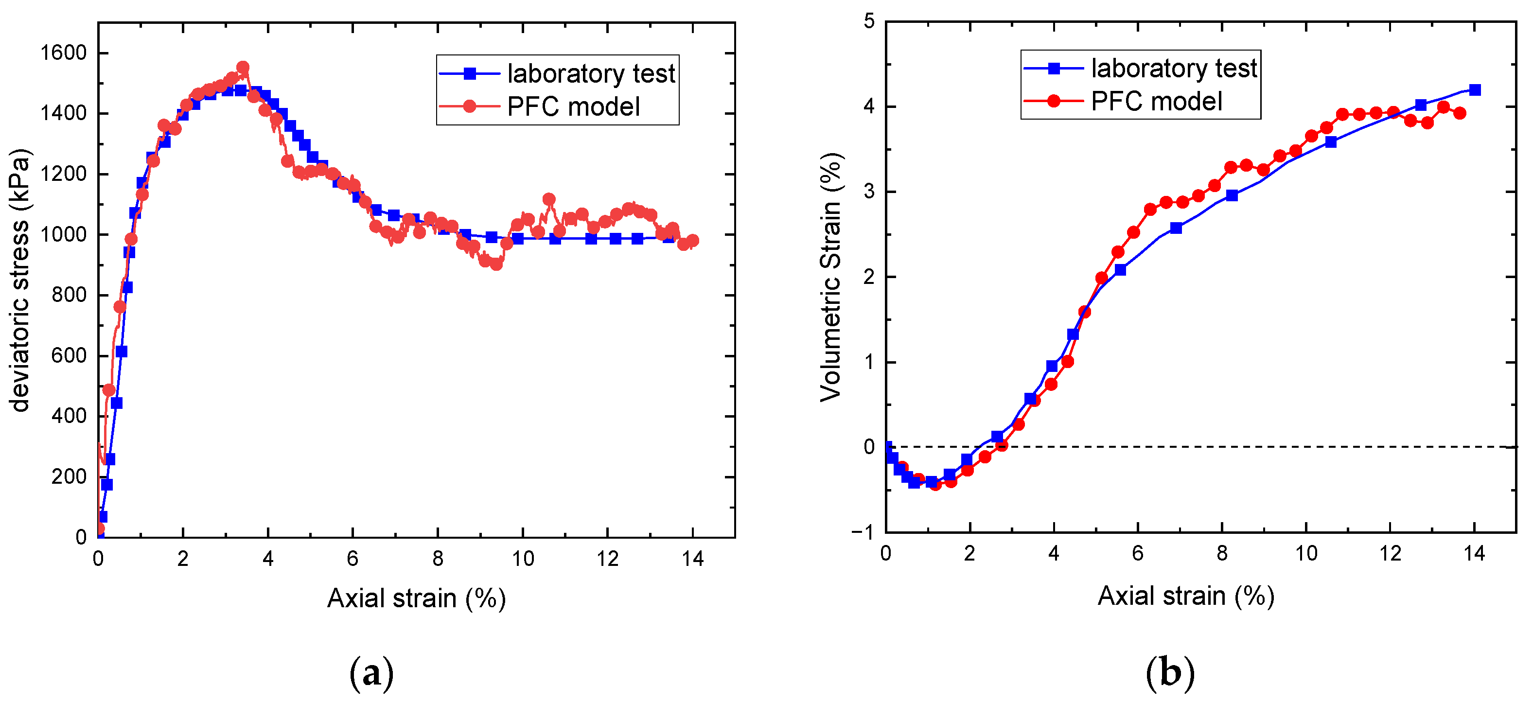
2.3. Microscopic Parameter Calibration

A finer calibration of $k_{\mathrm{n}}$, $\mu$, and $k_{\mathrm{s}}$ was implemented by considering the following three conditions.

• A slight increase in $\mu$ was implemented if the peak strength of the model was lower than that of the laboratory test, and vice versa.
• A slight increase in $\mu$ was implemented if the residual strength of the model was lower than that of the laboratory test, and vice versa.
• A slight increase in $k_{\mathrm{s}}$ was implemented if the initial slope of the stress–strain curve was lower than that of the laboratory test, and vice versa.

Based on the above methodology, we implemented a series of tests and finally took the microscopic parameters in

Table 1. Calibrated microscopic parameters.

	Density (kg/m3)	Stiffness (N/m)		Bonding Strength (N/m)		Friction Coefficient
		Normal	Tangential	Normal	Tangential
sand	2600	1.0 × 108	0.5 × 108	0	0	0.4
boundary	1000	5.0 × 107	5.0 × 107	1 × 1030	1 × 1030	0.0

. These parameters resulted in the stress–strain relationship in Figure 3. The initial porosity of the 2D model was 0.16, measured by the area of particles and the area of the specimen. The laboratory test was implemented using sands with particle sizes around 0.20–0.30 mm. It can be seen that good consistency is achieved. During the biaxial compression process of the specimen, the volumetric strain of the specimen first undergoes a compression stage. Then, shear dilation occurred, and volumetric strain increased. This is because when the stress is applied, the closely packed particles tend to move over each other. To accommodate this movement, the particles separate slightly and lead to an increase in volumetric strain. It should be mentioned that the porosity (and void ratio) depends largely on fine content because the fine particles occupy the void spaces between the coarse particles [23]. In this study, only the sand with one specific particle distribution was considered.

3. The Observation of the Size Effect

Then, the deformation and shear band of different-sized specimens were analyzed.

3.1. Models in Different Sizes

Before detailed tests, the DEM simulation was first compared with the electronic scan results by Mühlhaus and Vardoulakis [33] (Figure 4). Based on the DEM result, a rough estimation of the shear band is marked by blue lines. Accordingly, lines at the same position on the electronic scan are plotted. It can be seen that in both figures, the porosity inside the shear band significantly increases. The inclination angle and width obtained from DEM modeling are in good agreement with the electronic scan results. Therefore, the DEM modeling is believed to be capable of revealing the shear bands in actual sand.

Then, four specimens were generated under the same settings (particle size distribution, initial porosity, and microscopic parameters) except for the specimen sizes. These specimens were marked by S, M, L, and XL, respectively. The detailed specimen sizes are listed in

Table 2. The specimens in different sizes.

Specimens	$\mathit{H}$ (mm)	$\mathit{W}$ (mm)	$\mathit{W}/\overline{\mathit{R}}$	Particle Number
S	40	20	171	16,397
M	60	30	257	36,316
L	80	40	342	64,073
XL	100	50	482	99,577

Note: $H$ is specimen height, $W$ is specimen width, and $\overline{R}$ is the average radius of particles.

. Biaxial tests were implemented at isotropic confining stresses of 100 kPa, 300 kPa, 500 kPa, 700 kPa, and 900 kPa, respectively.

3.2. Size Effect in the Strain–Stress Curve

The strain–stress relationships at different isotropic confining stresses are plotted in Figure 5. It is observed that there are clear size effects after the peak strength point.

• The peak strengths of different-sized specimens were very close. As long as the deviatoric stress was less than the peak value, the stress–strain curves for different-sized specimens were very close. This indicates that the size effect was not obvious at the initial stage of the deformation.
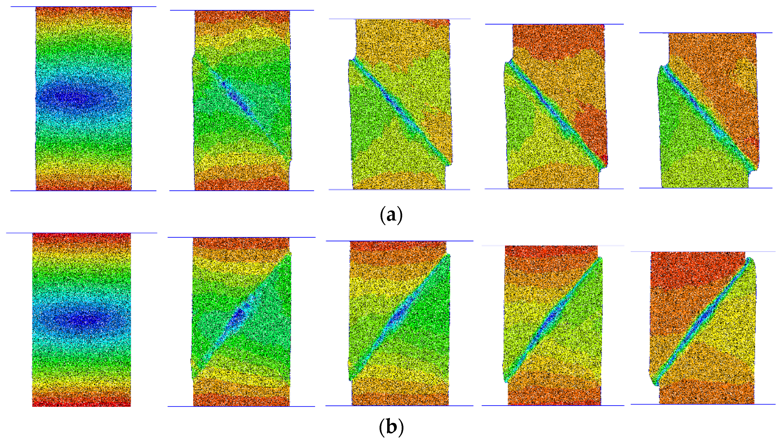
• A clear difference in the strain–stress curve was observed after the peak strength. Specifically, as the specimen size increased, the residual strength decreased. Such a size effect diminished as isotropic confining stress increased, and was evident in both biaxial compressive and biaxial tensile tests.

Based on the above finding, it is believed that, as the axial strain gradually increases, a transition from an internally stable state to an unstable state occurs at the peak strength point. Because strain concentrates within the narrow shear band, the deformation of the specimen became non-uniform. This might explain why different-sized specimens led to different stress–strain curves.

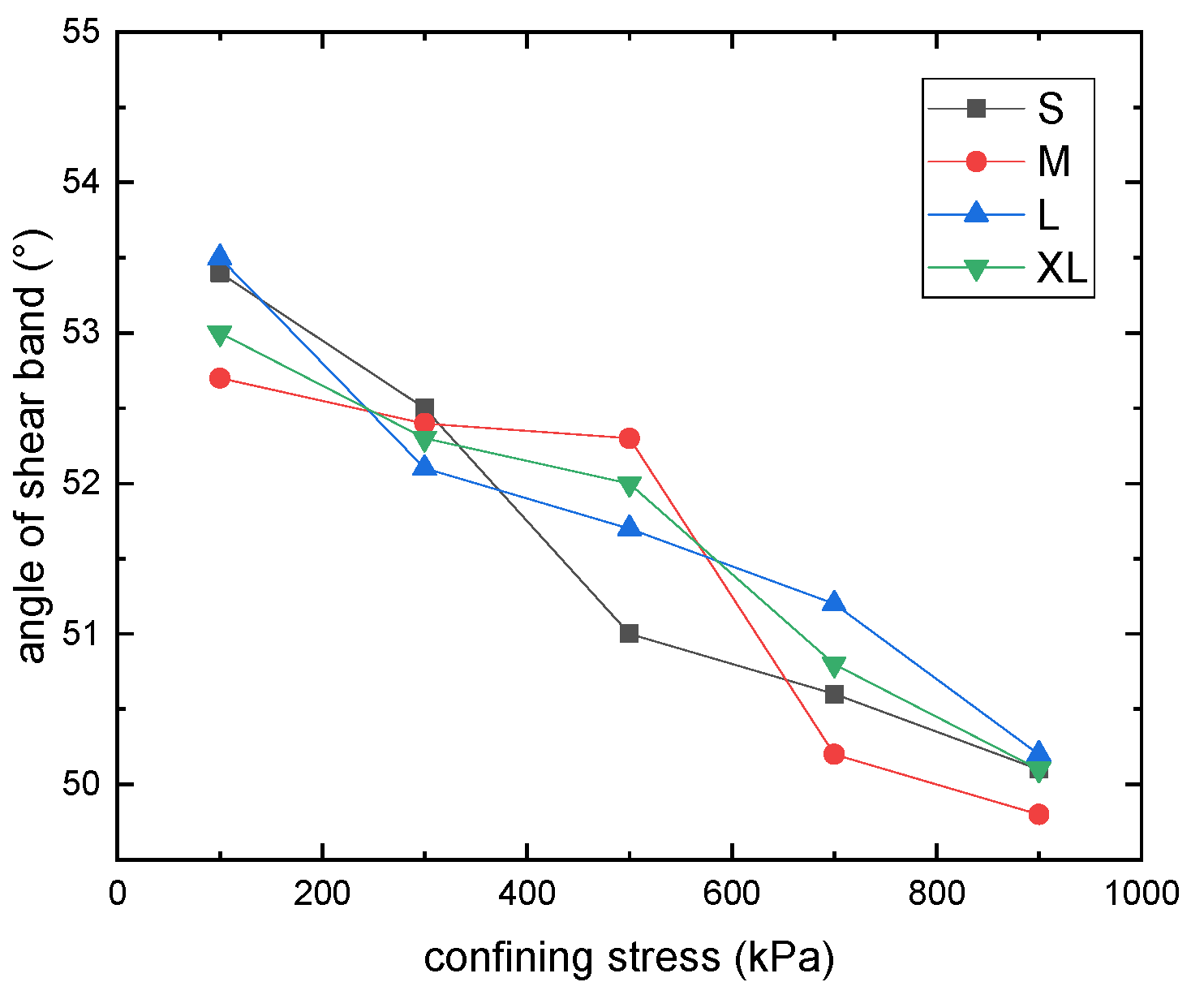
3.3. Less Size Effect in the Angle of Shear Bands

Less size effect was found on the angle of shear bands. The angles of different shear bands were mainly between 50 and 54°. As the isotropic confining stress increased, the angle of the shear band decreased to some extent (Figure 6).

There are three main theories about the angle of shear bands: Mohr–Coulomb theory, Roscoe theory, and Arthur theory [6,7,34]

$$\begin{array}{ll}\theta =\frac{\pi }{4}+\frac{\phi }{2}& \left(\text{Mohr-Coulomb}\right)\\ \theta =\frac{\pi }{4}+\frac{\psi }{2}& \left(\mathrm{Roscoe}\right)\\ \theta =\frac{\pi }{4}+\frac{\phi }{4}+\frac{\psi }{4}& \left(\mathrm{Arthus}\right)\end{array}$$

(4)

where φ is the friction angle, and ψ is the dilation angle obtained by

$$\sin \psi =\frac{\frac{\mathrm{d}{\epsilon }_v}{\mathrm{d}{\epsilon }_1}}{\frac{\mathrm{d}{\epsilon }_v}{\mathrm{d}{\epsilon }_1}-2}$$

(5)

where $\mathrm{d}{\epsilon }_v/\mathrm{d}{\epsilon }_1$ was calculated from the deformation inside the shear band.

It was calculated that $\psi =14.96°$; hence, the estimations of the Mohr–Coulomb, the Roscoe, and the Arthur formulas were 57.15°, 52.48°, and 54.8°, respectively. Our results were more consistent with the Roscoe type. Meanwhile, the size of the specimen had less impact on the angle of the shear band, because different-sized specimens led to similar results.

4. Explanations of the Size Effect

In Section 3, it is observed that as the specimen size increases, the peak strength and the angle of the shear band remain the same, while the residual strength decreases. Here, possible explanations are investigated.

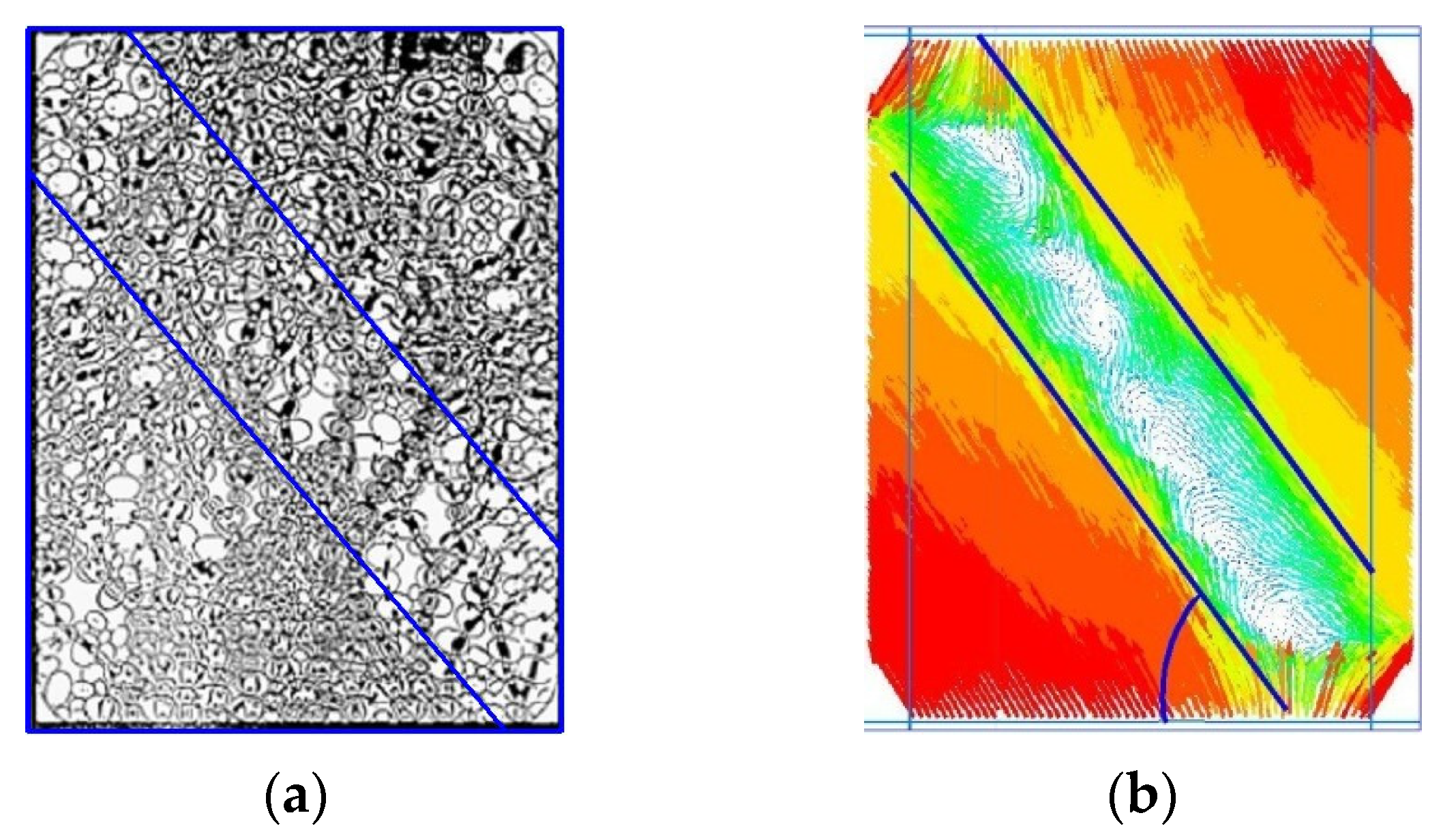
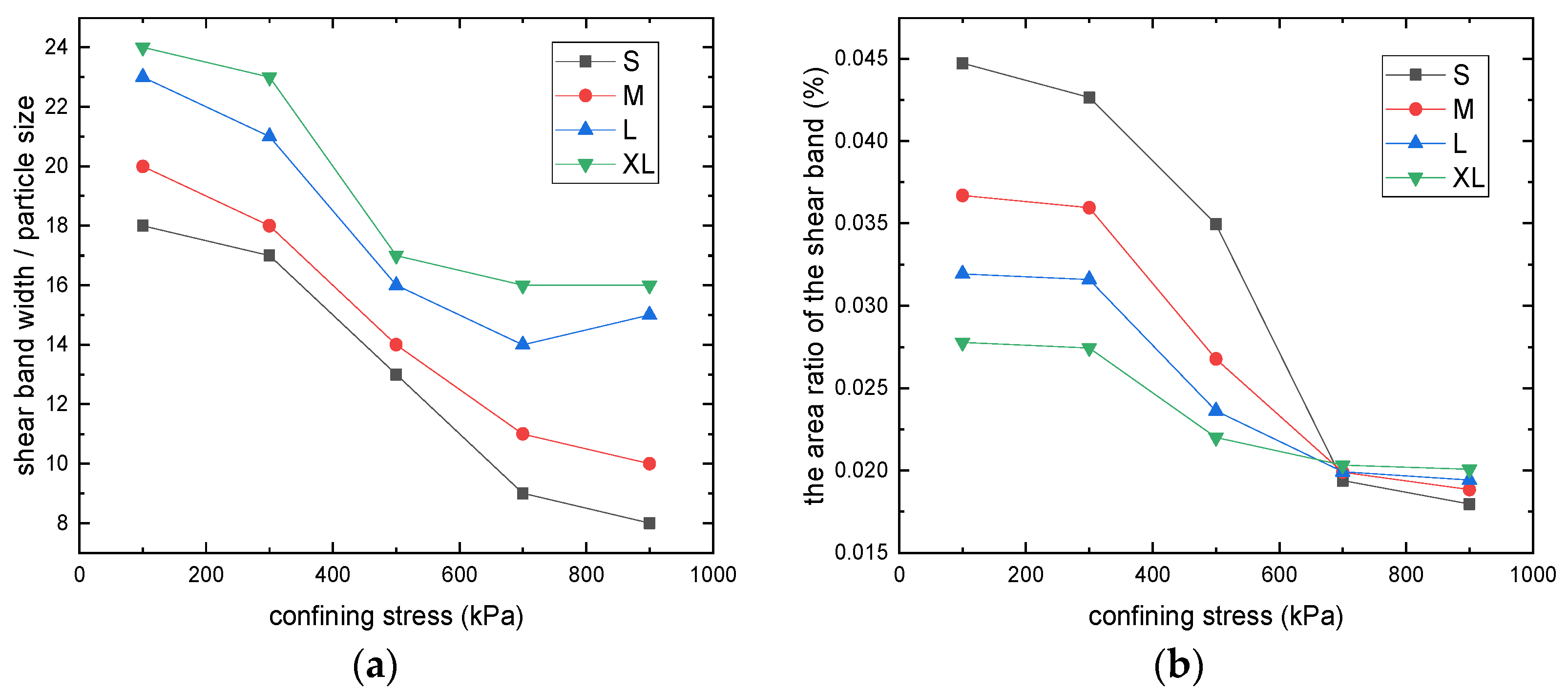
4.1. Explanations Based on the Characteristics of the Shear Band

During the test, it was observed that deformation was concentrated at shear bands, as plotted in Figure 7. It is noted that as the specimen size increased, the width of the basic shear band roughly remained unchanged. Accordingly, the proportion of the shear band decreased with the specimen size. That is to say, a larger specimen is more likely to fail because of a narrower shear band.

For a quantitative evaluation, the proportion of the shear band area (i.e., the ratio of the shear band to the initial specimen) against different isotropic confining stresses is plotted in Figure 8. The results show that:

• The area ratio gradually decreases as specimen size increases, although the width of the shear band increases with the specimen size.
• The degree of the decrease is related to the level of isotropic confining stress. At a higher isotropic confining stress level, the proportion of the shear band area of specimens tends to be the same. In detail, it can be seen that the width of the shear band is about 8–24 times the particle size, and as the isotropic confining stress increases, the width of the shear band gradually decreases and eventually stabilizes at a certain level.

The evolution of the shear band is also investigated. The evolutions of the displacement field of the smallest specimen (S) and the largest specimen (XL) are plotted in Figure 9. It is seen that as the shear band was generated, a relatively loose core area with high porosity formed at the center of the specimen. As the axial strain continued to increase, the shear band gradually developed towards both sides, the core area gradually disappeared, and the deformation became more concentrated in a narrow band area. Finally, stable shear bands were observed. The angles of the shear band of the two specimens were basically the same. The development of the shear band resulted in a sliding surface, and the particle structure of the soil near the sliding surface rapidly arranged and changed.

As to the influence of the isotropic confining stress, both the cross-type and the single-type shear bands can be observed in Figure 7 (this is also seen in, e.g., Alshibli and Sture [6]). One important finding is that the specimen tends to give cross-type shear bands at a low isotropic confining stress level. This could be a possible reason that the size effect is influenced by the magnitude of isotropic confining stress.

The influence of isotropic confining stress on the form of shear bands is analyzed thereby. During the shearing process, the specimen was first compressed and compacted. The soil near the loading plate gradually formed a rigid core. For a lower-level isotropic confining stress, the lateral isotropic confining stress cannot fully limit the deformation of the soil on both sides. The core area compressed the soil on both sides, causing the soil on both sides to detach from the core area. For a higher isotropic confining stress, the soil on both sides tightly adhered to the wedge-shaped rigid core area, limiting lateral deformation and increasing soil strength. As the shear process progressed, the internal soil of the specimen reached the ultimate stress state, and the upper and lower parts of the specimen experienced relative horizontal displacement. Subsequently, relative sliding occurred along the weak failure surface with a certain angle, resulting in a single-type shear band.

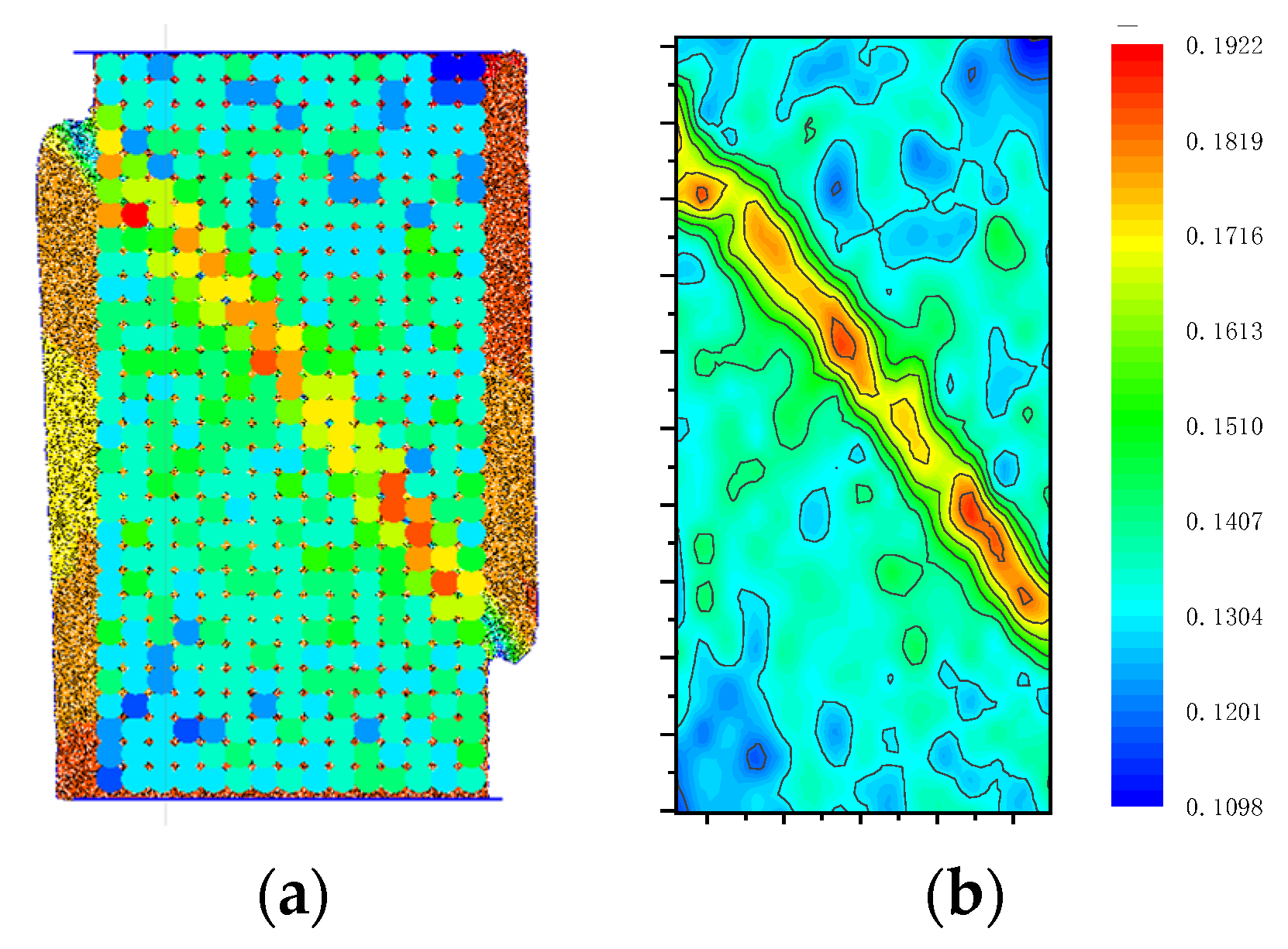
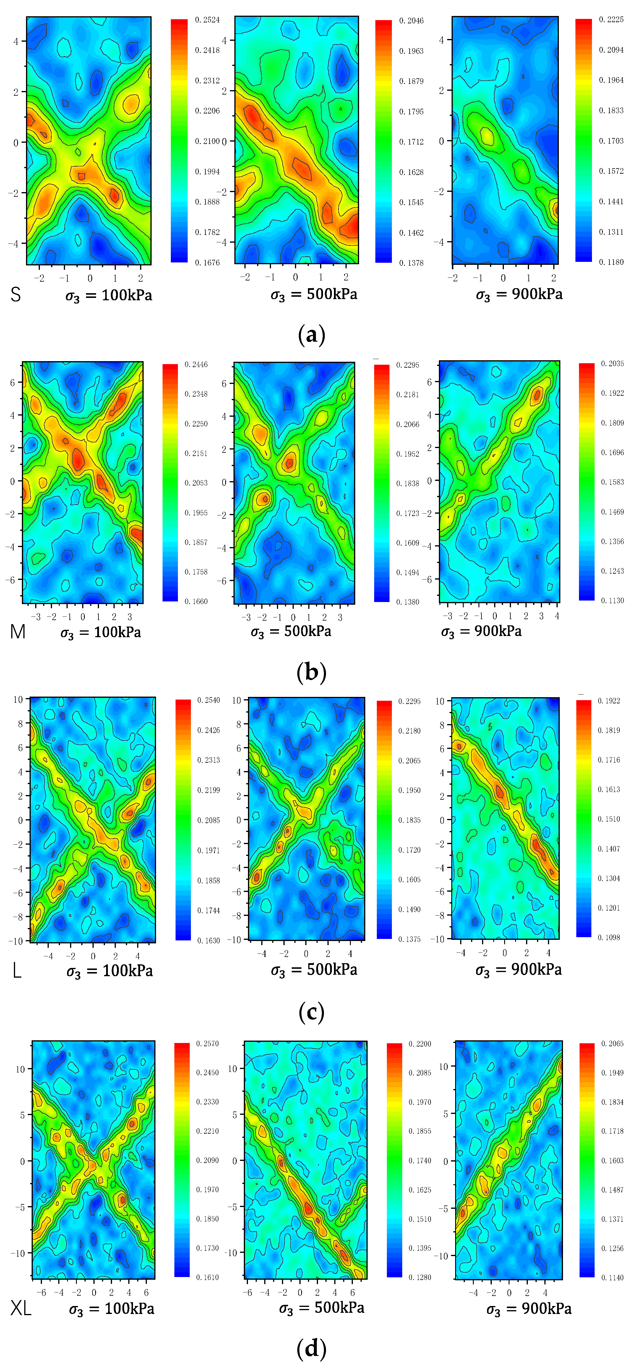
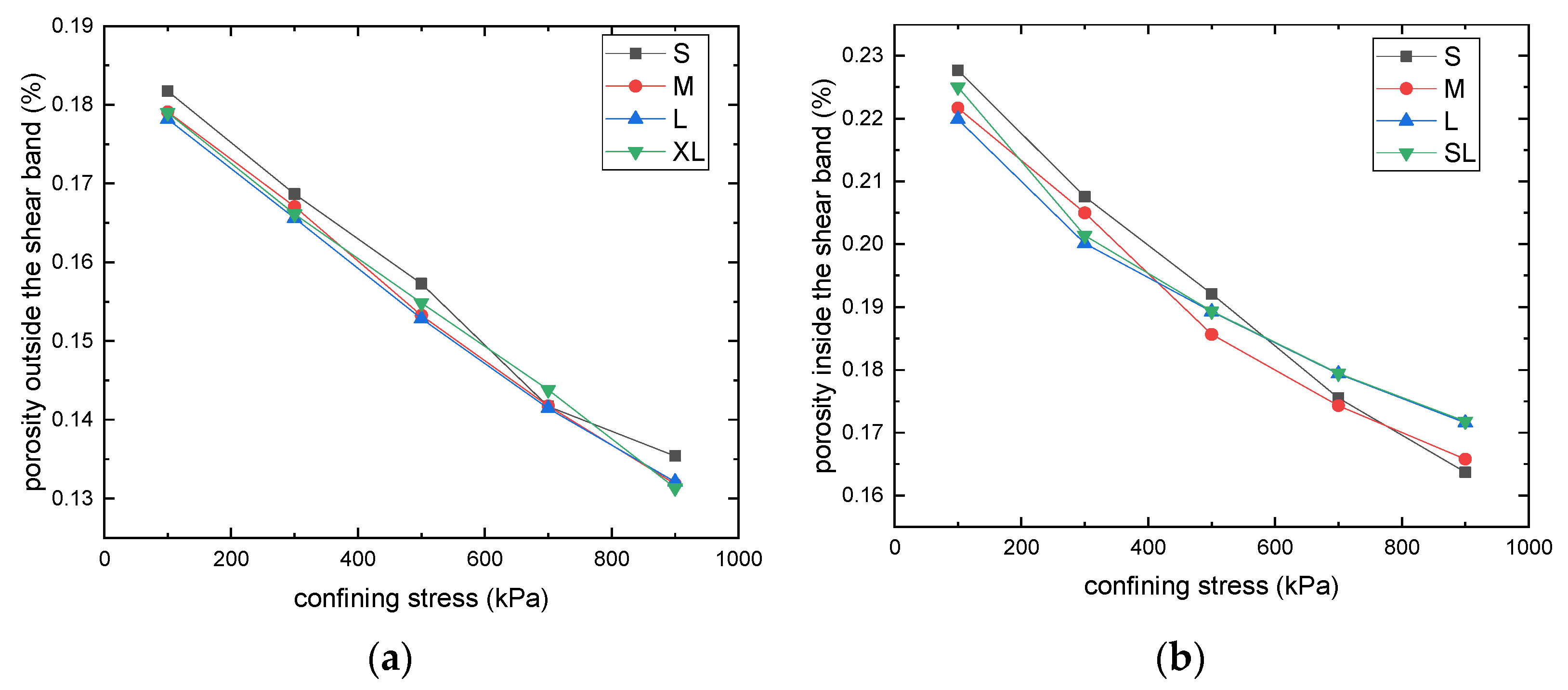
4.2. Porosity Inside and Outside the Shear Band

The formation of shear bands is the result of strain localization. To accurately determine the porosity inside and outside the shear band area, measuring circles were placed inside specimens (Figure 10), and the porosity was measured and plotted on a contour map. Thereby, the average porosities inside the shear band and outside the shear band were compared.

Through the above approach, we obtained the contours of porosity for different isotropic confining stresses at the same axial strain of 10% (Figure 11). The resulting shear bands included both single-type and cross-type. It was seen that the internal porosity of the shear band is relatively high, while the external porosity of the shear band is relatively small. For a lower-level isotropic confining stress, the proportion of shear band area in small specimens is significantly larger than that in large-sized specimens.

Together with the development of the deviatoric stress, the evolutions of the porosity inside and outside the shear band are plotted in Figure 12. It is noted that no matter whether inside or outside the shear band, there was a tendency for the porosity to increase first and then decrease. The transition point is about the peak strength point. Such a phenomenon is consistent with the size effect in Section 3. The porosity inside the shear band was finally stabilized, indicating that the critical state was reached.

To explore the size effect further, the relationship between the porosity and isotropic confining stress is plotted in Figure 13, where the porosity inside and outside the shear band area is considered separately. The porosity both inside and outside the shear band decreased with increasing isotropic confining stress. The porosity inside and outside the shear band is consistent under various isotropic confining stress conditions; therefore, the size effect of the specimen deformation characteristics is mainly caused by the difference in the proportion of the shear band area.

5. Conclusions and Prospects

In the context of soil mechanics, the shear band is an important concept, as it helps explain the behavior of granular materials under various loading conditions and the failure of slopes, dams, etc. Although the shear band is a narrow region, it is responsible for the overall macroscopic behavior at the failure. In this study, the shear band characteristics and in particular the size effect are mainly focused on. The major conclusions are as follows.

• As specimen size increases, the residual strength of the specimen decreases. A clear size effect was observed in the stress–strain relationship after the peak strength point. Such a size effect decreased as isotropic confining stress increased, and it was observed for both biaxial compressive and biaxial tensile tests.
• The increase in the specimen size has less impact on the angle of the shear band. Compared with Mohr–Coulomb’s theory and Roscoe’s theory, Arthur’s theory gave the best estimation of the angle of the shear band for the dense sand.
• A possible explanation of the size effect was found by instigating the development of displacement and porosity within the shear band. Although the width of the shear band increased to some extent with the size of the specimen, the ratio of the shear band in the whole specimen decreased. Accordingly, the concentration of strain became more obvious for a large specimen.
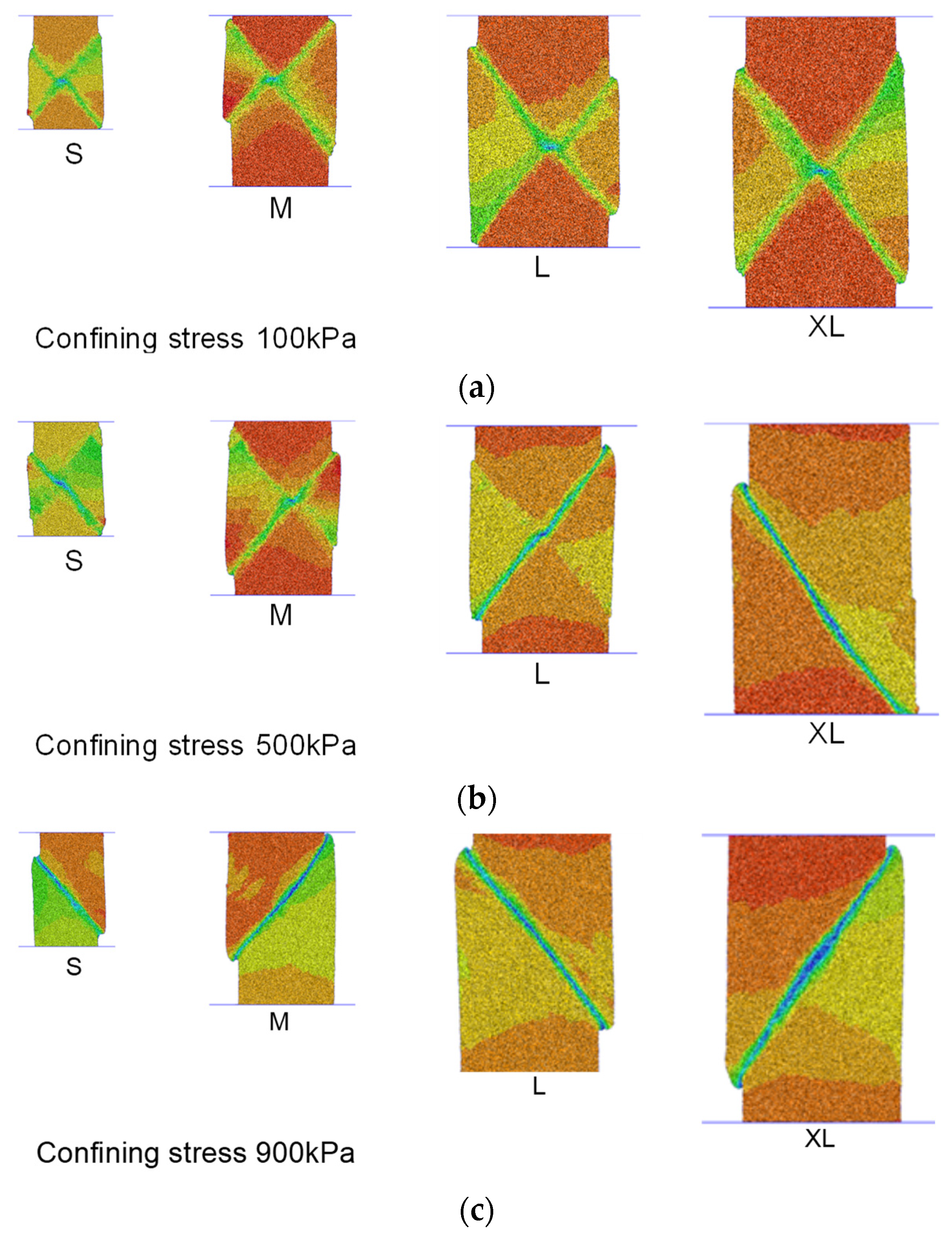
• The size effect reduces as the isotropic confining stress increases. Meanwhile, the specimen tends to give a cross-type shear band at a low isotropic confining stress level. The latter could be a possible reason that the size effect is influenced by the magnitude of isotropic confining stress.

Currently, only one particle distribution was considered throughout this paper. Further study should consider more soils for general conclusions.

References

1. Gudehus, G.; Nübel, K. Evolution of shear bands in sand. Geotechnique 2004, 54, 187–201. [Google Scholar] [CrossRef]
2. Rechenmacher, A.L. Grain-scale processes governing shear band initiation and evolution in sands. J. Mech. Phys. Solids 2006, 54, 22–45. [Google Scholar] [CrossRef]
3. Roscoe, K.H. The influence of strains in soil mechanics. Geotechnique 1970, 20, 129–170. [Google Scholar] [CrossRef]
4. Rattez, H.; Shi, Y.; Sac-Morane, A.; Klaeyle, T.; Mielniczuk, B.; Veveakis, M. Effect of grain size distribution on the shear band thickness evolution in sand. Géotechnique 2022, 72, 350–363. [Google Scholar] [CrossRef]
5. Silva, I.N.; Indraratna, B.; Nguyen, T.T.; Rujikiatkamjorn, C. The influence of soil fabric on the monotonic and cyclic shear behaviour of consolidated and compacted specimens. Can. Geotech. J. 2024; epub ahead of print. [Google Scholar]
6. Alshibli, K.A.; Sture, S. Shear band formation in plane strain experiments of sand. J. Geotech. Geoenviron. Eng. 2000, 126, 495–503. [Google Scholar] [CrossRef]
7. Han, C.; Drescher, A. Shear bands in biaxial tests on dry coarse sand. Soils Found. 1993, 33, 118–132. [Google Scholar] [CrossRef]
8. Viggiani, G.; Küntz, M.; Desrues, J. An experimental investigation of the relationships between grain size distribution and shear banding in sand. Contin. Discontin. Model. Cohesive-Frict. Mater. 2001, 568, 111–127. [Google Scholar]
9. Wang, Q.; Lade, P.V. Shear banding in true triaxial tests and its effect on failure in sand. J. Eng. Mech. 2001, 127, 754–761. [Google Scholar] [CrossRef]
10. Gu, X.; Huang, M.; Qian, J. Discrete element modeling of shear band in granular materials. Theor. Appl. Fract. Mech. 2014, 72, 37–49. [Google Scholar] [CrossRef]
11. Wiebicke, M.; Andò, E.; Viggiani, G.; Herle, I. Measuring the evolution of contact fabric in shear bands with X-ray tomography. Acta Geotech. 2020, 15, 79–93. [Google Scholar] [CrossRef]
12. Ramakrishnan, N.; Okada, H.; Atluri, S. On shear band formation: II. Simulation using finite element method. Int. J. Plast. 1994, 10, 521–534. [Google Scholar] [CrossRef]
13. Molinari, J.F.; Ortiz, M. Three-dimensional adaptive meshing by subdivision and edge-collapse in finite-deformation dynamic-plasticity problems with application to adiabatic shear banding. Int. J. Numer. Methods Eng. 2002, 53, 1101–1126. [Google Scholar] [CrossRef]
14. Baxevanis, T.H.; Katsaounis, T.; Tzavaras, A. Adaptive finite element computations of shear band formation. Math. Models Methods Appl. Sci. 2010, 20, 423–448. [Google Scholar] [CrossRef]
15. Daneshyar, A.; Mohammadi, S. Strong tangential discontinuity modeling of shear bands using the extended finite element method. Comput. Mech. 2013, 52, 1023–1038. [Google Scholar] [CrossRef]
16. Zhang, Z.H.; Zhang, G.D.; Li, X.L.; Xu, Z.H. The shear dilation and shear band of coarse grained soil based on discrete element method. Appl. Mech. Mater. 2015, 744, 679–685. [Google Scholar] [CrossRef]
17. Tang, H.; Zhang, X.; Ji, S. Discrete element analysis for shear band modes of granular materials in triaxial tests. Part. Sci. Technol. 2017, 35, 277–290. [Google Scholar] [CrossRef]
18. Yang, Y.; Tian, Y.; Yang, R.; Zhang, C.; Wang, L. Assessment of shear band evolution using discrete element modelling. Eng. Comput. 2024, 41, 183–201. [Google Scholar] [CrossRef]
19. Zienkiewicz, O.C.; Taylor, R.L.; Fox, D.D. The Finite Element Method for Solid and Structural Mechanics, 7th ed.; Elsevier: Singapore, 2015. [Google Scholar]
20. Evans, T.M.; Frost, J.D. Multiscale investigation of shear bands in sand: Physical and numerical experiments. Int. J. Numer. Anal. Methods Geomech. 2010, 34, 1634–1650. [Google Scholar] [CrossRef]
21. Khoei, A.; Tabarraie, A.; Gharehbaghi, S. H-adaptive mesh refinement for shear band localization in elasto-plasticity Cosserat continuum. Commun. Nonlinear Sci. Numer. Simul. 2005, 10, 253–286. [Google Scholar] [CrossRef]
22. Hutchinson, J.; Fleck, N. Strain gradient plasticity. Adv. Appl. Mech. 1997, 33, 295–361. [Google Scholar]
23. Haq, S.; Indraratna, B.; Nguyen, T.T.; Rujikiatkamjorn, C. Micromechanical Analysis of Internal Instability during Shearing. Int. J. Geomech. 2023, 23, 04023078. [Google Scholar] [CrossRef]
24. Bažant, Z.P.; Ožbolt, J.; Eligehausen, R. Fracture size effect: Review of evidence for concrete structures. J. Struct. Eng. 1994, 120, 2377–2398. [Google Scholar] [CrossRef]
25. Karihaloo, B.L.; Abdalla, H.; Xiao, Q. Size effect in concrete beams. Eng. Fract. Mech. 2003, 70, 979–993. [Google Scholar] [CrossRef]
26. Cundall, P.A.; Pierce, M.E.; Mas Ivars, D. Quantifying the size effect of rock mass strength. In Proceedings of the SHIRMS 2008: Proceedings of the First Southern Hemisphere International Rock Mechanics Symposium, Perth, Australia, 16–19 September 2008; pp. 3–15. [Google Scholar]
27. Yu, Q.; Zhu, W.; Ranjith, P.; Shao, S. Numerical simulation and interpretation of the grain size effect on rock strength. Geomech. Geophys. Geo-Energy Geo-Resour. 2018, 4, 157–173. [Google Scholar] [CrossRef]
28. Oda, M.; Kazama, H. Microstructure of shear bands and its relation to the mechanisms of dilatancy and failure of dense granular soils. Geotechnique 1998, 48, 465–481. [Google Scholar] [CrossRef]
29. Jiang, M.; Li, X. DEM simulation of the shear band of sands in biaxial tests. J. Shandong Univ. (Eng. Sci.) 2010, 40, 52–58. [Google Scholar]
30. Chen, Y.; Yu, Y.; She, Y. Method for determining mesoscopic parameters of sand in three-dimensional particle flow code numerical modeling. Chin. J. Geotech. Eng. 2013, 35, 88–93. [Google Scholar]
31. Luo, Y.; Gong, X.; Lian, F. Simulation of mechanical behaviors of granular materials by three-dimensional discrete element method based on particle flow code. Chin. J. Geotech. Eng. 2008, 30, 292–297. [Google Scholar]
32. Zhang, Q.; Wang, X.; Zhao, Y.; Liu, L.; Lin, X. Particle flow modelling of deformation and failure mechanism of soil-rock mixture under different loading modes of confining pressure. Chin. J. Geotech. Eng. 2018, 40, 2051–2060. [Google Scholar]
33. Mühlhaus, H.B.; Vardoulakis, I. The thickness of shear bands in granular materials. Geotechnique 1987, 37, 271–283. [Google Scholar] [CrossRef]
34. Das, B.M. Advanced Soil Mechanics; CRC Press: Boca Raton, FL, USA, 2019. [Google Scholar]
Figure 1. Traditional method vs. proposed method (take the traditional method first, then change to flexible boundaries to eliminate the influence of boundary conditions. Arrows represent the confining stress to be applied).
Applsci 14 04677 g001
Figure 2. Illustration of equivalent forces on particles of the flexible boundaries (1, 2, and 3 are three particles in the flexible boundaries).
Applsci 14 04677 g002
Figure 3. Comparisons of results obtained by triaxial tests and numerical simulations: (a) stress–strain relationship; (b) development of volumetric strain.
Applsci 14 04677 g003
Figure 4. Comparison of shear bands (specimen size 6 mm × 9 mm): (a) electronic scan results [33]; (b) the results obtained by DEM modeling (the shear band zone was estimated by the field of displacement magnitude).
Applsci 14 04677 g004
Figure 5. Stress–strain curves and development of volumetric strain of tests under different confining stress: (a) 100 kPa; (b) 300 kPa; (c) 500 kPa; (d) 700 kPa; (e) 900 kPa.
Applsci 14 04677 g005aApplsci 14 04677 g005b
Figure 6. The influence of isotropic confining stress on the angle of the shear band.
Applsci 14 04677 g006
Figure 7. The specimen tends to give a cross-type shear band at a lower isotropic confining stress and a single-type shear band at a larger isotropic confining stress. (a) Confining stress 100 kPa; (b) confining stress 500 kPa; (c) confining stress 900 kPa.
Applsci 14 04677 g007
Figure 8. The statistical results of the width of shear bands. (a) The width of the shear band; (b) the area ratio of the shear band.
Applsci 14 04677 g008
Figure 9. The evolution process of the shear band at the isotropic confining stress of 900 kPa: (a) specimen S; (b) specimen XL.
Applsci 14 04677 g009
Figure 10. Measuring circles and the contour plot of porosity. (a) The original data in measuring circles; (b) the contour plot of the porosity.
Applsci 14 04677 g010
Figure 11. Contours of porosity: (a) specimen size: S; (b) specimen size: M; (c) specimen size: L; (d) specimen size: XL.
Applsci 14 04677 g011
Figure 12. The development of porosity during compression.
Applsci 14 04677 g012
Figure 13. The porosity at an axial strain of 10%: (a) the porosity outside the shear band; (b) the porosity inside the shear band.
Applsci 14 04677 g013