A New Order Tracking Method for Fault Diagnosis of Gearbox under Non-Stationary Working Conditions Based on In Situ Gravity Acceleration Decomposition

Abstract

Rotational speed measuring is important in order tracking under non-stational working conditions. However, sometimes, encoders or coded discs are not easy to mount due to the limited measurement environment. In this paper, a new in situ gravity acceleration decomposition method (GAD) is proposed for rotational speed estimation, and it is applied in the order tracking scene for fault diagnosis of a gearbox under non-stationary working conditions. In the proposed method, a MEMS accelerometer is locally embedded on the rotating shaft or disc in the tangential direction. The time-varying gravity acceleration component is sensed by the in situ accelerometer during the rotation of the shaft or disc. The GAD method is established to exploit the gravity acceleration component based on the linear-phase finite impulse response (FIR) filter and complete ensemble empirical mode decomposition with adaptive noise (CEEMDAN) methods. Then, the phase signal of time-varying gravity acceleration is derived for rotational speed estimations. A motor–shaft–disc experimental setup is established to verify the correctness and effectiveness of the proposed method in comparison to a mounted encoder. The results show that both the estimated average and instantaneous rotational speed agree well with the mounted encoder. Furthermore, both the proposed GAD method and the traditional vibration-based tacholess speed estimation methods are applied in the context of order tracking for fault diagnosis of a gearbox. The results demonstrate the superiority of the proposed method in the detection of tooth spalling faults under non-stationary working conditions.

1. Introduction

An accurate measurement of rotational speed is important in condition monitoring, fault diagnosis and torsional vibration analysis for rotating machinery, e.g., gearbox and rotor-bearing systems [1,2,3]. Many common fault diagnosis methods, such as time synchronous average (TSA) and order analysis (OA), all have high requirements for accurate rotational speed. Therefore, it is of great significance to measure the rotational speed stably and accurately [4,5].

At present, encoder, toothed or notched encoder discs are the most wildly used methods for rotational speed measurements. The underlying mechanism of the encoder-based approach is that as the shaft rotates, a tooth or notch in the encoder disc will generate a series of pulse signals, and the rotational speed can then be obtained by counting the number of pulses [6]. The measured instantaneous rotational speed through the encoder-based method has been successfully applied in fault diagnosis and condition monitoring of rotating machinery. For instance, Zhao et al. proposed a kurtosis-guided local polynomial differentiator to estimate the instantaneous angular speed (IAS) of rotating machines based on the encoder signal; the results demonstrated that the proposed method could not only detect fault signatures but also identify defective components of a planetary gearbox [7]. However, sometimes the kurtosis is sensitive to the impulsive noise component, which is not beneficial for the estimation. Shao et al. introduced a new concept of root mean square (RMS) value calculations using angle domain signals within small angular ranges; a new diagnosis algorithm based on the time pulses of an encoder was developed to overcome the difficulty of fault diagnosis for helical gears at low rotational speeds [8]. But the angular ranges are difficult to determine, it has a direct influence on the diagnosis accuracy. Chin et al. presented a novel approach to conducting the rephasing of encoder signals for absolute dynamic transmission error (DTE) measurements of a gearbox; not only deviations from an involute profile but also the average wear depths of all teeth were well estimated [9]. However, the DTE measurement usually needs a higher sampling rate of the encoder, especially in high rotational speed situations. Zhang et al. proposed a bearing fault diagnosis method based on angular domain resampling; the non-stationary vibration signals in the time domain are transformed into the angular domain [10]. Although encoders have many success cases in rotational speed measurements, DTE estimation and IAS estimation may not be suitable in some cases, e.g., high rotational speed situations, limited space, and in an oil-contaminated environment [11].

Therefore, many scholars have tried to estimate the rotational frequency from the vibration signal [12], current [13], vision [14], etc. Among these rotational frequency estimation methods, the vibration-based method is the most popular one because of its convenient installation and rich information [15]. The basic principle of the vibration-based estimation method is that when a machine rotates in varying speed conditions, the rotating frequency and characteristic frequency also vary synchronously. Hence, the rotating information can be obtained by extracting the instantaneous frequency or instantaneous phase [16]. For instance, Li et al. introduced a rolling element bearing defect detection method using the generalized synchrosqueezing transform guided by TF ridge enhancement to settle the problem of the time-varying shaft speed [17]. However, the TF ridge fusion strategy sometimes may degrade, especially when there is a big difference between TF ridge 1 and 2. Urbanek et al. investigated a two-step procedure for the estimation of the IAS with large fluctuations which combines the advantages of phase demodulation and TFR and overcomes the obstacles of the harmonic overlapping phenomenon [18]. However, this method imposes stringent requirements on the accuracy of the two resampling procedures involved. Wang et al. proposed a rotating speed isolation method to extract the instantaneous rotating frequency based on the short time–frequency transformation (STFT) spectrogram; the fault characteristic was detected in the angular domain for fault diagnosis [19]. Once the fault is weak, the speed estimation accuracy may be affected. Rodopoulos et al. presented a parametric method for the estimation of the instantaneous speed of rotating machines; the proposed approach exhibited good estimating behavior with computational simplicity [20]. However, the speed estimation may degrade when the harmonic components in the vibration signal are weak; further, some parameters should be determined before the estimation. Barrios et al. studied an algorithm to automatically estimate the rotational speed from the vibration generated by a gear pair; Singular Spectrum Decomposition was used for decomposing the vibration signal into the mono-component signals, and a non-quadratic phase coupling analysis was applied in order to detect the amplitude modulations [21]. Above all, many rotational frequency estimation methods have been proposed and applied for fault diagnosis of rotational machinery, but they still face the problem of large amount of computation and difficulty in improving the accuracy. Furthermore, the estimation accuracy is deeply dependent on the extraction of the harmonic components, the starting point selection of the IF, the resolution of the TFR, the noise components, etc.

In this paper, a new in situ time-varying gravity acceleration decomposition method (GAD) is proposed for rotational speed estimation, and it is applied in the order tracking scene for fault diagnosis of a gearbox under non-stationary working conditions. The core idea of the proposed method is to acquire the time-varying gravity acceleration component by using an in situ MEMS accelerometer during the rotation of the shaft or disc. The corresponding decoupling method GAD and instantaneous rotational phase calculation method are presented based on the linear-phase FIR filter design [22], CEEMDAN [23], Hilbert transformation [24], etc. The correctness and effectiveness of the proposed method are verified by a motor–shaft–disc experimental setup with a local in situ accelerometer. The results show that both the average and instantaneous rotational speed can be well estimated. Furthermore, the GAD method is applied in order tracking for fault diagnosis of a gearbox, and four kinds of vibration-based estimation methods are compared. The superiority of the proposed method in the detection of tooth spalling faults under non-stationary working conditions is verified. Overall, the main contributions of the proposed method can be outlined as follows:

(1)

A new gravity acceleration decomposition method is proposed for rotational speed estimation.

(2)

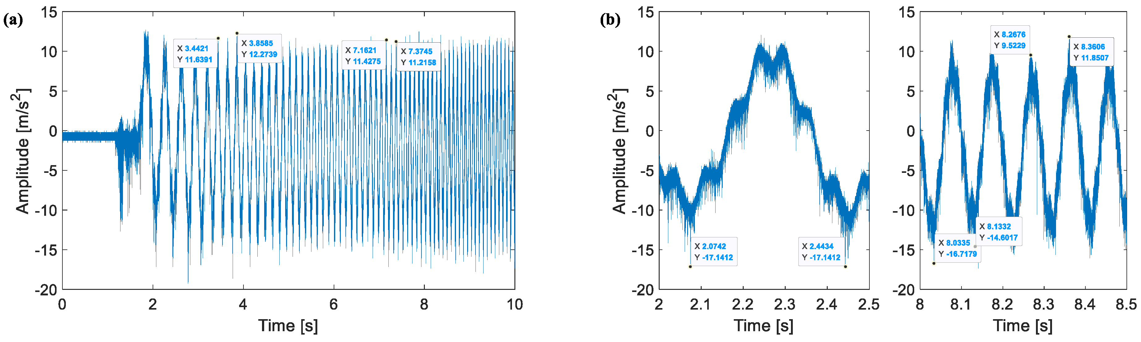
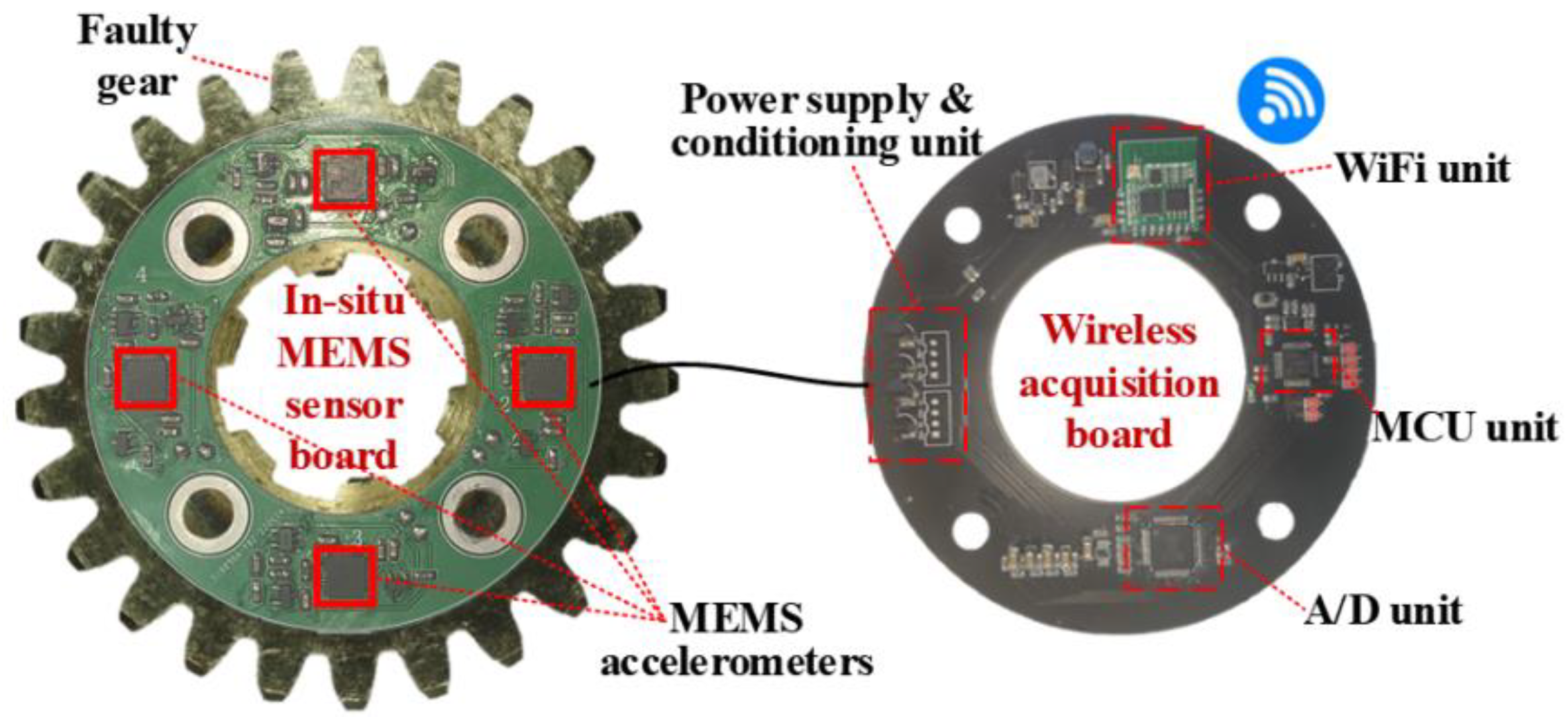
The time-varying gravity acceleration component is sensed by a tangentially mounted in situ MEMS accelerometer.

(3)

The proposed method yields better results in terms of order tracking than traditional vibration-based tacholess methods for fault diagnosis of a gearbox.

The rest of this paper is organized as follows. The underlying estimation principle of the instantaneous rotational speed based on the decoupled gravity acceleration component of the local in situ accelerometer is introduced in Section 2. The rotational speed estimation method based on CEEMDAN and Hilbert transformation is presented in Section 3. Then, the rotational speed estimation principle is verified in Section 4 based on a kinematic simulation of a rotor with the local in situ accelerometer. Then, six tests are conducted on an established motor–shaft–disc experimental setup in Section 5. Finally, the conclusions are drawn in Section 6.

2. Principle of Rotational Speed Estimation Based on In Situ MEMS Accelerometer

The estimation principle of the rotational speed based on gravity signals that are decoupled from an in situ accelerometer is shown in Figure 1. The core idea of the proposed method is to sense the variation in the gravity acceleration component of an in situ accelerometer as the disk rotates. Assuming that the in situ accelerometer is a bidirectional sensor, the sensitive directions are tangential and radial. Thus, the signal composition function in the two sensitive directions can be written as

$$S_T(t)=g•\cos \theta (t)+f_1\left[\ddot{\theta }(t),r\right]+f_2\left[\ddot{x}(t),\theta (t)\right]+f_3\left[\ddot{y}(t),\theta (t)\right]$$

(1)

$$S_V(t)=-g•\sin \theta (t)+{\omega }^2(t)•r+f_4\left[\ddot{x}(t),\theta (t)\right]+f_5\left[\ddot{y}(t),\theta (t)\right]$$

(2)

where g refers to the gravity acceleration. θ denotes the rotation angle. $\ddot{\theta }/\ddot{x}/\ddot{y}$ stand for the vibration acceleration in the torsional, horizontal and vertical directions, respectively. f₁[], f₂[] and f₃[] are the projection functions of $\ddot{\theta }/\ddot{x}/\ddot{y}$ in the tangential direction of the in situ accelerometer. r is the radius of the in situ accelerometer. ω means the rotating speed of the disc or shaft. f₄[] and f₅[] are the projection functions of $\ddot{x}/\ddot{y}$ in the radial direction of the in situ accelerometer.

Based on the observation of Equations (2) and (3), it can be found that the change process of gravity acceleration is included in both the tangential and radial directions. If gravity acceleration decoupling is achieved, the one-to-one correspondence relationship between θ and t can be obtained, and then, the rotational speed can be estimated based on the phase calculation of the acquired gravity acceleration component. However, it seems that the centrifugal acceleration component in the radial direction will be greatly affected by the instantaneous speed change and has a square relationship. It is expected that the accurate extraction of gravity acceleration will be disturbed in the case of variable speed in the radial direction of the in situ accelerometer. Therefore, this paper mainly focuses on an accurate extraction method for the tangential gravity acceleration component.

The key problem to be solved by this paper is to decouple the gravity acceleration component as accurately as possible, because the phase angle of the gravity acceleration component directly determines the estimation accuracy of the rotational speed.

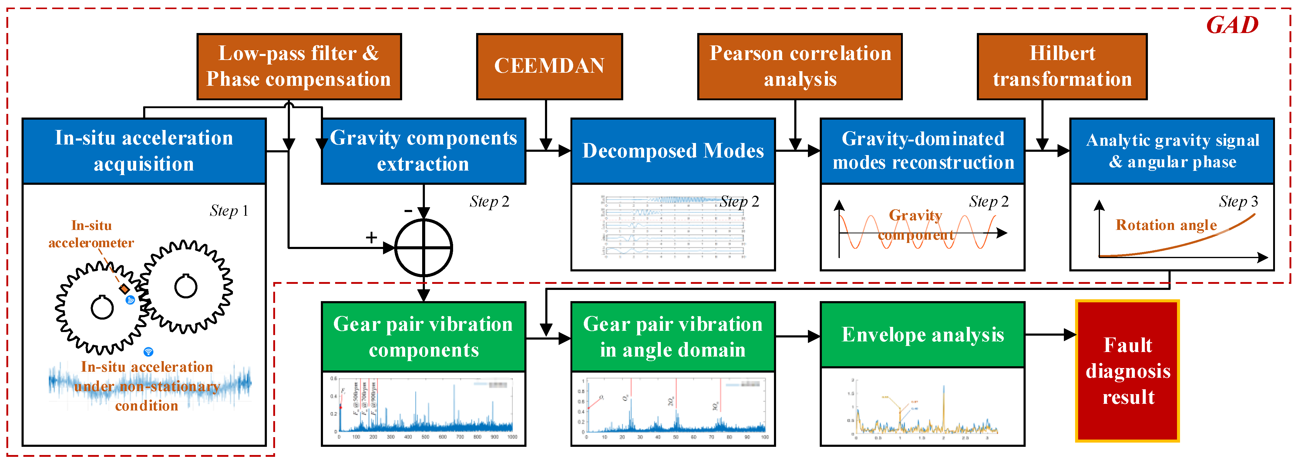
3. Order Tracking Based on the Proposed GAD Method

Figure 2 depicts the flowchart of the rotational speed estimation method based on GAD; there are mainly three steps in rotational speed estimation: data acquisition, decoupling of gravity acceleration and rotational speed evaluation. In step 1, a local in situ accelerometer is mounted on the rotating disc, and then, the signal is transferred from a wireless data transmission system; after that, the acquired signals are stored in the data acquisition system. In step 2, the GAD method is applied to derive the rotational phase for speed estimation. A low-pass filter is firstly adopted to suppress the high-frequency component of the torsional, horizontal and vertical vibration, and then, phase compensation is presented; after that, the mode decomposition method is used to improve the accuracy of the gravity acceleration component. In step 3, the rotational phase and speed are estimated based on Hilbert transformation and the phased unwrapping method. Furthermore, the estimated rotational speed is applied in the order tracking scene for fault diagnosis of a gearbox under non-stationary working conditions.

3.1. The Main Procedure of the GAD Method

As illustrated in Figure 2, the first step of the method is to mount the local in situ accelerometer. In this paper, the accelerometer is mounted tangentially to avoid the influence of centrifugal acceleration, i.e., in the circumferential direction or opposite to the rotation. Then, a linear-phase FIR filter and CEEMDAN are employed for time-varying gravity acceleration detection.

3.1.1. Linear-Phase Filter for Gravity Acceleration Component Detection

In order to detect the time-varying gravity acceleration component and ensure that the waveform does not change, a linear-phase FIR low-pass filter is designed based on the window function [25]. Firstly, the desired amplitude–frequency characteristics are given as

$$H_d(e^{j\omega })=\left\{\begin{array}{l}{e}^{-j\omega \alpha }\begin{array}{cc}& \left(\left|\omega \right|\le {\omega }_c\right)\end{array}\\ 0\begin{array}{ccc}& & \left({\omega }_c<\left|\omega \right|<\pi \right)\end{array}\end{array}\right.$$

(3)

where α denotes the time delay. Then, the desired unit pulse responses with a linear-phase can be obtained as

$$h_d(n)=\frac{1}{2\pi }{\displaystyle {\int }_{-\pi }^{\pi }{H}_d\left(e^{j\omega }\right)}{e}^{j\omega n}d\omega =\frac{1}{2\pi }{\displaystyle {\int }_{-\pi }^{\pi }{e}^{j\omega \alpha }}{e}^{j\omega n}d\omega =\frac{\sin \left[{\omega }_c(n-\alpha )\right]}{\pi (n-\alpha )}$$

(4)

$$\alpha =\frac{N-1}{2}$$

(5)

Then, the window function is adopted to cut off h_d to obtain a finite length sequence:

$$h(n)=h_d(n)w_N(n)\begin{array}{cc}& \left(n=0,1,\dots ,N-1\right)\end{array}$$

(6)

$$N=\frac{2\pi A}{\Delta \omega }$$

(7)

where w_N denotes the window function, N refers to the filter length, A means the constant related to the window function and Δω represents the transition band width between the passband and stopband.

The band containing the gravity acceleration component can be calculated based on the derived filter, as follows:

$$S_g(t)=h\ast Sig(t)$$

(8)

where Sig(t) represents the acquired vibration signal of the local in situ accelerometer. And it is known that there is a linear-phase delay after FIR filtering, so a phase compensation step is applied, in which the phase delay in the design filter is α, and the compensated signal is marked as S_gc.

3.1.2. Noise Suppression for Gravity Acceleration Component Based on CEEMDAN

Based on the proposed estimation principle illustrated in Section 2, it is known that the rotating phase of the gravity acceleration component has a significant influence on the instantaneous rotational speed accuracy. And the rotating phase is calculated from the acquired vibration signal. Therefore, it is important to improve the signal-to-noise ratio (SNR) of the decoupled gravity acceleration component, and the expected ultimate goal is to make the signal only contain a single component of gravity.

To achieve this goal, the CEEMDAN method is adopted for SNR improvement, which is an improved version based on EEMD proposed by Torres et al. in 2011 [23,26]. The CEEMDAN method is essentially a variation of the EEMD algorithm that provides an exact reconstruction of the original signal and better spectral separation of the modes, with a lower computational cost. However, there are also some disadvantages of the CEEMDAN method, i.e., a large computation cost, poor decomposition performance with large noises, etc. Hence, the CEEMDAN method is only used as an example to decompose the signal. Empirical wavelet transformation (EWT) [27] and the ICEEMDAN method [28] will also be used and compared in the decomposition of the vibration signal. Details of the procedure of noise suppression of the gravity acceleration component based on CEEMDAN are as follows:

• Step 1: First IMF detection from the gravity acceleration component S_gc[n].

Decompose the I realizations $S_{gc}[n]+{\epsilon }_0{w}^i[n]$, i = 1, 2, …, to obtain their first modes and compute their average:

$${\widetilde{IMF}}_1[n]=\frac{1}{I}{\displaystyle {\sum }_{i=1}^{I}IM{F}_1^i[n]}={\overline{IMF}}_1[n]$$

(9)

where wⁱ refers to white noise with N(0, 1).

• Step 2: First residue r₁[n] calculation.

Calculate the first residue as follows:

$$r_1[n]=S_{gc}[n]-{\widetilde{IMF}}_1[n].$$

(10)

• Step 3: Second IMF detection from residue r₁[n].

Decompose the realizations $r_1[n]+{\epsilon }_1{E}_1\left(w^i[n]\right)$ until you obtain their first EMD mode and define the second mode as follows:

$${\widetilde{IMF}}_2[n]=\frac{1}{I}{\displaystyle {\sum }_{i=1}^I{E}_1\left(r_1[n]+{\epsilon }_1{E}_1(w^i[n])\right)}$$

(11)

where E_j(•) is defined as an operator that produces the jth mode of a signal obtained by the EMD algorithm.

• Step 4: kth residue r_k[n] calculation.

Calculate the kth residue, k = 2, …, K, as follows:

$$r_k[n]=r_{(k-1)}[n]-{\widetilde{IMF}}_k[n].$$

(12)

• Step 5: (k + 1)th IMF detection.

Decompose the realizations $r_k[n]+{\epsilon }_k{E}_k\left(w^i[n]\right)$ until you obtain their first EMD mode and define the (k + 1)th mode as follows:

$${\widetilde{IMF}}_{(k+1)}[n]=\frac{1}{I}{\displaystyle {\sum }_{i=1}^I{E}_1\left(r_k[n]+{\epsilon }_k{E}_k(w^i[n])\right)}.$$

(13)

• Step 6: Repetition of step 4 and 5.

Go to step 4 for the next k until the obtained residue is no longer feasible to be decomposed.

Therefore, the gravity acceleration component S_gc[n] can be expressed as follows:

$$S_{gc}[n]={\displaystyle {\sum }_{k=1}^K{\widetilde{IMF}}_k+R[n]}$$

(14)

where R[n] represents the last residue. Then, the Pearson correlation coefficients [29] between each IMF and S_gc are calculated. It is expected that the IMF with the highest coefficient contains the most information about the gravity acceleration component due to low-pass filtering in Section 3.1.1. The calculation equation can be obtained as follows:

$$r_k=corr\left({\widetilde{IMF}}_k,S_{gc}\right)=\frac{{\displaystyle {\sum }_{n=1}^N\left[{\widetilde{IMF}}_k\left(n\right)-mean\left({\widetilde{IMF}}_k\right)\right]\left[S_{gc}\left(n\right)-mean\left(S_{gc}\right)\right]}}{\sqrt{{\displaystyle {\sum }_{n=1}^N{\left[{\widetilde{IMF}}_k\left(n\right)-mean\left({\widetilde{IMF}}_k\right)\right]}^2}}\sqrt{{\displaystyle {\sum }_{n=1}^N{\left[S_{gc}\left(n\right)-mean\left(S_{gc}\right)\right]}^2}}}.$$

(15)

Finally, the IMFs containing the gravity acceleration component will be selected for rotational speed estimation based on the Pearson relationship coefficient, which is obtained as follows:

$$S_{gc\_d}(t)=w_1•{\widetilde{IMF}}_1+w_2•{\widetilde{IMF}}_2+\dots +w_K•{\widetilde{IMF}}_K$$

(16)

$$w_k=\left\{\begin{array}{ll}1,& r_k>Thr\\ 0,& r_k\le Thr\end{array}\right.$$

(17)

where Thr is the selected threshold, which is set as the mean value of the relationship coefficients in this paper.

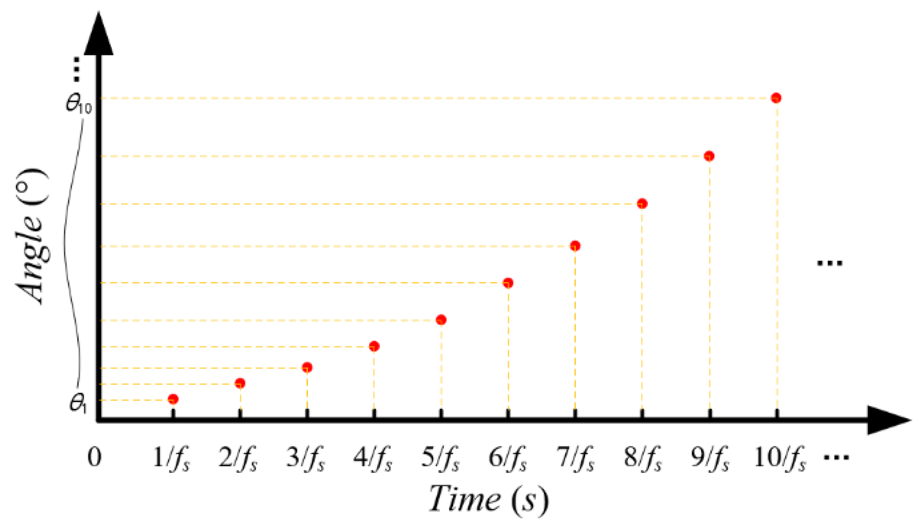
3.2. Rotational Speed Estimation and Order Tracking

In this section, the rotating phase of the gravity acceleration component is first calculated from its analytic signal based on Hilbert transformation. The analytic signal of the gravity acceleration component can be obtained as follows:

$${\overline{S}}_{gc\_d}(t)=S_{gc\_d}(t)+j{\widehat{S}}_{gc\_d}(t)=A(t)•e^{j\phi (t)}$$

(18)

$${\widehat{S}}_{gc\_d}(t)=H\left\{S_{gc\_d}(t)\right\}=S_{gc\_d}(t)\otimes \frac{1}{\pi t}={\displaystyle {\int }_{-\infty }^{+\infty }\frac{S_{gc\_d}(\tau )}{t-\tau }}d\tau$$

(19)

where ${\widehat{S}}_{gc\_d}(t)$ represents the signal after Hilbert transformation, and H{} means the Hilbert operator. ${\overline{S}}_{gc\_d}(t)$ denotes the obtained analytic signal. A(t) and φ(t) refer to the instantaneous amplitude and phase, which can be determined as follows [30]:

$$A(t)=\sqrt{S^2{ }_{gc\_d}(t)+{\widehat{S}}_{gc\_d}^2(t)}$$

(20)

$$\phi (t)=\arctan \frac{{\widehat{S}}_{gc\_d}(t)}{S_{gc\_d}(t)}$$

(21)

Based on Equations (22) and (23), the amplitude and phase of the gravity acceleration component are obtained. It can be seen from the estimation principle of rotational speed based on the decoupling of gravity variation that there is a one-to-one correspondence relationship between θ and t. Hence, the rotational angle and speed can be estimated further from φ(t). Since the instantaneous phase angle of φ(t) is in the interval [−π, π], the real-time rotation angle φ′(t) of the rotating disk or shaft relative to the initial moment can be obtained by using the unwrap method; thus, the obtained rotation angle is calculated, as illustrated in Figure 3.

Suppose the obtained phase angle is noted as θ = [θ₁, θ₂, …, θ_N]^T, the instantaneous rotational speed can be calculated as follows:

$$\omega (t)=\frac{\Delta \theta }{\Delta t}={\left[\Delta {\theta }_1•f_s\hspace{1em}\Delta {\theta }_2•f_s\hspace{1em}\Delta {\theta }_3•f_s\hspace{1em}\dots \hspace{1em}\Delta {\theta }_{N-1}•f_s\right]}^T$$

(22)

$$\Delta \theta ={\left[\Delta {\theta }_1\hspace{1em}\Delta {\theta }_2\hspace{1em}\Delta {\theta }_3\hspace{1em}\dots \hspace{1em}\Delta {\theta }_{n-1}\right]}^T={\left[{\theta }_2-{\theta }_1\hspace{1em}{\theta }_3-{\theta }_2\hspace{1em}{\theta }_4-{\theta }_3\hspace{1em}\dots \hspace{1em}{\theta }_N-{\theta }_{N-1}\right]}^T$$

(23)

$$\Delta t=\frac{1}{f_s}$$

(24)

Therefore, the rotational speed can be obtained based on the above methodology. It can be inferred that the resolution of the instantaneous angle in the proposed method is equal to the sampling frequency minus 1, which is much lower compared to the traditional encoder method.

4. Validation of the Rotational Speed Estimation Principle Using GAD

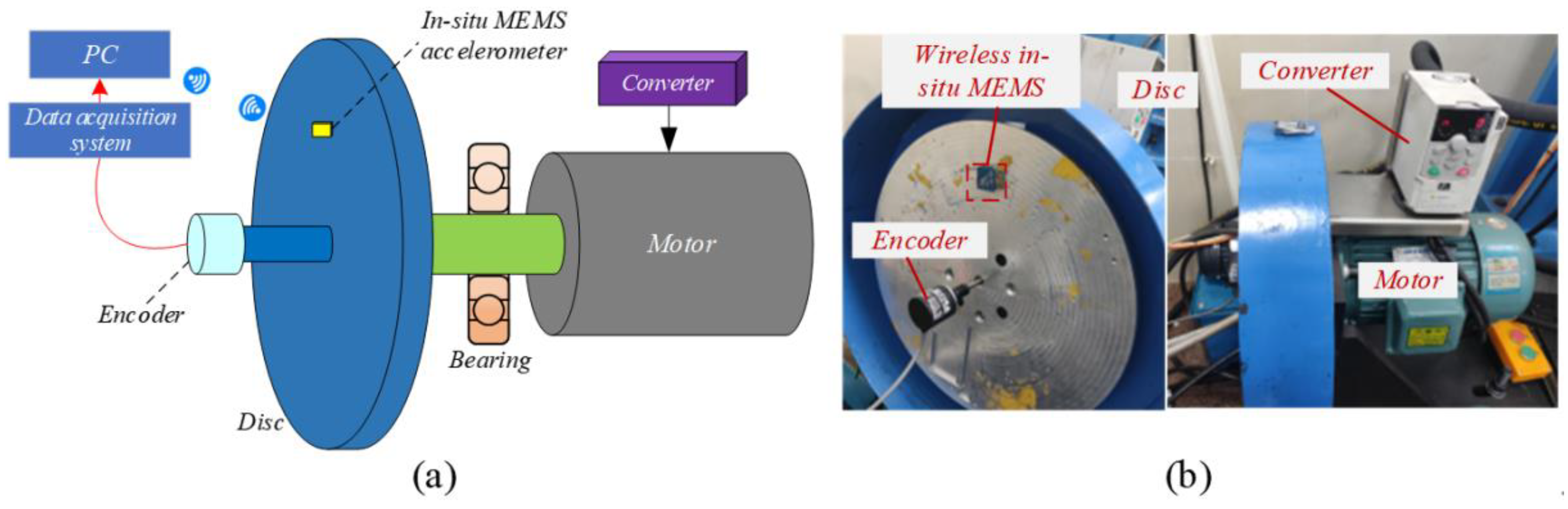
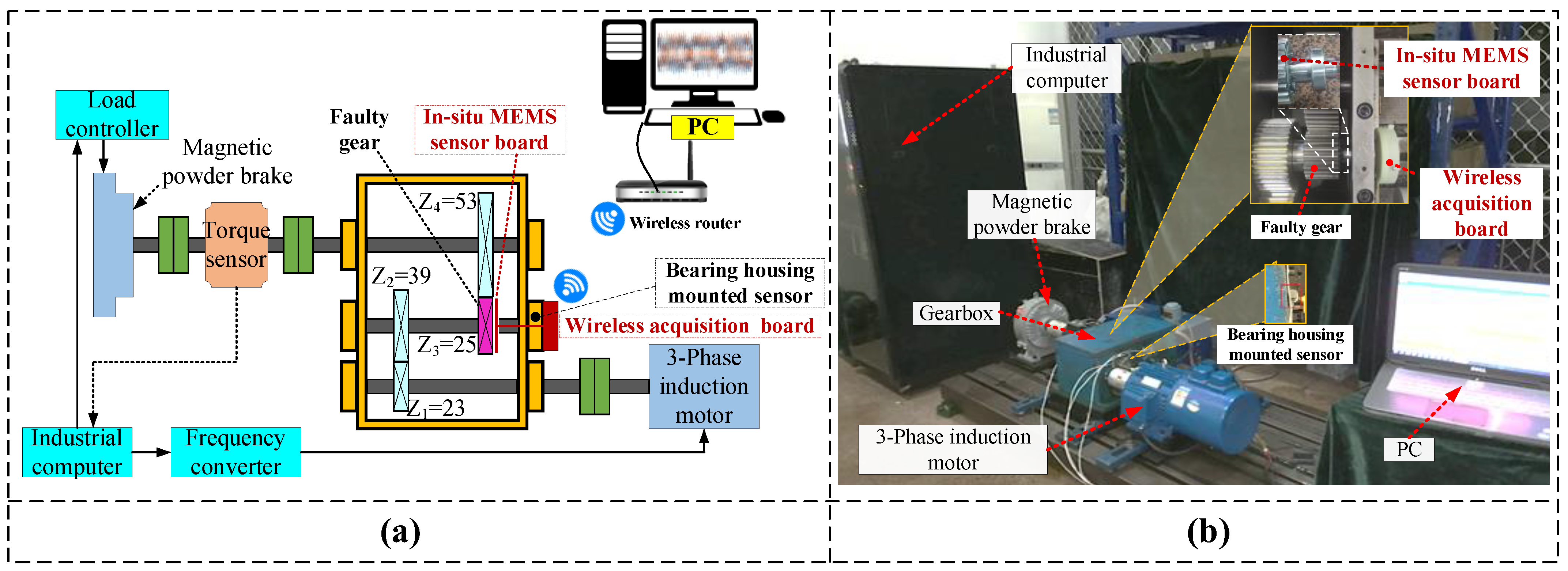
4.1. Experimental Setup

In order to verify the correctness and effectiveness of the proposed rotational speed estimation methodology, a motor–shaft–disc experimental setup is established. The setup mainly consists of a converter, a motor, a shaft, a disc, an encoder, etc., as illustrated in Figure 4. One in situ accelerometer is mounted on one end of the disc with the sensitive direction in the tangential direction. The mounting radius of the in situ accelerometer is approximately 20 mm. The selected accelerometer type is ADXL 1001 from Analog Devices in the Norwood, MA, USA, the measuring range is ±100 g and the sensitive value is 20 mv/g. In the experiment, an E6HZ-CWZ6C incremental encoder of OMRON from Kyoto, Japan is used to record the rotation angle in this paper, which is mounted on the end of the extension shaft. The encoder line is 360 P/R. The rotational speed is controlled by adjusting the converter.

Two tests are conducted based on the experimental setup: Test 01 involves the startup procedure, where the initial motor speed gradually increases from 0 r/min to 700 r/min within a time span ranging from 1.5 s to 9.9 s. Conversely, Test 02 focuses on the run-down procedure, during which the initial motor speed decreases from 620 r/min to 0 r/min within a time frame varying from 1.5 s to 8.5 s. The sampling frequency for the encoder is set as 204.8 kHz to guarantee the high-resolution accuracy of the encoder. And the sampling frequency for the in situ accelerometer is set as 4096 Hz. The sampling time length for both of the two measurement quantities is set as 10 s.

4.2. Speed Estimation Result Comparisons

(i) 

Test 01: startup working condition

The acquired acceleration signals from the tangential in situ accelerometer are illustrated in Figure 5. As can be seen from the original plot and the zoomed-in one, there exists a big sinusoidal periodic signal in the tangential accelerometer. The frequency of the sinusoidal periodic component grows over time, with a period similar to the rotational frequency of the disc. According to the signal composition analyzation in Equation (2), the sinusoidal periodic signal is caused by the time-varying gravity acceleration component. Hence, the rotational speed can be estimated by decoupling the gravity acceleration component from the acquired acceleration signal. However, it is obvious there are lots of noise components and interferences that need to be suppressed, as shown in Figure 5.

According to Equation (6) and the rated speed of the experimental setup, the cutoff frequency of the linear-phase low-pass filter is set as 100 Hz. The filtered local embedded acceleration signals are then obtained, as shown in Figure 6. Compared to the raw signals in Figure 5, lots of high-frequency components are suppressed based on the linear-phase low-pass filter, so the period of the gravity acceleration component becomes clearer. However, there are still lots of oscillations in both the low-speed range and high-speed range of the startup working condition, which is not conducive to the accurate estimation of the speed.

Then, the CEEMDAN method, ICEEMDAN method and EWT method are applied to the filtered local embedded acceleration signals to decouple the gravity acceleration components. The decomposed IMFs of the filtered acceleration signals based on the three methods are shown in Figure 7; there are 18, 15 and 15 decomposed IMFs in the three methods, the desired IMFs are highlighted by the red dashed frame in Figure 7. In the CEEMDAN method, it is found that the noise components are mainly decomposed into the first 8 IMFs, while the time-varying gravity components are decomposed into IMF 9 to 11, as shown in Figure 7a,b. But it seems there are still some high-frequency noises in IMF 9. In the ICEEMDAN method, the noise components are mainly located at the first 5 IMFs, while the time-varying gravity components are decomposed into IMF 6 to 10, and it seems the high-frequency noise suppression performance in IMF 6 to 10 is better, as shown in Figure 7c,d. In the EWT method, clearly decomposition of the vibration signal in the time and frequency dimension can be observed; the noise components are mainly located at the first 7 IMFs, while the time-varying gravity components are decomposed into IMF 8 to 14. The noise suppression performance based on the EWT method seems to be the best among the three methods, as depicted in Figure 7e,f.

The Pearson correlation coefficients between each IMF and the filtered local embedded acceleration signals are calculated for the three methods, as illustrated by the blue solid line in Figure 8. In this paper, the average value of all IMF correlation coefficients is used as the threshold to select sensitive IMFs, as shown by the red dotted line in Figure 8. It is found that the IMFs containing more time-varying gravity acceleration components are well selected based on the three methods.

The reconstructed gravity acceleration components under the Test 01 working condition based on the three methods are then obtained and compared, as shown in Figure 9. Most of the oscillations are suppressed in all of the three methods, especially in the high-speed range. And the magnitude of the reconstructed sinusoidal periodic component approximately equals the gravity in all of the three methods. During the initial startup phase, the presence of oscillations and noticeable differences among the CEEMDAN, ICEEMDAN and EWT methods are observed. Notably, the EWT method exhibits superior noise suppression performance. However, it is also observed that there are some reconstruction errors before the actual startup, which may be attributed to noise or interference. In conclusion, the utilization of the CEEMDAN, ICEEMDAN and EWT methods for decomposition and reconstruction reveals minimal differences among the three approaches. As a result, these minor variations are likely to have a negligible impact on the estimation errors of the rotational speed. This suggests that the choice of decomposition technique, within the range of these three methods, may not significantly affect the overall accuracy of rotational speed estimation. Therefore, the reconstruction results based on the CEEMDAN method are still used as the example.

The acquired encoder signals under the Test 01 working condition are shown in Figure 10. There are two kinds of square waves of the encoder: encoder-phase Z and encoder-phase A, corresponding to 1 trigger per revolution and 360 triggers per revolution. Thus, the average speed per revolution and instantaneous speed of the disc can be calculated from encoder-phase Z and encoder-phase A, respectively. It is found that the frequency of the square wave trigger grows over time for both encoder-phase Z and encoder-phase A, corresponding to the startup process of Test 01.

Based on Hilbert transformation and the phase angle calculation method in Section 3.2, the average rotational speed per revolution and instantaneous rotational speed are estimated from the reconstructed gravity acceleration component. It is noted that the average rotational speed per revolution is determined by the average of the instantaneous RPMs per revolution. The estimated average and instantaneous rotational speeds for the Test 01 working condition and their relative errors are illustrated in Figure 11. The analysis is conducted on the time segment spanning from 2 s to 10 s. Within this period, it is observed that the estimated average rotational frequency underwent a significant increase, specifically from 2.44 Hz to 11.59 Hz. This translates to a speed range varying from 146.56 r/min to 695.37 r/min. Notably, this estimated increase in rotational frequency and corresponding speed range exhibits minimal deviation from the results obtained from the encoder, as shown in Figure 11a. Similarly, the estimated instantaneous rotation speed also achieves good agreement with the encoder instantaneous speed, as depicted in Figure 11b. It is concluded that both the estimated average rotational speed and instantaneous rotational speed of the proposed method closely match those calculated by the encoder. It seems that most of the relative errors in the estimated average rotational speeds are within ±0.5%, and most of the relative errors for the estimated instantaneous rotational speeds are within ±4%.

(ii) 

Test 02: run-down working condition

Then, the proposed method is applied to Test 02. The reconstructed gravity acceleration component under Test 02 based on the CEEMDAN method and the estimated rotational speed are obtained, as shown in Figure 12 and Figure 13.

From Figure 12, it can be found that the gravity acceleration components are well reconstructed and most of the oscillations are suppressed. Similarly, some oscillations can still be observed at a low-speed range. The magnitude of the reconstructed sinusoidal periodic component is approximately equal to the gravity. In Figure 13, the analysis is conducted on the time segment spanning from 0 s to 7 s. Within this period, it is observed that the estimated average rotational frequency underwent a significant decrease, specifically from 10.37 Hz to 2.41 Hz. This translates to a speed range varying from 622.19 r/min to 144.80 r/min. Notably, this estimated decrease in rotational frequency and corresponding speed range also exhibits minimal deviation from the results obtained from the encoder, as shown in Figure 13a. Similarly, the estimated instantaneous rotation speed also achieves good agreement with the encoder instantaneous speed, as illustrated in Figure 13b. Both the estimated average rotational speed and instantaneous rotational speed of the proposed method closely match those calculated by the encoder. It seems that most of the relative errors in the estimated average rotational speeds are within ±0.5%, and most of the relative errors for the estimated instantaneous rotational speeds are within ±5%.

Furthermore, the effectiveness of the proposed GAD method is also verified under some stable rotational speed conditions. The rotation speeds are preset at 310 r/min, 410 r/min, 520 r/min and 620 r/min. The estimation results are listed in

Table 1. The errors of the estimated rotational speed based on the GAD method under stable working conditions.

Items	Preset Rotation Speed
	310 r/min	410 r/min	520 r/min	620 r/min
Encoder Z	307.90~311.22	412.35~412.78	519.97~520.72	621.95~622.55
Estimated average speed	309.47~313.15	408.43~416.12	516.14~524.58	617.36~627.47
Error	−0.74~0.45%	−0.83~1.02%	−0.92~0.82%	−0.81~0.79%
Encoder A	306.23~313.84	406.74~417.63	512.80~527.14	613.22~630.44
Estimated instantaneous speed	303.20~318.64	401.39~426.50	500.25~537.17	605.45~636.76
Error	−3.61~3.63%	−4.85~3.72%	−3.55~3.59%	−3.80~3.15%

and boxplots of the estimation errors are shown in Figure 14, outliers are plotted by red dots. It is found that both the estimation results of the average and instantaneous speed achieve a concentrate distribution. The estimated average speed errors are limited to ±1%, while the estimated instantaneous speed errors remain within ±5%, indicating the high accuracy of the proposed GAD method for order tracking.

5. Application in Order Tracking for Fault Diagnosis of Gearbox

As the rotational speed can be well estimated based on the proposed GAD method, it is further applied in order tracking for a gearbox with a local fault under non-stationary conditions. A gearbox test setup with a spalling fault under non-stationary conditions is constructed, including a two-stage gearbox, a driven motor, a magnetic powder brake and several couplings and control units, as shown in Figure 15. The teeth numbers of the two-stage gearbox are 23/39 and 25/53, respectively. The photograph of the wireless in situ acceleration test system is shown in Figure 16: a sensor board containing four MEMS accelerometers in the tangential direction is mounted at one end of the gear, and a ESP8266 chip is used for wireless transmission of the measured signals. Furthermore, an ICP accelerometer is mounted at the bearing housing; both the vibration signals from MEMS and the ICP sensor are acquired synchronously. The fault gear with the MEMS accelerometer is mounted at the second stage of the gearbox. The detailed design parameters of the gear pair are listed in

Table 2. The parameters of the gears.

Parameter	Value	Parameter	Value
Module (mm)	3	Pressure angle (°)	20
Tip clearance (mm)	0.25	Addendum (mm)	1
Tooth width (mm)	60

.

The seeded spalling fault is shown in Figure 17, where w_s/d_s/l_s represent the width/depth/length, respectively. In this study, the width and depth are set as 3 mm and 1 mm. The length of the spalling fault is set as 15 mm (small fault), 30 mm (medium fault) and 60 mm (large fault), the seeded spalling fault is highlighted in Figure 17b by a red dashed frame. A total of six datasets are acquired, corresponding to two distinct load conditions of 20 Nm and 40 Nm, with a speed ranging from 500 r/min to 900 r/min for each type of spalling fault condition. These datasets are summarized in

Table 3. The acquired six datasets.

Load	Small Fault	Medium Fault	Large Fault
20 Nm	#1	#2	#3
40 Nm	#4	#5	#6

. The sampling frequency is 5120 Hz and the time length is about 6 s. The signal acquired from in situ accelerometer #1 is used for analysis.

In this study, the #1 dataset is analyzed as an example to show the effectiveness of the proposed method. The time domain waveform of the sped-up data is shown in Figure 18. An obvious increasing trend in the amplitude is observed as the rotation speed grows. In the zoomed-in plot, obvious sine waveforms are found. The time intervals T₁ and T₂ are consistent with the rotation frequencies of the middle shaft under the working conditions of 500 rpm and 700 rpm. The corresponding spectrum of the time domain waveform is shown in Figure 19; the dominant frequencies mainly concentrate at 172.3 Hz, 442.8 Hz, 664.2 Hz, etc., none of which are meshing frequency components at either 500 rpm or at 700 rpm. In the zoomed-in spectrum, characteristic frequencies of 500 rpm, 700 rpm and 900 rpm working conditions are found together, which increase the difficulty in accurate fault diagnosis. In addition, the “frequency smearing” phenomenon is found due to the non-stationary condition of the rotation speed, as depicted in Figure 19b. Furthermore, Figure 20 depicts the time domain waveform and spectrum of the vibration signals acquired from the ICP accelerometer. It is noteworthy that, analogous to the previous observations, there is a discernible upward trend in the amplitude with increasing rotation speed in the time domain. However, it is crucial to point out that the maximum amplitude recorded is approximately one-fifth of that observed in the MEMS sensor. In the corresponding spectrum, it is observed that the dominant frequencies primarily cluster around 2300 Hz. Additionally, the phenomenon of “frequency smearing” is evident, which is attributed to the non-stationary nature of the rotation speed.

In order to show the superiority of the proposed GAD method, the traditional vibration-based tacholess method in Ref. [19] is compared, in which the ridge of the instantaneous rotating frequency can be detected from the time–frequency representation (TFR) of the vibration signal based on the STFT method. The proposed GAD method is designated as Method 1, the tacholess method utilizing in situ MEMS signals is designated as Method 2 [19] and the tacholess method reliant on bearing housing vibration signals is designated as Method 3. Furthermore, it is known that the spectrogram has some disadvantages that cannot give all information existing images, and it is a little difficult to determine the time step and overlap of the STFT method. So, one more tacholess method reliant on bearing housing vibration signals based on the Choi–Williams method is also compared, which is designated as Method 4 [31].

The estimated rotational speed and angle based on the three methods are depicted in Figure 21. The reconstructed time-varying gravity acceleration signal and the estimated rotation angle are shown in Figure 21a,b. The maximum magnitude of the time-varying gravity acceleration signal nearly reaches 10, and its frequency exhibits a direct correlation with the rotational speed, increasing as the latter increases. This correlation is precise and consistent with the rotational speed of the middle shaft. Figure 21b illustrates the estimated rotational angle plot, clearly demonstrating the slope variations resulting from changes in rotational speed. Notably, the absence of pronounced non-smooth regions is detrimental to the process of angle resampling. In Method 2 and Method 3, the TFR is derived based on the STFT method with a time overlap of 0.05 s and a window length of 0.5 s. This results in a time resolution of 0.05 s and a frequency resolution of 2 Hz in the estimation of rotational speed. Within the TFR, the gear meshing frequency of the first gear pair is chosen as the tracking frequency. As evident from Figure 21c,e, both Method 2 and Method 3 exhibit numerous estimation errors in the rotational speed ridge curves. Consequently, these estimation errors give rise to non-smooth regions in Figure 21d,f, ultimately leading to resampling errors in the subsequent steps. Utilizing the Choi–Williams method, the TFR of the bearing housing vibration signals has been derived and is presented in Figure 21g. While a refined TFR image (red color) is observable, it is noted that the estimated TF ridge (blue dashed line) exhibits heightened sensitivity due to the superior TFR resolution compared to that achieved using short-time Fourier transform (STFT). Consequently, significant estimation errors in the rotation angle are discernible (the real rotational speed is plotted by black solid line), as illustrated in Figure 21h. Furthermore, the rotational speed experiences an instantaneous acceleration from one speed regime to another, with the transient period between successive speeds being approximately 0.05 s in the six acquired datasets. In cases where the transition duration is exceedingly brief, it can exacerbate the time resolution error, stemming from the inherent limitations of the STFT method. Consequently, the time resolution of the analysis may be adversely affected, introducing potential inaccuracies in the subsequent interpretation of the results.

Comparisons between the calculated angle domain and time domain waveforms of the four methods are performed, as depicted in Figure 22. Some samples are denoted in both the time domain and calculated angle domain. It has been observed that the conversion errors from the time domain to the angle domain are lower for the proposed Method 1 compared to Methods 2, Method 3 and Method 4. This finding aligns well with the results presented in Figure 21, indicating a higher accuracy in the estimated rotation frequency of Method 1. Additionally, due to the window length of 0.5 s in Methods 2 and 3, signals within the final 0.5 s period cannot be converted into the angle domain.

In addition, the order spectrum and order envelope spectrum are obtained from the derived angle domain signal from the three methods, as shown in Figure 23, where one order equals the rotating frequency of the middle shaft. In Method 1, it can be observed that the spectrum density concentrates at 25, 39 and 50 orders, where the 39th order is the 1st harmonics of the meshing frequency of the 1st gear pair, and the 50th order is the 2nd harmonics of the meshing frequency of the 2nd gear pair. The modulation sidebands can be observed in the zoomed-in plot around 25 orders, where 25 ± 1 orders are obvious, which is in accordance with the characteristic frequency of the spalling fault, as shown in Figure 23a. The order envelope spectrum of Method 1 is illustrated in Figure 23b where distinct spectral components of order 1 and its harmonics can be found. In Method 2, it is observed that the spectrum density is concentrated at 39 and 50 orders. Although modulation sidebands are identifiable, a frequency smearing phenomenon persists, indicating conversion errors from the time domain to the angle domain, as shown in Figure 23c. Additionally, when comparing the order envelope spectrum, it appears that the characteristic frequencies associated with spalling faults are less pronounced in Method 2 compared to Method 1, as demonstrated in Figure 23d. In Method 3, the gear meshing frequency and its harmonics do not dominate the signal components. Although modulation sidebands can be observed around the meshing frequency of the second gear pair, their presence is insufficient, as demonstrated in Figure 23e. Consequently, the characteristic frequencies associated with spalling faults are not clearly evident in the corresponding order envelope spectrum, as shown in Figure 23f. In Method 4, the resonance frequencies dominate the signal. Almost no modulation sidebands can be observed around the meshing frequency due to the large conversion error, as demonstrated in Figure 23g. Consequently, the characteristic frequencies associated with spalling faults are not clearly evident in the corresponding order envelope spectrum, as shown in Figure 23h.

Based on the analysis presented, it can be concluded that the proposed method exhibits superior performance in rotational speed estimation and order tracking within gearboxes. Furthermore, it is effective in assisting with the diagnosis of localized faults under non-stationary operating conditions. These findings suggest that the proposed method offers good insights for enhancing fault detection and diagnostic capabilities in non-stationary applications.

To demonstrate the superior performance of the proposed method compared to the other two methods, the mean peak ratio (MPR) [24] is employed as a metric to assess the fault-related components in the demodulation spectrum. A higher MPR value indicates superior demodulation performance. The MPR is defined as follows:

$$\mathrm{MPR}=20{\log }_{10}\frac{{\displaystyle \sum _{i=1}^{N_h}\left(P_i-A_s\right)}}{A_s}$$

(25)

$$A_s=\frac{{\displaystyle \sum _{k=a}^b{S}_k}}{b-a}$$

(26)

where N_h denotes the number of harmonics of the fault characteristic frequency required for computing an MPR, and it is fixed at 4 in this study. Additionally, P_i represents the amplitude of the spectral peak that corresponds to the ith harmonic of the fault characteristic frequency. The symbol A_s denotes the average value of spectral components within the range from the a-th order to the b-th order. Lastly, S_k signifies the amplitude of the kth spectral component.

The MPR values obtained from the four methods across the six datasets are presented in Figure 24. A noteworthy observation emerges from the analysis, indicating that the proposed Method 1 significantly outperforms Method 2, Method 3 and Method 4 in terms of MPR values across the entire datasets of six working conditions. To be precise, Method 1 achieves an average gain of 5.36 dB over Method 2, 4.06 dB over Method 3 and a substantial 7.27 dB over Method 4. This remarkable performance can be primarily attributed to the enhanced accuracy of speed estimation achieved by Method 1 compared to the three alternative methods.

6. Conclusions

In this paper, a new in situ GAD is proposed for rotational speed estimation, and it is applied in the order tracking scene for fault diagnosis of a gearbox under non-stationary working conditions. The core contribution of the paper is to discover and utilize the time-varying gravity acceleration relative to the phase change in the rotation obtained by the tangential in situ accelerometer. A corresponding GAD method for the gravity acceleration component is first proposed based on linear-phase FIR filter, CEEMDAN and Hilbert transformation methods. The correctness and effectiveness of the proposed method are verified by a motor–shaft–disc experimental setup. Furthermore, the proposed method is successfully applied in order tracking for fault diagnosis of a gearbox. Based on the analyzation of the results, conclusions can be drawn as follows:

(1)

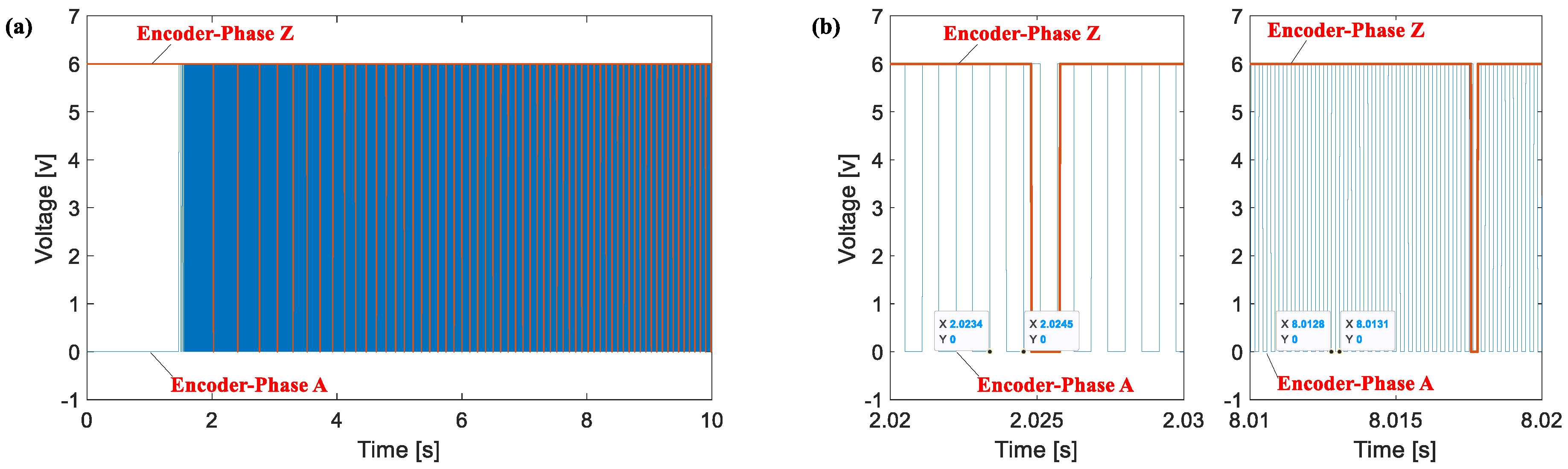
The principle of estimating rotational speed based on decoupling the gravity acceleration component from the tangential in situ accelerometer measurements is indeed feasible. By employing techniques such as filtering or signal processing algorithms, the gravity component can be separated from the tangential acceleration component, enabling the calculation of rotational speed.

(2)

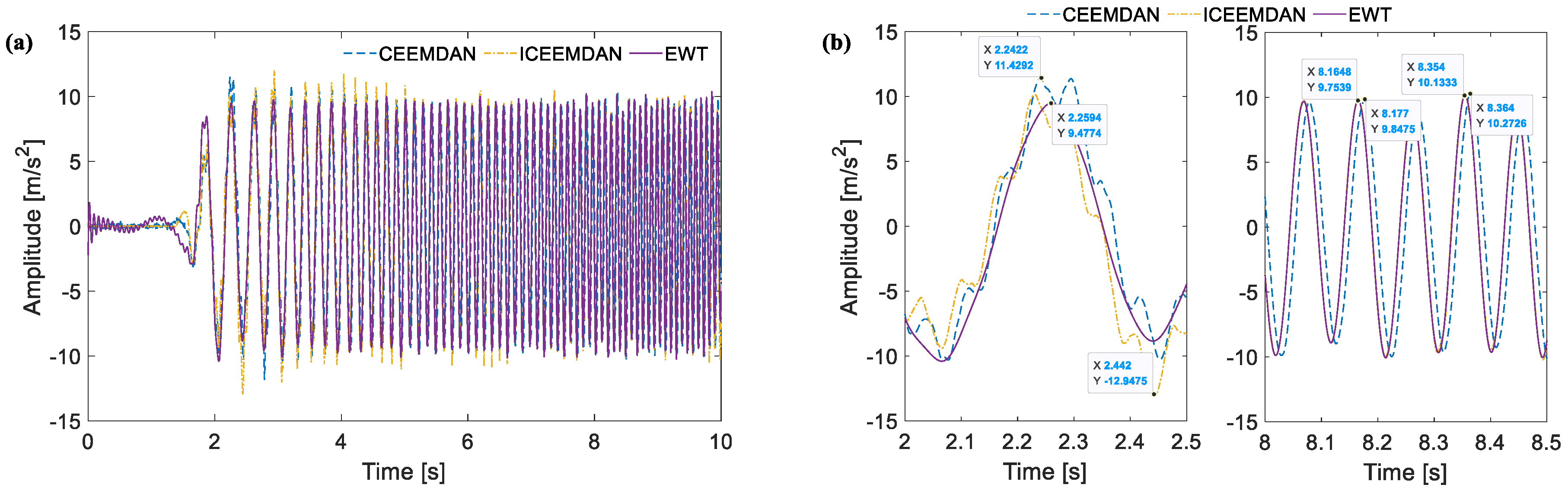
The utilization of the CEEMDAN, ICEEMDAN and EWT methods for decomposition and reconstruction reveals minimal differences among the three approaches. As a result, these minor variations are likely to have a negligible impact on the estimation errors of the rotational speed. This suggests that the choice of decomposition technique, within the range of these three methods, may not significantly affect the overall accuracy of rotational speed estimation.

(3)

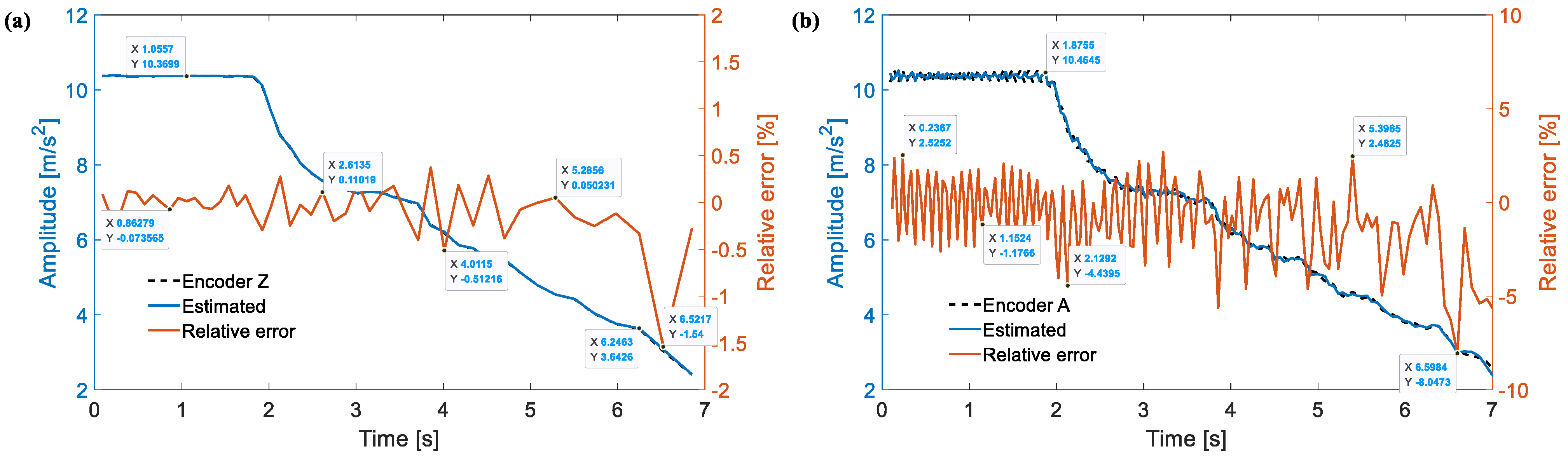
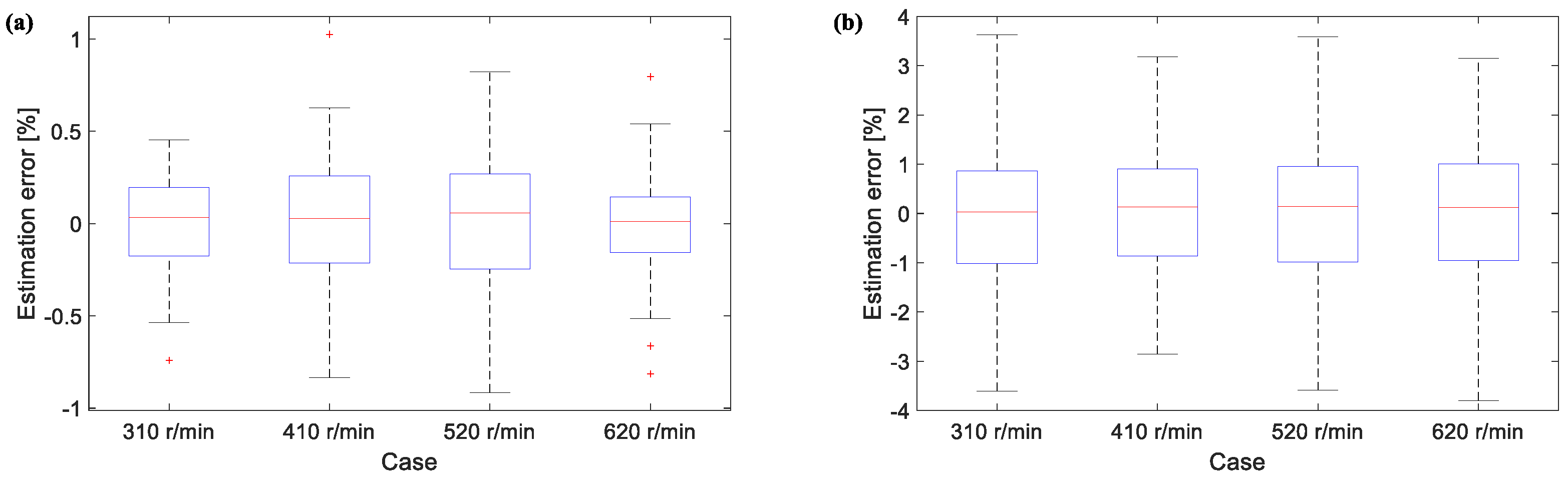
The proposed method demonstrates satisfactory estimation performance for both average and instantaneous rotational speeds. Specifically, the majority of the relative estimation errors for the average rotational speeds are confined to within ±0.5%, indicating a high level of accuracy. Similarly, for the instantaneous rotational speeds, most of the relative estimation errors are within ±5%, demonstrating a reasonable degree of precision compared to encoder-based measurement methods.

(4)

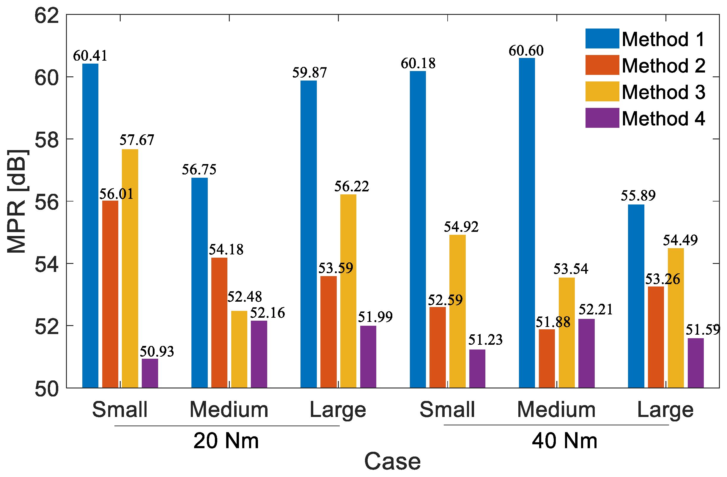
The proposed method exhibits superior performance in rotational speed estimation and order tracking within gearboxes, achieving an average gain of 5.36 dB over Method 2, 4.06 dB over Method 3 and a substantial 7.27 dB over Method 4.

Above all, the average and instantaneous rotational speeds can be well estimated based on the proposed GAD method, which offers good insights for enhancing fault detection and diagnostic capabilities in non-stationary applications.

References

1. Hong, L.; Qu, Y.Z.; Dhupia, J.S.; Sheng, S.; Tan, Y.; Zhou, Z. A novel vibration-based fault diagnostic algorithm for gearboxes under speed fluctuations without rotational speed measurement. Mech. Syst. Signal Process. 2017, 94, 14–32. [Google Scholar] [CrossRef]
2. Chen, Z.G.; Zhou, Z.W.; Zhai, W.M.; Wang, K. Improved analytical calculation model of spur gear mesh excitations with tooth profile deviations. Mech. Mach. Theory 2020, 149, 103838. [Google Scholar] [CrossRef]
3. Liu, J.; Wang, L.F.; Shi, Z.F. Dynamic modelling of the defect extension and appearance in a cylindrical roller bearing. Mech. Syst. Signal Process. 2022, 173, 109040. [Google Scholar] [CrossRef]
4. Liu, Y.Y.; Wen, H.; Ding, Z.Y.; Xu, L.; Chen, H.; Smulko, J. An Instantaneous Engine Speed Estimation Method Using Multiple Matching Synchrosqueezing Transform. J. Sens. 2021, 2021, 6650432. [Google Scholar] [CrossRef]
5. Singh, G.; Kumar, T.C.; Naikan, V.N. Speed estimation of rotating machinery using generated harmonics. Comput. Electr. Eng. 2018, 72, 420–430. [Google Scholar] [CrossRef]
6. Zeng, Q.; Feng, G.J.; Shao, Y.M.; Devitt, J.; Gu, F.; Ball, A. An accurate instantaneous angular speed estimation method based on a dual detector setup. Mech. Syst. Signal Process. 2020, 140, 106674. [Google Scholar] [CrossRef]
7. Zhao, M.; Jia, X.; Lin, J.; Lei, Y.; Lee, J. Instantaneous speed jitter detection via encoder signal and its application for the diagnosis of planetary gearbox. Mech. Syst. Signal Process. 2018, 98, 16–31. [Google Scholar] [CrossRef]
8. Shao, Y.M.; Su, D.Z.; Al-Habaibeh, A.; Yu, W. A new fault diagnosis algorithm for helical gears rotating at low speed using an optical encoder. Measurement 2016, 93, 449–459. [Google Scholar] [CrossRef]
9. Chin, Z.Y.; Smith, W.A.; Borghesani, P.; Randall, R.B.; Peng, Z. Absolute transmission error: A simple new tool for assessing gear wear. Mech. Syst. Signal Process. 2021, 146, 107070. [Google Scholar] [CrossRef]
10. Zhang, X.; Xu, G.H.; Chen, X.B.; Chen, R.; Xie, J.; Tian, P.; Zhang, S.; Wu, Q. Bearing fault diagnosis method based on angular domain resampling, relative position matrix and transfer learning. Meas. Sci. Technol. 2024, 35, 076118. [Google Scholar] [CrossRef]
11. Lu, S.L.; Yan, R.Q.; Liu, Y.B.; Wang, Q. Tacholess Speed Estimation in Order Tracking: A Review with Application to Rotating Machine Fault Diagnosis. IEEE Trans. Instrum. Meas. 2019, 68, 2315–2332. [Google Scholar] [CrossRef]
12. Lei, Y.G.; Li, N.P.; Guo, L.; Li, N.; Yan, T.; Lin, J. Machinery health prognostics: A systematic review from data acquisition to RUL prediction. Mech. Syst. Signal Process. 2018, 104, 799–834. [Google Scholar] [CrossRef]
13. Garcia-Calva, T.; Morinigo-Sotelo, D.; Mwata-Velu, T.; Garcia-Perez, A.; Uribe, K. Rotor speed estimation for half-broken bar detection in induction motors using Kalman filtering. Meas. Sci. Technol. 2024, 35, 076115. [Google Scholar] [CrossRef]
14. Wang, X.X.; Guo, J.; Lu, S.L.; Shen, C.; He, Q. A computer-vision-based rotating speed estimation method for motor bearing fault diagnosis. Meas. Sci. Technol. 2017, 28, 065012. [Google Scholar] [CrossRef]
15. Hu, Z.H.; Wang, J.X.; Wang, G.X.; Wen, S.; Li, Z. Extraction of time-frequency ridge line based on automatic peak search and curve fitting. Eng. Res. Express 2024, 6, 025502. [Google Scholar] [CrossRef]
16. Combet, F.; Zimroz, R. A new method for the estimation of the instantaneous speed relative fluctuation in a vibration signal based on the short time scale transform. Mech. Syst. Signal Process. 2009, 23, 1382–1397. [Google Scholar] [CrossRef]
17. Li, C.; Sanchez, V.; Zurita, G.; Lozada, M.C.; Cabrera, D. Rolling element bearing defect detection using the generalized synchrosqueezing transform guided by time-frequency ridge enhancement. ISA Trans. 2016, 60, 274–284. [Google Scholar] [CrossRef] [PubMed]
18. Urbanek, J.; Barszcz, T.; Antoni, J. A two-step procedure for estimation of instantaneous rotational speed with large fluctuations. Mech. Syst. Signal Process. 2013, 38, 96–102. [Google Scholar] [CrossRef]
19. Wang, Y.; Xu, G.H.; Zhang, Q.; Liu, D.; Jiang, K. Rotating speed isolation and its application to rolling element bearing fault diagnosis under large speed variation conditions. J. Sound Vib. 2015, 348, 381–396. [Google Scholar] [CrossRef]
20. Rodopoulos, K.; Yiakopoulos, C.; Antoniadis, I. A parametric approach for the estimation of the instantaneous speed of rotating machinery. Mech. Syst. Signal Process. 2014, 44, 31–46. [Google Scholar] [CrossRef]
21. Barrios, M.L.R.; Montero, F.E.H.; Mancilla, J.C.G.; Marín, E.P. Tacho-less automatic rotational speed estimation (TARSE) for a mechanical system with gear pair under non-stationary conditions. Measurement 2019, 145, 480–494. [Google Scholar] [CrossRef]
22. Mousavi, M.; Mostafavi, A.; Moradi, M.; Chaibakhsh, A.; Kordestani, M.; Derakhshanfar, M.; Saif, M. Robust Fault Isolation of Gas Turbines via Nonlinear Intelligent Observer and Takagi-Sugeno Fuzzy Inference System. IEEE Sens. J. 2023, 23, 25075–25085. [Google Scholar] [CrossRef]
23. Torres, M.E.; Colominas, M.A.; Schlotthauer, G.; Flandrin, P. A complete ensemble empirical mode decomposition with adaptive noise. In Proceedings of the 2011 IEEE International Conference on Acoustics, Speech and Signal Processing (ICASSP), Prague, Czech Republic, 22–27 May 2011; pp. 4144–4147. [Google Scholar]
24. Wang, L.M.; Shao, Y.M.; Cao, Z. Optimal demodulation subband selection for sun gear crack fault diagnosis in planetary gearbox. Measurement 2018, 125, 554–563. [Google Scholar] [CrossRef]
25. Rakshit, H.; Ullah, M.A. A Comparative Study on Window Functions for Designing Efficient FIR Filter. In Proceedings of the 2014 9th International Forum on Strategic Technology (IFOST), Cox’s Bazar, Bangladesh, 21–23 October 2014; pp. 91–96. [Google Scholar]
26. Wang, L.M.; Shao, Y.M. Fault feature extraction of rotating machinery using a reweighted complete ensemble empirical mode decomposition with adaptive noise and demodulation analysis. Mech. Syst. Signal Process. 2020, 138, 106545. [Google Scholar] [CrossRef]
27. Elouaham, S.; Nassiri, B.; Dliou, A.; Zougagh, H.; El Kamoun, N.; El Khadiri, K.; Said, S. Combination time frequency and empirical wavelet transform methods for removal of composite noise in EMG signals. TELKOMNIKA Telecommun. Comput. Electron. Control 2023, 21, 1373–1381. [Google Scholar] [CrossRef]
28. Gao, H.F.; Xu, T.X.; Li, R.L.; Cai, C. Gearbox Fault Diagnosis Based on ICEEMDAN-MPE-AWT and SE-ResNeXt50 Transfer Learning Model. Appl. Sci. 2024, 14, 2565. [Google Scholar] [CrossRef]
29. Zhang, X.; Miao, Q.; Zhang, H.; Wang, L. A parameter-adaptive VMD method based on grasshopper optimization algorithm to analyze vibration signals from rotating machinery. Mech. Syst. Signal Process. 2018, 108, 58–72. [Google Scholar] [CrossRef]
30. Schmidt, S.; Heyns, P.S.; De Villiers, J.P. A tacholess order tracking methodology based on a probabilistic approach to incorporate angular acceleration information into the maxima tracking process. Mech. Syst. Signal Process. 2018, 100, 630–646. [Google Scholar] [CrossRef]
31. Dliou, A.; Latif, R.; Laaboubi, M.; Maoulainine, F.; Elouaham, S. Noised abnormal ECG signal analysis by combining EMD and Choi-Williams techniques. In Proceedings of the 2012 IEEE International Conference on Complex Systems (ICCS), Agadir, Morocco, 5–6 November 2012; pp. 1–5. [Google Scholar] [CrossRef]
Figure 1. A schematic plot of the estimation principle based on an in situ MEMS accelerometer.
Applsci 14 04742 g001
Figure 2. A flowchart of the rotational speed estimation method and its application in order tracking.
Applsci 14 04742 g002
Figure 3. A schematic plot of the unwrapped phase angle of the gravity acceleration component.
Applsci 14 04742 g003
Figure 4. The established experimental setup: (a) sketch diagram; (b) photograph.
Applsci 14 04742 g004
Figure 5. The (a) acquired local embedded acceleration signals under the Test 01 working condition and (b) the zoomed-in plot.
Applsci 14 04742 g005
Figure 6. The (a) filtered local embedded acceleration signals and (b) the zoomed-in plot.
Applsci 14 04742 g006
Figure 7. The decomposed IMFs of the filtered local embedded acceleration signals: (a) IMFs 1~9 and (b) IMFs 10–18 based on CEEMDAN; (c) IMFs 1~8 and (d) IMFs 9–15 based on ICEEMDAN; (e) IMFs 1~8 and (f) IMFs 9–15 based on EWT.
Applsci 14 04742 g007aApplsci 14 04742 g007b
Figure 8. The calculated correlation coefficients of the IMFs and local embedded acceleration signals under Test 01: (a) CEEMDAN; (b) ICEEMDAN; (c) EWT.
Applsci 14 04742 g008
Figure 9. The (a) reconstructed time-varying gravity component under Test 01 based on the three methods and (b) the zoomed-in plot.
Applsci 14 04742 g009
Figure 10. The acquired encoder signal under the Test 01 working condition: (a) encoder signal; (b) zoomed-in plot.
Applsci 14 04742 g010
Figure 11. The estimated average and instantaneous rotational speeds for the Test 01 working condition: (a) average speed per revolution and (b) instantaneous speed.
Applsci 14 04742 g011
Figure 12. The (a) reconstructed gravity acceleration component under Test 02 and (b) the zoomed-in plot.
Applsci 14 04742 g012
Figure 13. The estimated average and instantaneous rotational speeds for the Test 02 working condition: (a) average speed per revolution and (b) instantaneous speed.
Applsci 14 04742 g013
Figure 14. The estimation errors based on the proposed method: (a) the estimated average speed and (b) the estimated instantaneous speed.
Applsci 14 04742 g014
Figure 15. (a) A schematic illustration of the test system and (b) photograph of the test system.
Applsci 14 04742 g015
Figure 16. A photograph of the wireless in situ acceleration test system.
Applsci 14 04742 g016
Figure 17. (a) A schematic diagram of the seeded spalling fault (b) photograph of the seeded spalling fault.
Applsci 14 04742 g017
Figure 18. Time domain waveforms of the in situ accelerometer under sped-up working conditions: (a) raw signal and (b) zoomed-in plot.
Applsci 14 04742 g018
Figure 19. The spectrum of the in situ accelerometer under sped-up working conditions: (a) raw signal and (b) zoomed-in plot.
Applsci 14 04742 g019
Figure 20. Acquired signals of the bearing housing accelerometer under sped-up working conditions: (a) time domain and (b) frequency spectrum.
Applsci 14 04742 g020
Figure 21. The (a) reconstructed time-varying gravity acceleration signal and (b) estimated rotational angle based on Method 1, (c) the estimated rotational speed and (d) angle based on Method 2, and (e) the estimated rotational speed and (f) angle based on Method 3, (g) the estimated rotational speed and (h) angle based on Method 4.
Applsci 14 04742 g021aApplsci 14 04742 g021b
Figure 22. A comparison between the original time domain signal and the resampled angle domain signal based on (a) Method 1, (b) Method 2, (c) Method 3 and (d) Method 4.
Applsci 14 04742 g022
Figure 23. The (a) order spectrum and (b) its envelope spectrum based on Method 1, (c) the order spectrum and (d) its envelope spectrum based on Method 2, (e) the order spectrum and (f) its envelope spectrum based on Method 3, and (g) the order spectrum and (h) its envelope spectrum based on Method 4.
Applsci 14 04742 g023aApplsci 14 04742 g023b
Figure 24. MPR values of the three methods in different working conditions.
Applsci 14 04742 g024