Abstract
Light field (LF) cameras can capture a scene’s information from all different directions and provide comprehensive image information. However, the resulting data processing commonly encounters problems of low contrast and low image quality. In this article, we put forward a content-adaptive light field contrast enhancement scheme using a focal stack (FS) and hierarchical structure. The proposed FS set contained 300 light field images, which were captured using a Lytro-Illum camera. In addition, we integrated the classical Stanford Lytro Light Field Archive and JPEG Pleno Database. Specifically, according to the global brightness, the acquired LF images were classified into four different categories. First, we transformed the original LF FS into a depth map (DMAP) and all-in-focus (AIF) image. The image category was preliminarily determined depending on the brightness information. Then, the adaptive parameters were acquired by the corresponding multilayer perceptron (MLP) network training, which intrinsically enhanced the contrast and adjusted the light field image. Finally, our method automatically produced an enhanced FS based on the DMAP and AIF image. The experimental comparison results demonstrate that the adaptive values predicted by our MLP had high precision and approached the ground truth. Moreover, compared to existing contrast enhancement methods, our method provides a global contrast enhancement, which improves, without over-enhancing, local areas. The complexity of image processing is reduced, and real-time, adaptive LF enhancement is realized.
1. Introduction
A light field (LF) captures all light data from different directions for each point of a scene [1]. The captured, four-dimensional data contain color and geometric structure information, such as direction and distance information. The unique advantages of LF make it useful in numerous applications, such as post-capture refocusing [2,3], 3D reconstruction [4], saliency detection [5], and motion deblurring [6]. The research on LF [7] focus stack (FS), depth map (DMAP), and all-in-focus (AIF) images has helped to reduce the high cost caused by huge data volumes. Keita Takahashi et al. [8] developed an LF display based on an FS; it can be simultaneously viewed from multiple directions without sacrificing resolution in any viewing direction. Google developed an immersive LF video [9], which can record, process, compress, and render view-dependent immersive LF videos at a sufficiently low bandwidth for internet streaming. The hologram company Looking Glass developed an immersive 3D hologram display using LF technology with life-like lighting and textures [10]. In general, current research shows that the light field is a promising medium for augmented and virtual reality.
With the rapid development of light field technology, LF cameras (Rattrix and Lytro, etc.) have attracted extensive attention because they can conveniently capture LF images in a single shot. Current cameras refocus by 2–6 captured views, which results in a low depth range (generally k = 2) and low precision of refocusing the foreground and background. However, LF cameras [11] refocus using LF sub-aperture images (SAIs), which have a wide depth range (generally k = 20–40) and high precision of pixel-level refocusing. Nevertheless, an LF image acquired using an LF camera has low image quality in terms of luminance contrast. Consequently, LF digital image enhancement has become the main research topic for obtaining information from image structures and to better interpret images.
In recent years, image contrast has been a popular research topic [12,13]. Contrast enhancement [14,15] is an important preprocessing procedure for a range of applications, such as remote sensing [16], medical imaging [17], and underwater imaging [18]. Among the numerous enhancement algorithms, histogram equalization (HE) is diffusely used [19,20]. However, HE is usually used to enhance the global contrast without selecting the data to process [21], which may lead to adverse effects, such as color bleeding, unnaturalness, a halo effect, or over-enhancement [22]. In addition, the existing contrast enhancement schemes are all for 2D images, and there is no research on LF image processing. Therefore, a real-time and intelligent algorithm with which to heighten the contrast is required, which will improve the LF image quality and boost information representation.
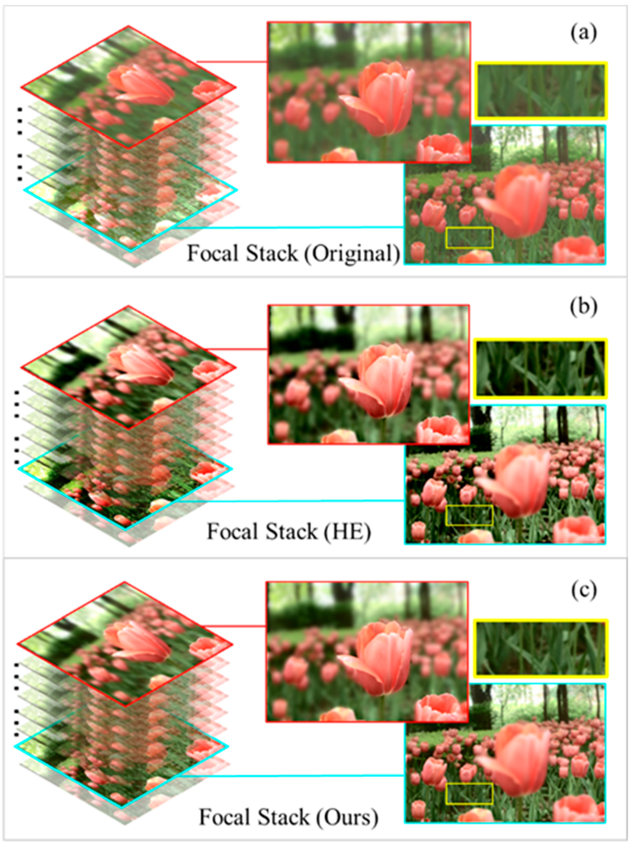
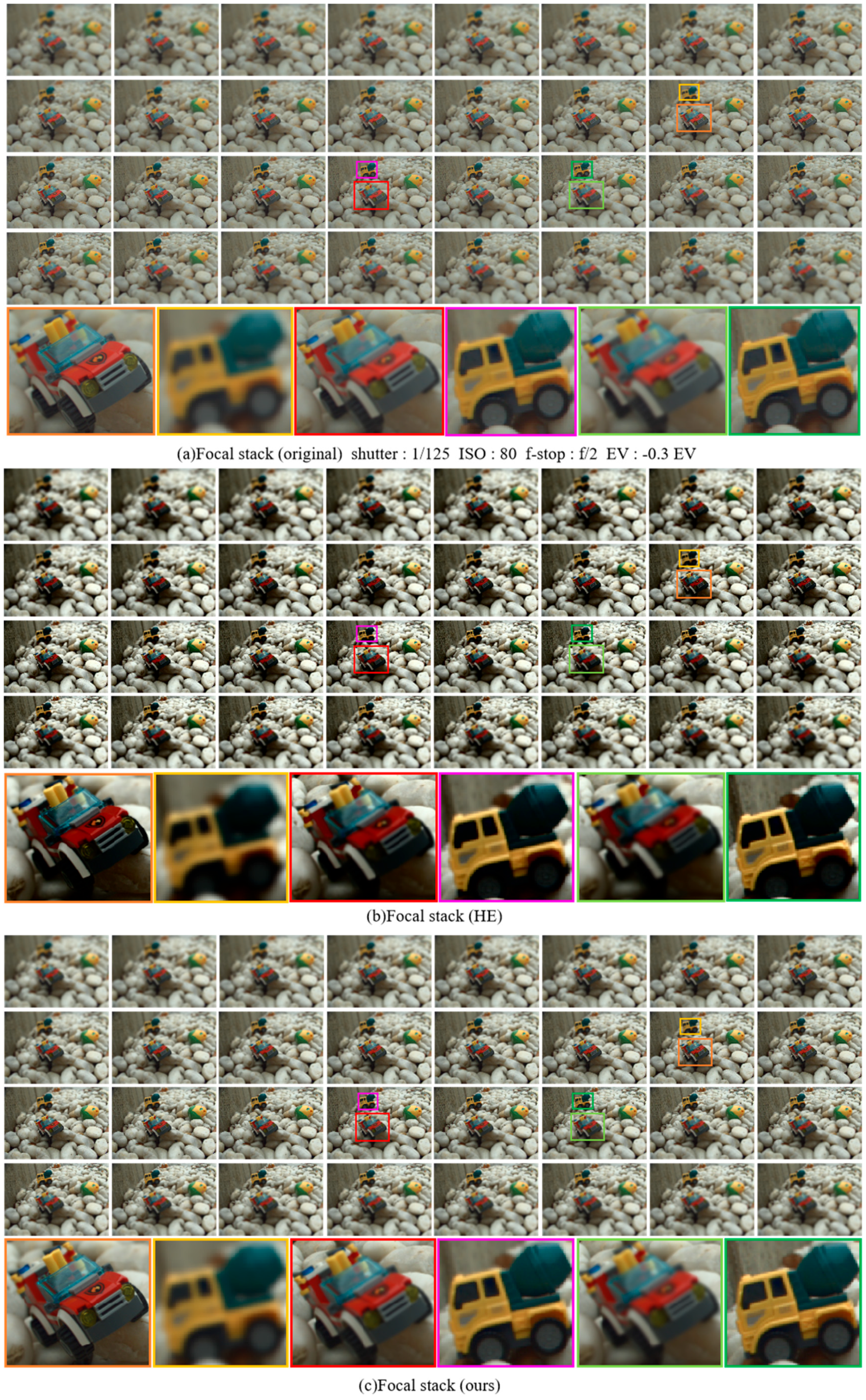
We present a content-adaptive LF contrast enhancement method to boost the information expression, and the adaptive parameters are predicted by a hierarchical network in this article. First, the database images are divided into four categories according to the image feature information. Then, we take the multilayer perceptron (MLP) based on a previous classification to obtain the adaptive parameters and enhance the image contrast intelligently. This method realizes batch dispose and automatically operates on multiple images, which greatly improves the image processing speed. As illustrated in Figure 1, focal stack comparison results show the effectiveness of our scheme. The global contrast of the enhanced FS is significantly improved. The enhanced focus stack obtained by our method has better image quality for dark areas. The texture of the greenery is depressed in (b) but clear in (c). The over-enhanced regions in (b) are recovered by our adjustments. Most notably, the application of our proposed contrast algorithm to LF image enhancement is an original and novel contribution, to the best of our knowledge. A preliminary version of this paper was published at an international conference [23]. This paper provides an in-depth discussion, a more complete description, and supplementary experimental results. The main contributions of the work are as follows:
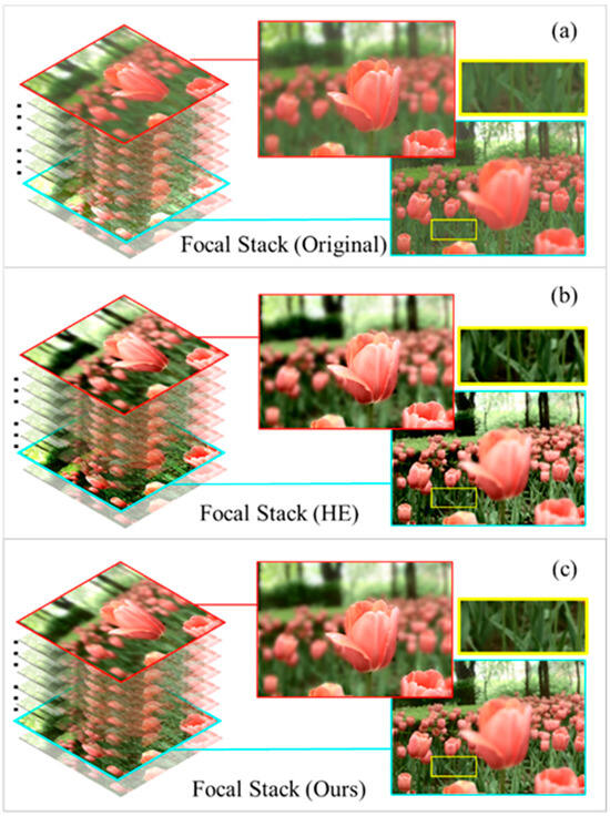
Figure 1.
Comparison of the effect of the contrast enhancement method. (a) Original LF focal stack; (b) the focal stack obtained after HE; (c) our resulting focal stack.
- (1)
- This paper proposes a novel, adaptive LF contrast enhancement method by using an MLP to train the dataset, which automatically adapts to mapping the curve parameters of the different views, adjusts the image ulteriorly, and enhances the contrast.
- (2)
- According to the global brightness, we build a new LF dataset that acquires and classifies LF images into four different categories based on an MLP network. Our own database, which is the classical Stanford Lytro Light Field Archive and JPEG Pleno Database embedding, is also applied in this work.
- (3)
- Contrast enhancement is applied to the LF FS. The comparison experimental results for the original and synthetic images show that our method is a state-of-the-art method.
2. Related Work
2.1. LF Imaging
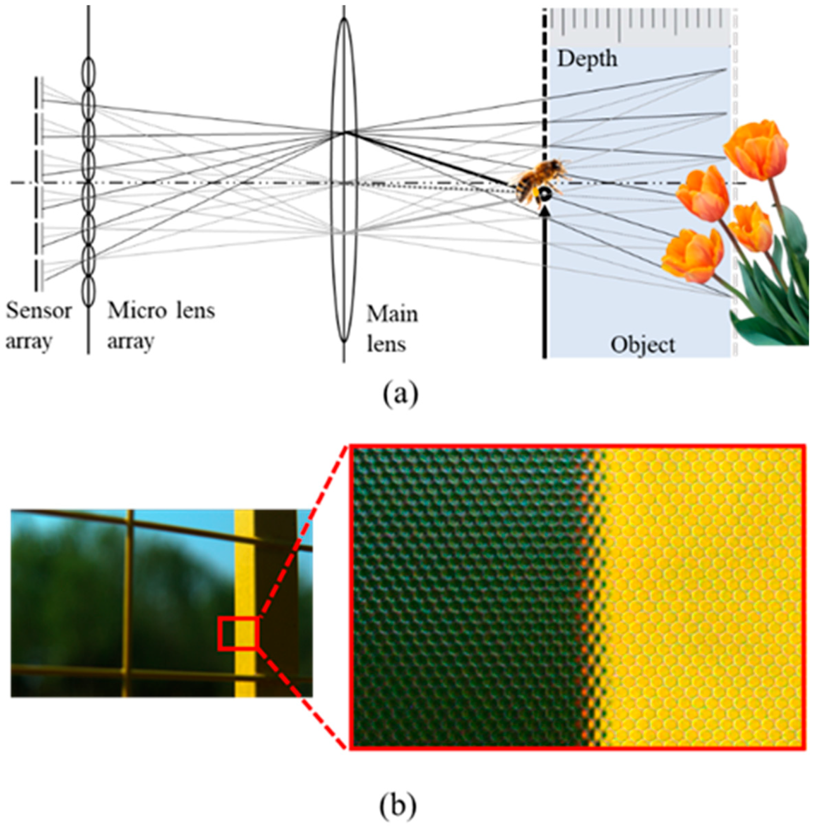
As illustrated in Figure 2a, LF imaging records light [24] by adding a microlens array and subsequently performs digital zooming using a post-processing algorithm (Fourier slice theorem, LF imaging algorithm). According to the principle of LF imaging, refocused or sub-aperture images are realized based on the recorded light to obtain LF images for research. Chi Zhang et al. [25] proposed an efficient auto-refocusing (ARF) solution for LF cameras, where only three refocus renders are required to find the best refocus frame. Yingqian Wang et al. [2] presented an LF refocusing solution to improve image quality. This method can selectively refocus the image, super-resolve the focused region, and aesthetically render the bokeh. Shachar Ben Dayan et al. [26] put forward a neural network digital refocusing algorithm based on sparse angular information; its structure is relatively small and can be quickly reconstructed with low memory consumption.
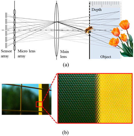
Figure 2.
(a) Light field imaging principle; (b)original image decoded by LF camera.
In our experimental study, several classes of scenes were taken using a Lytro-Illum camera (using a tripod as an auxiliary tool) in order to establish a new dataset. The camera parameter set, scenes, and features of the LF image (sunshine, cloudy, and indoor) are illustrated in Table 1 below. The camera saved the gained data in files with the suffix LFP (about 55 MB each), which contained several types of data (such as RAW images, thumbnails in BMP format, system settings, etc.). The RAW image is 10-bit packages, with a total resolution of 7728 × 5368 in GRBG format. The Light Field Toolbox for Matlab v0.5 [27] was utilized to process the RAW files. The package generated our required 5D files, as well as other additional files (such as color-corrected images, etc.), by decoding and correcting the LF data, using the camera’s calibration information (a series of white image files taken from the Lytro-Illum’s external memory card).

Table 1.
Lytro-Illum camera parameter set, scenes, and features of LF images.
The output of the decoding was the reconstructed LF corresponding to the square grid of the microlens (5D file above). The square grid consisted of 625 × 434 microlenses, and each microlens captured light information from 15 × 15 different directions. The data were saved in the matrix LF (i, j, k, l, c) of size (15, 15, 434, 625, 4) [28]. Figure 2b shows the reconstructed light field; the original data decoded by the LF camera comprises the individual circular areas. The reason for this is that each microlens images the circular main lens, and the final image produced by the LF camera is actually the sum of the pixels that correspond to each microlens. In other words, one microlens is one pixel of the final LF image. However, the size limitation of the microlens results in the low resolution and low quality of the final imaging.
2.2. LF Image Enhancement
2.2.1. Super-Resolution
Due to the characteristics of the LF camera, the original LF image obtained by decoding has low resolution [29]. Youngjin Yoon et al. [30] presented a novel algorithm for LF super-resolution (SR) using a deep convolutional neural architecture. The spatial and angular SR network is concatenated to jointly improve the resolution. Gaosheng Liu et al. [31] introduced a new idea for light field angular SR and presented an efficient LF angular SR architecture, which is called EASR. This method achieves efficient angular super-resolution by giving an excellent trade-off between reconstruction performance and inference time.
2.2.2. Color and Low-Light Enhancement
LF is easily affected by low illumination and noise. Light field enhancement in low illumination is more untoward than a single image task, due to the need to address a series of problems, such as color distortion, noise, and multiple views. Shansi Zhang et al. [32] proposed a learning-based algorithm for LF image decomposition enhancement. Low-light LF images with different light intensities are synthesized by simulating the imaging process [33]. This method can effectively recover the geometric structure, spatial details, brightness, and color of the images under multifarious illumination levels. Xianglang Wang et al. [34] developed a novel light field algorithm for low-light enhancement and denoising using a multi-stream progressive restoration method. This model outperforms the state-of-the-art method on both real-world low-light LF datasets and synthetic-noise light field datasets.
2.2.3. Contrast Enhancement
The decoded LF image also has low quality. Researchers hope to heighten the image information expression by enhancing the image contrast. The research on the contrast of LF images is limited, so we expanded the contrast enhancement algorithm to ordinary images. Among the numerous contrast enhancement algorithms, HE is the basic strategy for most enhancement techniques in image processing. On account of its effectiveness and simplicity, histogram equalization is one of the most widely used techniques to achieve contrast enhancement [35]. HE modifies the histogram to improve the limited dynamic range of the image. The original image histogram can be transformed into a uniform distribution (equilibrium) form, and the dynamic range of the gray value difference between pixels can be increased to heighten the contrast of the image by using HE. Many attempts [12,36,37,38] have been based on this method to improve the visual quality. However, HE enhances the details excessively, which augments background interference and reduces the detailed data. In this paper, to the best of our knowledge, we apply adaptive image enhancement for the first time and resolve the inherent problems of the HE method for LF images.
2.3. Adaptive Image Enhancement
Image processing is a repetitive, labor-intensive, and time-consuming process. We introduce a novel, adaptive LF contrast enhancement method using a MLP network. Complex and repetitive work can be reduced by introducing machine learning models. Yue Wu et al. [39] presented a nearest neighbor search and match method (NNA), which has low computational complexity and strong robustness. Alireza Sepas-Moghaddam et al. [40] presented the first deep convolution neural network (CNN) solution for LF-based face recognition. This method has superior performance for face recognition and simplifies complex algorithms. In this paper, the mapping curve is automatically adjusted by predicting the adaptive parameters of the model to improve the image contrast. Our adaptive enhancement algorithm is different from the contrast enhancement methods in [13,37] in the following ways. (1) A different network structure: a machine learning link is introduced to realize the batch processing and real-time operation of multiple images, which greatly improves the image processing speed. (2) A different process: different enhancement intensities are adopted for different images according to the image characteristics, instead of adopting a unified processing mode.
3. Proposed Method
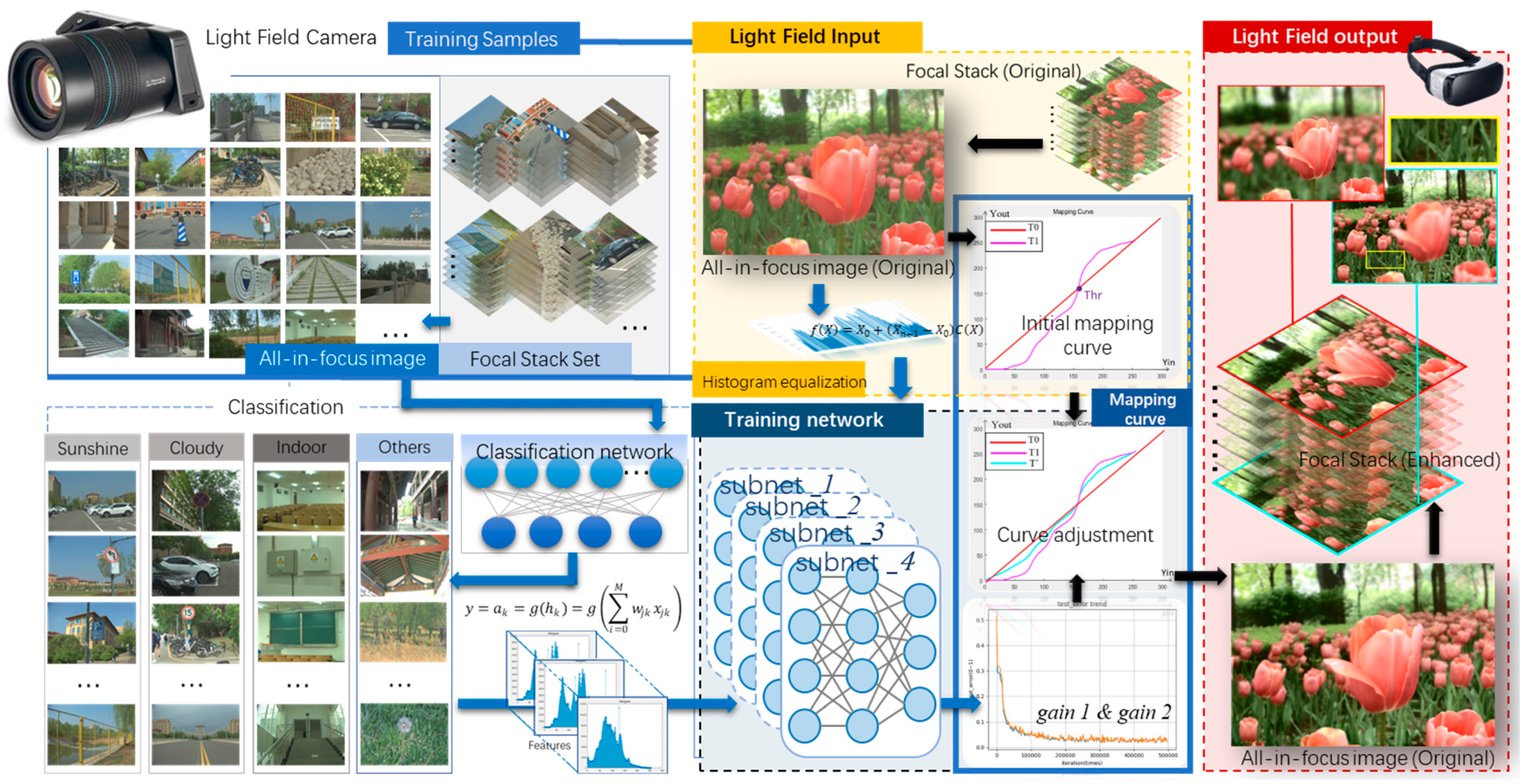
Figure 3 illustrates the framework of the prosed enhancement process of LF FS. The original FS set is captured by a light field Lytro-Illum camera, and the AIF image is further generated. We obtain the adaptive parameters using a hierarchical network. The first layer of the network classifies the FS dataset into four different categories based on the MLP network. The second layer predicts the adaptive parameters, and the features that are fed to the network are extracted from the brightness information of the original LF AIF image. Next, the image enhancement is shown. The HE is adopted to acquire the initial mapping curve. Then, the adaptive parameters are used to adjust the curve to acquire the enhanced AIF image. Finally, the FS is restored via the AIF image. First, in this section, we will introduce the image contrast enhancement algorithm, and then propose the machine learning model to acquire the adaptive parameters.
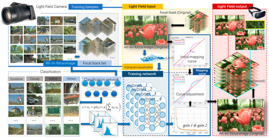
Figure 3.
Framework of the proposed content-adaptive light field FS contrast enhancement.
3.1. FS Transforms into AIF
For the LF camera decoding after the preliminary processing to acquire the raw FS, the FS includes 32 images with different depths. If each image is enhanced, the steps are identical and reduplicative. Therefore, we generate the full-focus image from the raw FS, enhance the contrast of the AIF image, and subsequently convert it into the FS using the DMAP and enhanced full-focus image, which can effectively extract the features of LF images and cover the most information with less work.
A focus stack is a series of images focused on different planes. Therefore, the original image of the light field is refocused 32 times, and this series of refocused images is called the focus stack. The gradient of each pixel in the focus stack is calculated, and then the gradient image of each image is filtered by the mean value. Then, the sum of the squares of the gradient values of the three channels is calculated and the mean value is taken, and the square root is taken, which is the gradient value of the image. The maximum gradient of the pixel at the same position of the focus stack means that the pixel is the clearest at that depth; that is to say, the object at that depth surface is the clearest. The index value of the depth is recorded, from which the depth map can be synthesized.
In most cases, DMAPs can be directly downloaded from many datasets and with the raw LF data, e.g., [41], although some LF images do not have DMAPs. To ensure the diversity of the application range of the proposed scheme, the DMAPs in this paper are extracted from the LF dataset instead of being directly downloaded from the Lytro camera. We adopt the method of Zhao, C. et al. [42,43], and use the FS to simultaneously render the AIF image and DMAP. The AIF image refers to the set of all the best in-focus pixels in the FS, i.e., the best in-focus pixel at every position is gathered. Suppose there are K refocused images in the FS, where the k-th refocused image is named , α is defined as the relative depth, and its distance from the aperture plane is F’ = αF:
We use the difference focus measure to obtain the focus map , which is the discrepancy between two focus maps, one from the FS and the other from the guided-filtered FS , designed to cancel out the discrepancy.
where , . Here, maintains the boundaries while smoothing the others through a guided filter , and it is denoted as . indicates a focus measure of choice; the ring difference filter is chosen due to its robustness, coming from incorporating local and non-local characteristics into the filtering window in this paper.
For one pixel at position (x, y), the best in-focus pixel value is elected from , , …, by referring to the focus map In the selection of K refocused images of the image, at position (x,y), we focus on the biggest pixels at the best focus pixel and image index, and use , which is defined as
The AIF image can be formed by collecting the pixels at the best in-focus at all positions, as described by
where represents the best focus pixel at position (x,y). The DMAP is the set of pixel indices at the maximum focus of all images in the FS, that is
3.2. Statistical Feature Extraction
In this part, contrast enhancement is performed on the above AIF image. In the contrast enhancement method based on HE [13,44], the cumulative distribution function is used to change the histogram distribution into an approximate uniform distribution to enhance the contrast. However, the gray level of the transformed image is reduced, which makes some details disappear. If some images have high peaks in their histograms, the contrast will be unnaturally over-enhanced. This paper proposes an improved method considering these shortcomings. We adjust the local details by changing the mapping curve obtained by HE, which not only retains the superior performance of the enhanced part, but also reduces the amplitude of the over-enhanced part.
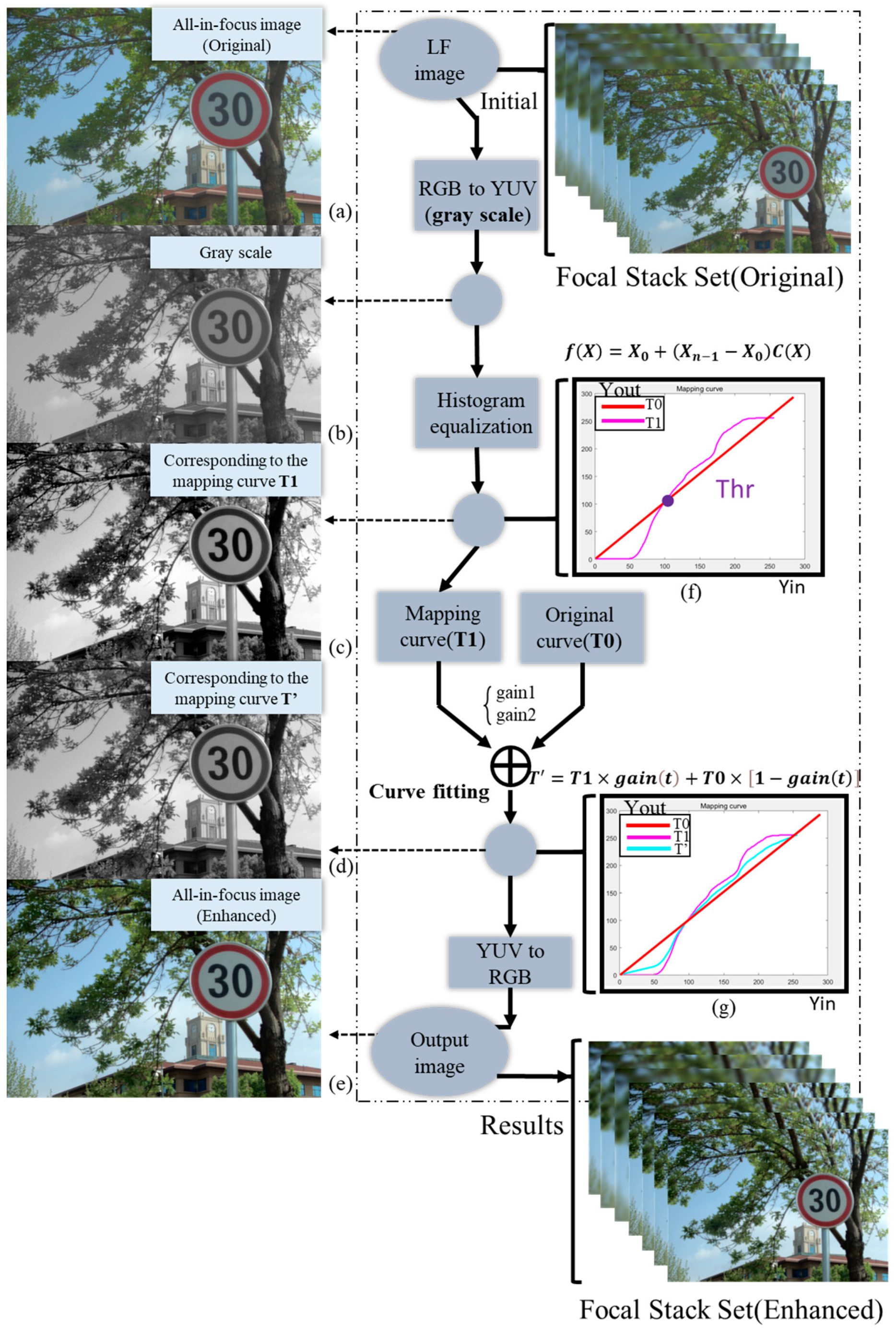
As shown in Figure 4, the AIF image is obtained from the original FS by using the method in Section 3.1. We transform the original RGB image into a YUV format image, and then form the grayscale image (b). For image (b), considering the input, its range of grayscale is , which has n pixels in total. The probability density function of level is
where n is the sum of pixels in the image, and is the frequency of occurrence of level ; k = 0, 1, …, N − 1. The histogram is the relationship between and . On the basis of (6), the cumulative density function is
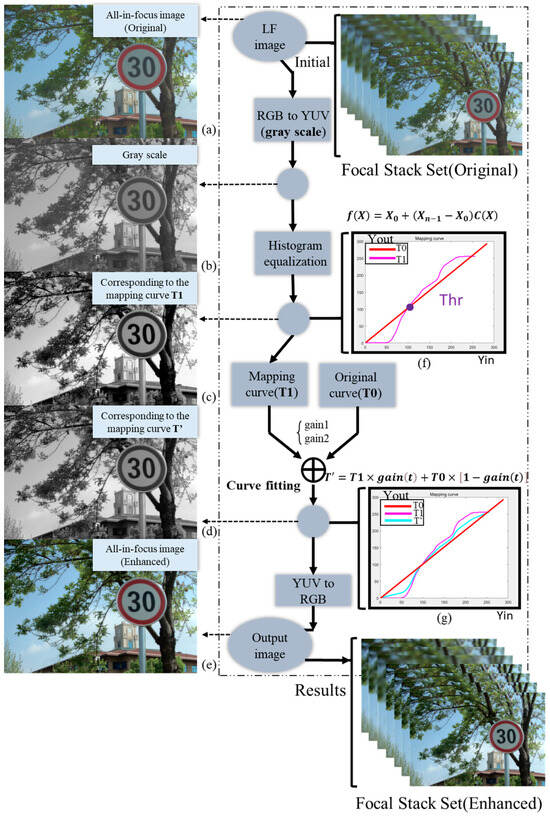
Figure 4.
Flowchart of the contrast enhancement method. (a) Original AIF image; (b) Grey-scale map; (c) Grey-scale map after HE; (d) Grey-scale map after our method; (e) Enhanced AIF image. (f,g) represent formulas and algorithms used in the processing process (f) = Equation (8), (g) = Equation (9).
HE uses the cumulative density function to map the image pixel values onto the entire dynamic range , as
Image (c) and the mapping curve, accordingly, are obtained using the above steps, and we subsequently adjust the mapping curve. As shown in Figure 4, is the original curve, and represents the mapped curve after histogram equalization.
Yin = Yout; the output is the original AIF image at this time. Two parameters are adopted to adjust the mapping curve. Gain1 is used to adjust the brighter part, while gain2 is applied to adjust the darker part of the image. By comparing the curves and and selecting suitable values, the adjusted curve T’ is attained
where t is 0 or 1, and gain (t) is 0–1 to adjust the dark and bright parts, respectively. The optimized enhanced image (d) can be acquired by using this scheme, and subsequently recover the RGB image (e), which is the resulting light field image. The enhanced AIF image can be obtained by using this method. Then, the method of Zhao et al. [42] is used to generate the FS through AIF and DMAP.
3.3. Hierarchical Network
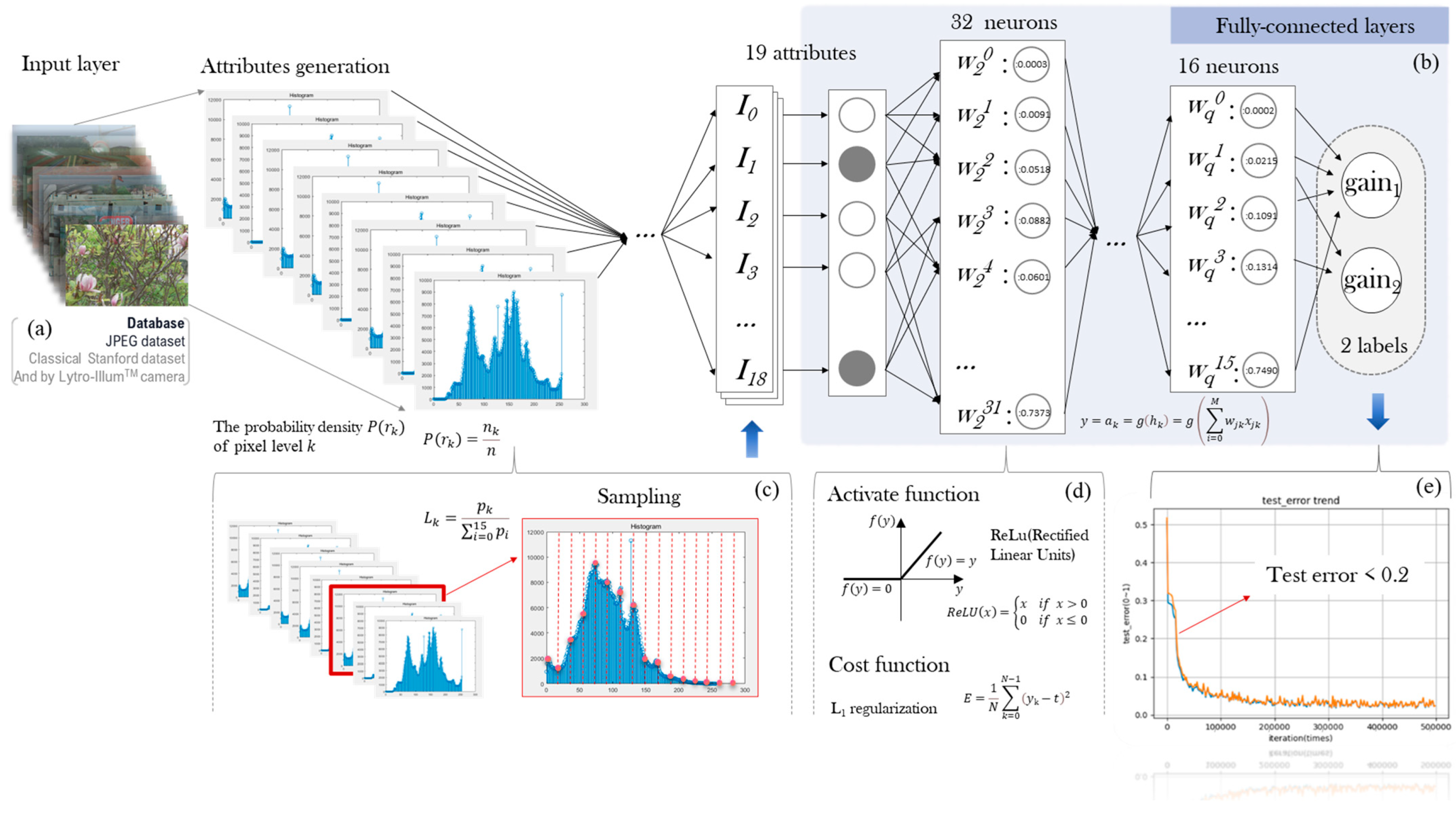
There are top and bottom networks in our hierarchical architecture. Firstly, the top layer of the hierarchical network function is trained as a classifier of the LF dataset into four categories based on the global brightness (as shown in Figure 3): sunny day, cloudy day, indoor, and other. Secondly, according to the separate training for the four image types, the next layer function is further trained for the adaptive parameter values of the selected gain systems. As Figure 5 shows, a key processing step for obtaining gain1 and gain2 in our multilayer perceptron network is formed. By inputting the hybrid database of the LF image, we extract the characteristic information and conduct a further sampling, making use of 19 attributes of the fully connected layers. Each training pair consists of the feature data as the input and the corresponding target values for gain1 and gain2 as the output. The distribution of image brightness is correlated with the adaptive parameters directly utilized for adjusting the mapping curve and subsequently enhancing the image contrast, thereby effectively mitigating the excessive contrast between light and dark regions in the LF image.

Figure 5.
Architecture of multilayer perceptron network and feature extraction. (a) Database; (b) Fully-connected layers; (c) Feature extraction; (d) Activate function and cost function; (e) Test error.
3.3.1. Database Collection
In the training process, as depicted in Figure 5a, the classical Stanford dataset and the JPEG dataset [40,45], which are commonly used LF image datasets, along with the images from our Lytro-Illum camera, are selected as the training database (DB). The “crop and resize operation” [44] augmentation method is applied to enlarge the DB.
3.3.2. Ground Truth Setting and Training Pair
This paper modifies the mapping curve of the AIF image by setting the gain value to enhance the contrast of the LF image, utilizing gain1 and gain2 as the ground truth. The target of the architecture is to predict parameter values for gain1 and gain2 from the input original AIF image. During training, the input features encompass brightness information extracted from the original AIF images; contain 16 histogram values (); and the maximum, minimum, as well as the average brightness (), as illustrated in Figure 5c.
where denotes the k-th bin histogram value.
3.3.3. The Input and Output Layers
The input is the above 19 groups of feature data representing image brightness, and the adaptive values are the output. The output value y is given by
where g( ) is the activation function; this paper chooses the widely used rectified Linear Activation Unit (ReLU).
As shown in Figure 5d, ReLU is the most commonly used activation function for training convolutional layers and deep learning models. It offers the advantages of simplicity of computation and ease of optimization, particularly when the behavior of neural networks is linear or near-linear. Therefore, it is well suited for performing supervised tasks on large-scale labeled datasets. Here, x denotes the input, w is the weight, signifies the total of the output weight of k neurons in the output layer, and represents the current number of neurons and the weight of neurons in the next layer. As illustrated in Figure 5b, the value of q is 3 in our study. The loss function E adopts the sum-of-squares error function
We define the following metrics:
- True positive (TP): A positive example of being correctly predicted. That is, the true value of the data is a positive example, and the predicted value is also a positive example.
- True negative (TN): Counterexamples that were correctly predicted. That is, the true value of the data is a counter example, and the predicted value is also a counter example.
- False Positive (FP): Positive example of misprediction. That is, the real value of the data is a negative example, but it is wrongly predicted as a positive example.
- False negative (FN): A counterexample of being incorrectly predicted. That is, the true value of the data is a positive example, but it is incorrectly predicted to be a negative example.
According to the above metrics, the accuracy is 0.91. It can be seen that the prediction result of the machine learning network model is more reliable. Due to the balance of hardware overhead and effects, the current accuracy is sufficient to meet current needs, and we will consider further improving accuracy in the future.
Finally, utilizing 19 sets of data, using the characteristic data of the image as the input and gain1 and gain2 as the output, the LF images are trained via the aforementioned MLP network to establish the relationship between the input and output. According to Figure 5e, the test error of the parameters acquired by the multilayer perceptron-trained network is less than 0.2, which shows that reliable values can be obtained using this method. The experiment is performed on our LF dataset, integrated with the classical LF dataset, which comprises 300 images of four scenes, including diverse conditions, such as sunny, cloudy, and indoor. Each image in the dataset undergoes augmentation as described above. Subsequently, 90% of the results are allocated for training, and the remaining 10% are used for testing. A substantial amount of training results are processed to derive the exact adaptive parameters.
4. Experimental Results and Discussion
We trained the network on 300 images (70 from the JPEG Pleno Database [41], 86 from the classical Stanford Lytro Light Field Archive [45], and 144 taken by ourselves); the training results were applied to 26 images (6 images from the JPEG Pleno Database [41], 5 images from the classical Stanford Lytro Light Field Archive [45], and 15 images taken by ourselves). From the resulting obtained FS, the global contrast of the light field image was enhanced appropriately without the over-enhancement of local regions. The image information expression was more comprehensive, and the hidden details were recovered by histogram stretching. Next, we will evaluate the quality of the results through a subjective and objective assessment.
4.1. Subjective Assessment
While it would be desirable to have an objective assessment method to compare contrast enhancement techniques, unfortunately there is no accepted objective criterion in the literature that can provide meaningful results for each image [13]. On this basis, we have tried to find more suitable objective evaluation criteria to evaluate image quality. In terms of the subjective evaluation experiment, we designed a questionnaire and invited 50 people to respond to the questionnaire to evaluate the light field images obtained by the proposed method and the HE, CLAHE, and Imadjust methods. The results show that 85% of the people thought that the image quality obtained by our method was better, and 10% of the people thought that the image results obtained by the CLAHE method were better. A total of 5% considered the image quality obtained by the Imadjust method to be better. The results show that our method is more consistent with human viewing logic and has a better visual effect.
Figure 6 shows the original LF images and their various corresponding contrast-enhanced images. We compared our method with HE [19], the contrast enhancement algorithm (Imadjust) proposed by P.R. Rothe et al. [46], and the classical contrast-limited adaptive histogram equalization (CLAHE) enhancement algorithm [47,48]. In general, the HE of an image can best utilize the dynamic range of pixel values for maximum contrast. However, the generated images generally have low visual quality. This finding can also be seen in Figure 6c. The amplification of noise reduces the image quality, and undesired artifacts become more prominent, which results in an unnatural appearance. As shown in Figure 6b,d, steps were taken to ameliorate the situation, such as using the proposed CLAHE and Imadjust methods. The Imadjust method significantly improved the image over-enhancement, but the details were also erased. For example, the details of the bricks under cloudy conditions completely disappeared. We found that in many of the tested images, both CLAHE and our method showed similar quality and were close to the real sensation. However, our scheme yielded better overall contrast, whereas the CLAHE method had a light image color and a poor contrast effect. In addition, there were some problems, such as unnatural color transition, seen in the flowers and leaves in Figure 6b under cloudy conditions. Figure 7 illustrates the FS for contrast enhancement. Since our method was implemented based on HE, we compared it with the HE method. The contrast between the two was effectively enhanced (especially HE), and hidden details (such as stone texture) were revealed.
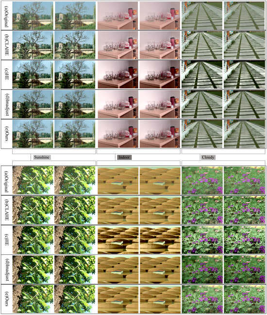
Figure 6.
Comparison of focal stack results. (a) Original image; (b) CLAHE method; (c) HE method; (d) Imadjust method; (e) our method.
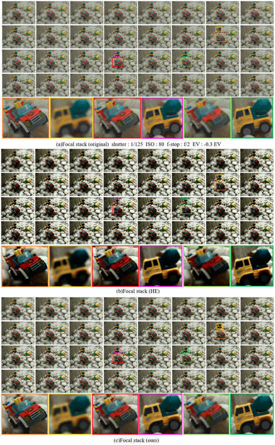
Figure 7.
Focal stack comparison. (a) Original focal stack; (b) HE focal stack; (c) our focal stack.
However, the HE algorithm only considers the image contrast, which causes excessive enhancement and drowns out some details of the image. On the contrary, the contrast of the image after our processing was effectively enhanced without changing the naturalness, such as the texture of the car tire and the details of the wall, which completely disappeared after HE. However, our method enhanced the contrast while enhancing the information expression and deepening the details of the original image.
4.2. Objective Assessment
An effective enhancement algorithm should improve the perceived quality without affecting the naturalness of the image or adding any artifacts [49]. Nonetheless, relying on a subjective judgment of image quality is not sufficiently accurate, since the judgment of each individual varies greatly. Table 2 shows the data results, and we made the following objective assessments of the images.
Table 2.
Image quality evaluation of the proposed algorithms compared with CLAHE, HE, and Imadjust.
Ideally, the contrast enhancement method should not change the hole brightness. The Absolute Mean Brightness Error (AMBE) calculates the brightness change, which is defined as the difference between the mean intensity of the original image and that of the enhanced image .
where E(.) is the mean intensity of the underlying image. A lower AMBE indicates better corresponding brightness preservation. The results show that this evaluation criterion is consistent with the subjective assessment. The HE method has poor brightness preservation, while our method and CLAHE have better expression. The average brightness is effectively maintained, and the enhanced image can better restore the overall brightness characteristics of the original image, and has better adaptability to the human eye.
The most obvious metric by which to access a contrast enhancement architecture is contrast improvement. S. S Agaian et al. [50] proposed a method to evaluate the contrast of complex images called the Measure of Enhancement by Entropy (EMEE), and defined it for the enhanced image as
where the symbols max and min correspond to the maximum and minimum intensity values, M and N are the width and height, C is a constant to avoid division by zero, and α is an exponent to control for the enhancement effect [50]. Using this evaluation criterion, HE achieves the best presentation, although it may produce unreal appearances and may not produce visually pleasing images. This finding is understandable, because HE does not consider whether the image is natural and real, and only aims to improve the contrast. The results show that our method improves the image contrast and does not produce an unnatural appearance. This result can be seen in Figure 7; although the contrast of the LF image is greatly improved, the detailed information in the LF image is lost due to the excessive contrast enhancement of the LF image after the HE method, and the texture of the cars, stones, and other objects disappears.
H. D. Cheng et al. [51] devised an objective criterion with which to detect over-enhancement, which is called the Structure Measure Operator (SMO) and is defined as
where is the product of three values: the entropy, edge value, and standard deviation around a pixel in a d × d window. The SMO is insensitive to changes in contrast, but sensitive to changes in structure. Ideally, the SMO is zero if the enhancement does not change the structure. The results show that over-enhancement occurs with the HE method, and the other methods show a high performance, which is consistent with our subjective analysis.
To evaluate the preservation of image naturalness, C. Bai et al. [52] presented the Lightness Order Measure (LOM) from a local inversion of the lightness order.
where is the difference between the pixel values of the original and its local mean-filtered version and, similarly, is for the enhanced component. Here, sign(.) is the signum function. The lower the LOM value, the better the image naturalness preservation. The results indicate that CLAHE and our method realize the optimal naturalness preservation.
4.3. Cost Effectiveness Analysis
In this paper, an effective adaptive values acquisition is developed by multilayer perceptron network training, which simplifies and lowers the time required for image processing. The most crucial point is that HE, CLAHE, and Imadjust are not targeted and use a single processing mode, whereas our method can perform advisable contrast enhancement based on the specific features of each light field image. The results indicate that the proposed method can improve the overall contrast of the image effectively. From a cost–benefit viewpoint, our adaptive enhancement algorithm utilizes an MLP network to predict parameter implementation in real time. The architecture is devised with a light structure, which reduces the cost waste, and it can precisely obtain the parameters. The light field image batch processing is realized, which greatly shortens the image processing time.
5. Conclusions
Our adaptive LF contrast enhancement method uses an efficient hierarchical training structure based on MLP, and the hierarchical structure improves the parameter acquisition accuracy to enhance the contrast of LF images. The experimental results show that it is superior to existing methods for facilitating image processing and appropriately enhancing the global contrast without losing details. Meanwhile, the MLP network achieves adaptive LF enhancement, which is user friendly and real time. Our architecture can be used to implement real-time enhanced portal devices with limited hardware resources.
Light field images have wide application prospects, such as Google’s development of LF immersive video calls [53], Samsung’s development of a slim-panel holographic video display [54], and Light Field Lab’s SolidLight that offers a true holographic video display [55]. In the future, we would like to enhance the scalability of our approach. For example, the FS formed by our method currently has a low resolution (624 × 432), and we want to enhance the image contrast while increasing the resolution. Because low-light LF images lack information expression and produce more noise due to the dark shooting light, we hope to enhance the information expression by improving the contrast of the low-light field image and denoising. In the future, we will implement light field composite enhancement suitable for various scenes.
Author Contributions
Conceptualization, X.G. and Z.Y.; methodology, X.G.; software, X.G.; investigation, X.G. and J.G.; resources, Z.Y.; data curation, X.G.; writing—original draft preparation, X.G. and J.G.; writing—review and editing, Z.Y. and Y.C.; supervision, Z.Y. and Y.C.; project administration, Z.Y. All authors have read and agreed to the published version of the manuscript.
Funding
This research was funded by the Key Research and Development Program of Shanxi Province, grant number 202102150401011, and the National Natural Science Foundation of China, grant number 52275568.
Institutional Review Board Statement
Not applicable.
Informed Consent Statement
Not applicable.
Data Availability Statement
The raw data supporting the conclusions of this article will be made available by the authors on request.
Acknowledgments
The author would also like to thank Runfang Hao for his proofreading comments during the review process of the paper and for his help with the related calculations in the machine learning part.
Conflicts of Interest
The authors declare no conflicts of interest.
References
- Zhao, C.; Jeon, B. Refocusing metric of light field image using region-adaptive multi-scale focus measure. IEEE Access 2022, 10, 101385–101398. [Google Scholar] [CrossRef]
- Wang, Y.; Yang, J.; Guo, Y.; Xiao, C.; An, W. Selective light field refocusing for camera arrays using bokeh rendering and superresolution. IEEE Signal Process Lett. 2019, 26, 204–208. [Google Scholar] [CrossRef]
- Jayaweera, S.; Edussooriya, C.; Wijenayake, C.; Agathoklis, P.; Bruton, L. Multi-volumetric refocusing of light fields. IEEE Signal Process Lett. 2021, 28, 31–35. [Google Scholar] [CrossRef]
- Kim, C.; Zimmer, H.; Pritch, Y.; Sorkine-Hornung, A.; Gross, M.H. Scene reconstruction from high spatio-angular resolution light fields. ACM Trans. Graph. 2013, 32, 1–12. [Google Scholar] [CrossRef]
- Li, N.; Ye, J.; Ji, Y.; Ling, H.; Yu, J. Saliency detection on light field. In Proceedings of the IEEE Conference on Computer Vision and Pattern Recognition, Columbus, OH, USA, 24–27 June 2014; pp. 1605–1616. [Google Scholar]
- Srinivasan, P.P.; Ng, R.; Ramamoorthi, R. Light field blind motion deblurring. In Proceedings of the IEEE Conference on Computer Vision and Pattern Recognition (CVPR), Honolulu, HI, USA, 21–26 July 2017. [Google Scholar]
- Schambach, M.; Heizmann, M. A multispectral light field dataset and framework for light field deep learning. IEEE Access 2020, 8, 193492–193502. [Google Scholar] [CrossRef]
- Takahashi, K.; Kobayashi, Y.; Fujii, T. From focal stack to tensor light-field display. IEEE Trans. Image Process 2018, 27, 4571–4584. [Google Scholar] [CrossRef] [PubMed]
- Michael, B.; John, F.; Ryan, O.; Daniel, E.; Peter, H.; Matthew, D.; Jason, D.; Jay, B.; Matt, W.; Paul, D. Immersive light field video with a layered mesh representation. ACM Trans. Graph. 2020, 39, 86:1–86:15. [Google Scholar]
- Spatial without the Headset. Available online: https://lookingglassfactory.com/ (accessed on 23 May 2024).
- Todor, G.; Yu, Z.; Lumsdaine, A.; Goma, S. Lytro camera technology: Theory, algorithms, performance analysis. Multimed. Content Mob. Devices 2013, 8667, 458–467. [Google Scholar]
- Celik, T.; Tjahjadi, T. Automatic image equalization and contrast enhancement using Gaussian mixture modeling. IEEE Trans. Image Process 2012, 21, 145–156. [Google Scholar] [CrossRef] [PubMed]
- Arici, T.; Dikbas, S.; Altunbasak, Y. A histogram modification framework and its application for image contrast enhancement. IEEE Trans. Image Process 2009, 18, 1921–1935. [Google Scholar] [CrossRef] [PubMed]
- Fay, L.; Cobos, E.; Yang, B.; Gatidis, S.; Küstner, T. Avoiding shortcut-learning by mutual information minimization in deep learning-based image processing. IEEE Access 2023, 11, 64070–64086. [Google Scholar] [CrossRef]
- Jiang, C.; Han, J.-J. A multiobject detection scheme based on deep learning for infrared images. IEEE Access 2022, 10, 78939–78952. [Google Scholar] [CrossRef]
- Liu, J.; Zhou, C.; Chen, P.; Kang, C. An efficient contrast enhancement method for remote sensing images. IEEE Geosci. Remote Sens. Lett. 2017, 14, 1715–1719. [Google Scholar] [CrossRef]
- Naseem, R.; Cheikh, F.A.; Beghdadi, A.; Elle, O.J.; Lindseth, F. Cross modality guided liver image enhancement of ct using mri. In Proceedings of the European Workshop on Visual Information Processing (EUVIP), Roma, Italy, 28–31 October 2019. [Google Scholar]
- Singh, B.; Mishra, R.S.; Gour, P. Analysis of contrast enhancement techniques for underwater image. Int. J. Comput. Technol. Electron. Eng. 2011, 1, 190–194. [Google Scholar]
- Shanmugavadivu, P.; Balasubramanian, K. Thresholded and optimized histogram equalization for contrast enhancement of images. Comput. Electr. Eng. 2014, 40, 757–768. [Google Scholar] [CrossRef]
- Dyke, R.M.; Hormann, K. Histogram equalization using a selective filter. Vis. Comput. 2023, 39, 6221–6235. [Google Scholar] [CrossRef] [PubMed]
- Wang, W.; Yang, Y. A histogram equalization model for color image contrast enhancement. Signal Image Video Process. 2024, 18, 1725–1732. [Google Scholar] [CrossRef]
- Cheng, H.D.; Shi, X.J. A simple and effective histogram equalization approach to image enhancement. Digit. Signal Process. 2004, 14, 158–170. [Google Scholar] [CrossRef]
- Guo, X.; Zhao, C.; Cheng, Y.; Xu, M.; Yuan, Z. Adaptive light field contrast enhancement using efficient feature extraction. In Proceedings of the IEEE International Symposium on Broadband Multimedia Systems and Broadcasting (BMSB), Beijing, China, 14–16 June 2023. [Google Scholar]
- Hahne, C.; Aggoun, A. PlenoptiCam v1.0: A light-field imaging framework. IEEE Trans. Image Process 2021, 30, 6757–6771. [Google Scholar] [CrossRef] [PubMed]
- Zhang, C.; Hou, G.; Zhang, Z.; Sun, Z.; Tan, T. Efficient auto-refocusing for light field camera. Pattern Recognit. 2018, 81, 176–189. [Google Scholar] [CrossRef]
- Dayan, S.; Mendlovic, D.; Giryes, R. Deep sparse light field refocusing. arXiv 2020, arXiv:2009.02582. [Google Scholar]
- Dansereau, D.G.; Pizarro, O.; Williams, S.B. Decoding, calibration and rectification for lenselet-based plenoptic cameras. In Proceedings of the IEEE Conference on Computer Vision and Pattern Recognition (CVPR), Portland, OR, USA, 23–28 June 2013. [Google Scholar]
- Vieira, A.; Duarte, H.; Perra, C.; Tavora, L.; Assuncao, P. Data formats for high efficiency coding of Lytro-Illum light fields. In Proceedings of the International Conference on Image Processing Theory, Tools and Applications (IPTA), Orleans, France, 10–13 November 2015. [Google Scholar]
- Jiang, Y.; Gong, X.; Liu, D.; Cheng, Y.; Fang, C.; Shen, X.; Yang, J.; Zhou, P.; Wang, Z. EnlightenGAN: Deep Light Enhancement Without Paired Supervision. IEEE Trans. Image Process. 2021, 30, 2340–2349. [Google Scholar] [CrossRef] [PubMed]
- Yoon, Y.; Jeon, H.-G.; Yoo, D.; Lee, J.-Y.; Kweon, I.S. Learning a deep convolutional network for light-field image super-resolution. In Proceedings of the IEEE International Conference on Computer Vision Workshop (ICCVW), Santiago, Chile, 7–13 December 2015. [Google Scholar]
- Liu, G.; Yue, H.; Wu, J.; Yang, J. Efficient light field angular super-resolution with sub-aperture feature learning and macro-pixel upsampling. IEEE Trans. Multimed. 2022, 25, 6588–6600. [Google Scholar] [CrossRef]
- Zhang, S.; Lam, E. Learning to restore light fields under low-light imaging. Neurocomputing 2021, 456, 76–87. [Google Scholar] [CrossRef]
- Lv, F.; Li, Y.; Lu, F. Attention guided low-light Image enhancement with a large scale low-light simulation dataset. Int. J. Comput. Vis. 2021, 129, 2175–2193. [Google Scholar] [CrossRef]
- Wang, X.; Lin, Y.; Zhang, S. Multi-stream progressive restoration for low-light light field enhancement and denoising. IEEE Trans. Comput. Imaging 2023, 9, 70–82. [Google Scholar] [CrossRef]
- Kim, Y.-T. Contrast enhancement using brightness preserving bi-histogram equalization. IEEE Trans. Consum. Electron. 1997, 43, 1–8. [Google Scholar]
- Wang, Y.; Chen, Q.; Zhang, B. Image enhancement based on equal area dualistic sub-image histogram equalization method. IEEE Trans. Consum. Electron. 1999, 45, 68–75. [Google Scholar] [CrossRef]
- Stark, J.A. Adaptive image contrast enhancement using generalizations of histogram equalization. IEEE Trans. Image Process 2000, 9, 889–896. [Google Scholar] [CrossRef] [PubMed]
- Lee, C.; Lee, C.; Kim, C. Contrast enhancement based on layered difference representation of 2d histograms. IEEE Trans. Image Process 2013, 22, 5372–5384. [Google Scholar] [CrossRef] [PubMed]
- Wu, Y. Research on feature point extraction and matching machine learning method based on light field imaging. Neural Comput. Appl. 2019, 31, 8157–8169. [Google Scholar] [CrossRef]
- Sepas-Moghaddam, A.; Correia, P.L.; Nasrollahi, K.; Moeslund, T.B.; Pereira, F. Light field based face representation. In Proceedings of the IEEE 28th International Workshop on Machine Learning for Signal Processing (MLSP), Aalborg, Denmark, 17–20 September 2018. [Google Scholar]
- Řeřábek, M.; Ebrahimi, T. New light field image dataset. In Proceedings of the International Workshop on Quality of Multimedia Experience (QoMEX), Lisbon, Portugal, 6–8 June 2016. [Google Scholar]
- Zhao, C.; Jeon, B. A practical light field representation and coding scheme with an emphasis on refocusing. IEIE Trans. Smart Process. Comput. 2022, 11, 305–315. [Google Scholar] [CrossRef]
- Zhao, C.; Jeon, B. Compact Representation of Light Field Data for Refocusing and Focal Stack Reconstruction Using Depth Adaptive Multi-CNN. IEEE Trans. 2024, 10, 170–180. [Google Scholar] [CrossRef]
- Abdullah-Al-Wadud, M.; Kabir, M.H.; Dewan, M.A.A.; Chae, O. A dynamic histogram equalization for image contrast enhancement. IEEE Trans. Consum. Electron. 2007, 53, 593–600. [Google Scholar] [CrossRef]
- The (New) Stanford Light Field Archive. Available online: http://lightfield.stanford.edu/ (accessed on 27 January 2024).
- Rothe, P.R.; Kshirsagar, R.V. A study on the method of image pre-processing for recognition of crop diseases. In Proceedings of the IJCA Proceedings on International Conference on Benchmarks in Engineering Science and Technology (ICBEST), Kumasi, Ghana, 25–27 October 2012. [Google Scholar]
- Sahu, S.; Singh, A.K.; Ghrera, S.P.; Elhoseny, M. An approach for de-noising and contrast enhancement of retinal fundus image using CLAHE. Opt. Laser Technol. 2019, 110, 87–98. [Google Scholar]
- Pizer, S.M.; Johnston, R.E.; Ericksen, J.P.; Yankaskas, B.C.; Muller, K.E. Contrast-limited adaptive histogram equalization: Speed and effectiveness. In Proceedings of the First Conference on Visualization in Biomedical Computing, Atlanta, GA, USA, 22–25 May 1990. [Google Scholar]
- Khan, Z.A.; Beghdadi, A.; Cheikh, F.A.; Kaaniche, M.; Qureshi, M.A. A multi-criteria contrast enhancement evaluation measure using wavelet decomposition. In Proceedings of the IEEE 22nd International Workshop on Multimedia Signal Processing (MMSP), Tampere, Finland, 21–24 September 2020. [Google Scholar]
- Agaian, S.S.; Silver, B.; Panetta, K.A. Transform coefficient histogram-based image enhancement algorithms using contrast entropy. IEEE Trans. Image Process. 2007, 16, 741–758. [Google Scholar] [CrossRef] [PubMed]
- Cheng, H.-D.; Zhang, Y. Detecting of contrast over-enhancement. In Proceedings of the IEEE International Conference on Image Processing, Orlando, FL, USA, 30 September–3 October 2012. [Google Scholar]
- Bai, C.; Reibman, A.R. Controllable image illumination enhancement with an over-enhancement measure. In Proceedings of the IEEE International Conference on Image Processing (ICIP), Athens, Greece, 7–10 October 2018. [Google Scholar]
- Google’s Impressive 3D Video Conference—Here’s How it Works. Available online: https://www.techradar.com/news/googles-impressive-3d-video-conference-heres-how-it-works (accessed on 14 January 2024).
- Samsung Develops a Slim-Panel Holographic Video Display. Available online: https://techxplore.com/news/2020-11-samsung-slim-panel-holographic-video.html (accessed on 28 January 2024).
- Light Field Lab’s Solid Light Offers a True Holographic Video Display. Available online: https://www.techhive.com/article/579894/light-field-labs-solidlight-offers-a-true-holographic-video-display.html (accessed on 26 January 2024).

Disclaimer/Publisher’s Note: The statements, opinions and data contained in all publications are solely those of the individual author(s) and contributor(s) and not of MDPI and/or the editor(s). MDPI and/or the editor(s) disclaim responsibility for any injury to people or property resulting from any ideas, methods, instructions or products referred to in the content. |
© 2024 by the authors. Licensee MDPI, Basel, Switzerland. This article is an open access article distributed under the terms and conditions of the Creative Commons Attribution (CC BY) license (https://creativecommons.org/licenses/by/4.0/).