Abstract
The vibrations of plate structures placed in a supersonic flow was considered. The undisturbed fluid flow was parallel to the plate. This type of problem is especially important in the aerospace industry, where it is named panel flutter. It has been noticed for a long time that panel flutter may be problematic at high speeds. In this article, two specific problems were treated: in the first one, the plate was in the form of an infinite strip and the flow was in the direction of its finite length. Rigid walls indefinitely extended from the sides of the plate. In the second problem, the plate was a finite rectangle and the flow was parallel to one of its sides. The rest of the plane of the rectangle was again rigid. The first problem was a limiting case of the second problem. The flow was modeled by piston theory, which assumes that the fluid pressure on the plate is proportional to its local slope. This approximation is widely used at high speeds (supersonic speeds in the range of M > 1), and reduces the interaction between the fluid flow and the vibrations of the plate to an additional term in the vibration equation. The resulting problem can be solved by assumed mode methods. In this study, the solution was also found by using the collocation method. The contribution of this study is the correlation between the flutter velocity and the other parameters of the plate. The main result is the flutter velocity of the free fluid flow under which the plate vibrations become unstable. Finally, simple expressions are proposed between the various non-dimensional parameters that allows for the quick estimation of the flutter velocity. These simple expressions were deduced by least squares fits to the computed flutter velocities.
1. Introduction
Fluid–elastic structure interactions are ubiquitous in many engineering disciplines. There are historically famous examples that demonstrate that the interaction between fluid flow and the vibrations of the structure can cause catastrophic failure. It is observed that the character of vibrations typically depend on a characteristic flow velocity that, if it exceeds a certain value (the flutter velocity), will cause instability. The main thrust of fluid–elastic structure interaction research is the determination of the flutter velocity. This study’s innovation lies in the correlation between the flutter velocity and other model properties. The literature defines supersonic speeds as M > 1.2, and thus, the speed range pertains to Mach numbers greater than 1.2.
The type of problem considered in this study is especially important in aerospace structures and is usually given the name panel flutter. Panel flutter has been an active area of research, starting with the development of high-speed projectiles and rockets around the 1950s. A well-known publication that summarizes the theory and the general methods of solution is [1]. A more recent text is [2]. The AGARD (Advisory Group for Aerospace Research and Development—NATO) publication is an engineering manual dealing with the detection and alleviation of aeroelasticity problems, including experimental methods and various collected tables and graphs [3]. The literature on panel and plate flutter is immense; some of the recent work relevant to the problems considered in this study is summarized here: Uzal et al. dealt with incompressible and irrotational flow in a cylindrical channel to analytically find the flutter velocity [4]. Epureanu et al. investigated vibration-based damage with their chances in material and/or stiffness properties of structures. Kapkin et al. investigated the membrane vibrations located at the stagnation point of the flow and they give the flutter velocity for the system [5]. Vedeneev considered panel flutter at low supersonic speeds by using piston theory [6]. E. H. Dowell gave flutter velocity graphs for an infinite plate lying in the same direction as the fluid motion by using the potential theory for different Mach numbers [7]. Durak B. investigated plate vibrations by using potential flow theory in his PhD thesis [8]. Kapkin et al. tried to find a similar equation to predict the flutter velocity for a membrane with a stagnation flow [9]. Uzal et al. give an analytical solution for a plate placed in a rigid channel that fluid flows in [10]. Also, some of the researchers are also trying to avoid this flutter point by applying a force or moving one boundary to control the motion of the plate. Uzal and Korbahti controlled the resonance frequencies of a rectangular plate’s vibrations by applying a discrete force by measuring the displacement of the plate at a point [11]. Sezgin et al. give a boundary backstepping control method to stabilize the flow-induced vibrations for a membrane [12]. Tubaldi et al. investigated a periodically supported flexible plate under flowing fluid axial flow that is in a channel bounded by a rigid wall [13]. Lin et al. investigated how to control the oscillations of a two-dimensional ribbed plate with free boundary conditions by using a point-wise control method [14]. Li used the Rayleigh–Ritz method to determine the modal characteristics of a rectangular plate with elastic boundary supports [15]. The effects of the system parameters on the stability of the plate are discussed.
In this study, we considered the vibrations of infinite strip plates and rectangular finite plates under the effect of a high-speed flow parallel to the plate. The plate vibrations were modeled by the well-known linear (infinite strip) and two-dimensional (finite rectangle) plate vibration equations. The infinite strip was infinite in the direction perpendicular to the flow and the infinite sides were assumed to be simply supported. The finite rectangular plate was simply supported at all its sides. In both cases, the plates were made up of homogeneous, isotropic, linear material. The flow was taken to be in the high supersonic regime, and was modeled by employing piston theory, according to which, the local pressure was proportional to the local slope of the plate. This allowed for including the coupling between the plate vibrations and the fluid flow simply as an additional term in the plate vibration equation. The bare vibration equations were fourth order in space and second order in time; therefore, their solutions were in the form of undamped vibrations, neither growing nor decreasing in time. In contrast, the vibration equations including the piston theory terms contained first-order derivatives in time and space. This allowed for the solutions to decrease or blow-up in time. We were interested in the boundary between these two regimes, which gives the stability boundary, and the flutter velocity, which was the main quantity of interest.
This paper is organized as follows: In Section 2, we present general formulations for the fluid–structure systems under consideration. And a useful approximate theory of aerodynamics, the piston theory approach, is given in Section 3. In Section 4, the governing equations for the infinite strip case are given and non-dimensionalized in a suitable fashion, and the solution using the point collocation method is presented. In Section 5, the case of the finite rectangular plate is also similarly described. Both cases can also be solved analytically; these are presented in Section 6. Thus, analytical and approximate methods of solution (in the present case, the collocation method) could be compared. Section 7 presents the analytical and numerical results (the non-dimensional flutter velocity against a non-dimensional mass ratio) for both problems; also, the convergence of the collocation results to the analytical solution is demonstrated. Finally, inspired by the structure of the flutter curves, simple equations relating the non-dimensional flutter velocity to the mass ratio are developed for both the strip and rectangle cases. The rectangle case also includes another non-dimensional parameter: the ratio of the sides of the rectangle.
2. General Formulation
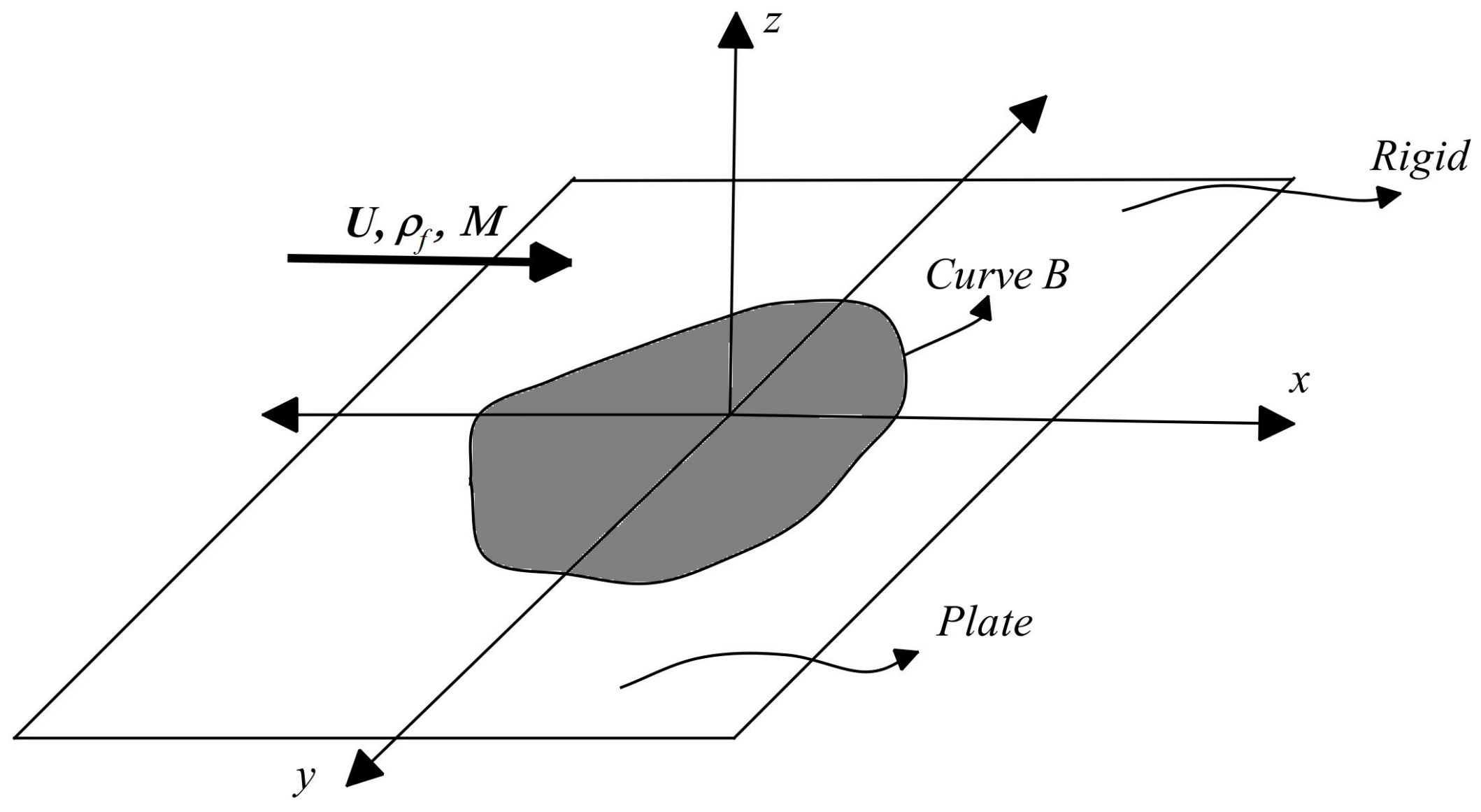
Many fluid–solid coupled vibration problems have the general form shown in Figure 1.

Figure 1.
General form for fluid–solid coupled vibration problems.
The fluid flows (in the undisturbed case) parallel to a rigid plane (which is taken as the xy-plane), with an elastic plate occupying the region bounded by a closed curve B. The flow direction is taken as the x-axis. The flow causes vibrations on the plate, which, in turn, slightly modifies (disturbs) the flow. Under certain conditions, more mechanical energy is transferred from the fluid to the plate, causing the magnitude of the vibrations of the plate to increase, usually exponentially. In the actual nonlinear case, the growing vibrations may be bounded by nonlinear interactions (or they may lead to structural failure), but this is still an unwanted situation from an engineering standpoint. Therefore, investigating the linearized fluid–elastic body coupling phenomena is of great engineering and scientific interest. The most general case may be formulated as follows: The flow is modeled by the compressible potential equation:
where is the velocity potential
The local speed of sound a is given by
This is because the predominant force that causes the plate to vibrate is the fluid pressure; viscous stresses would normally have little effect since they are mainly in the flow direction. Therefore, unless there are large-scale flow separations, which is not the case here, the viscous effects and other sources of vorticity can be ignored and the flow can be assumed to be potential. The differentiation of the pressure with respect to density is done at constant entropy (isentropic). In the potential equation, the speed of sound is to be eliminated by using the compressible Bernoulli equation:
The plate vibrations, in the case of an elastic, linear, and isotropic plate material, are governed by
where denotes the plate displacement, D is the plate bending rigidity, and is the density of the plate (). P is the fluid pressure on the plate surface.
We assumed that the plate boundaries are simply supported by the rigid extensions, which means that the plate displacement and the bending moment are zero at the boundaries. Finally, at the plate surface, the normal components of the plate and fluid velocities must be the same:
Here, is the unit vector in the z-direction, n is the vector normal to the plate surface (while it is vibrating), and V is the fluid velocity. Note that the conditions between the fluid and the solid (pressure expression and the velocity condition) makes the problem nonlinear, in addition to the velocity potential equation. To arrive at a tractable (i.e., linear) but still physical model, we assumed that the plate vibration amplitude was small enough so that the potential equation could be linearized around the uniform flow in the x-direction:
where is the sound velocity in free stream conditions. As a natural extension of this assumption, the pressure on the plate was assumed to be the pressure at :
and the velocity condition on the plate and fluid was also linearized:
The problem expressed by these equations can be attacked by first expressing the velocity potential in terms of the plate displacement by means of a two-dimensional Fourier transform in x and y, computing the pressure from Bernoulli’s equation, and then substituting its value at z = 0 into the plate vibration equation. Since the expression for the velocity potential involves double integrals, including the plate displacement, the final form of the plate vibration equation is a partial integro-differential eigenvalue problem.
3. Piston Theory Approximation
The integro-differential equation mentioned in the last section is more or less the most general formulation of the plate flutter problem. But it is quite a difficult mathematical problem. This type of plate vibration problem is usually termed as panel flutter in the aerospace industry, and it is well known that panel flutter is important at high supersonic speeds [16]. A useful approximate aerodynamic theory exists in this regime known as piston theory [17]. Developed in 1956, piston theory asserts that at high supersonic speeds, the local pressure is proportional to the slope of the boundary ((13) below). With the piston theory approximation, the potential flow equation is discarded and the vibrations are governed by a modified form of the plate vibration equation ((14) below). Note that the usual plate vibration equation contains only second-order derivatives; therefore, it can only exhibit steady time-harmonic vibrations. The modified equation above also has first-order derivatives, and it can, in principle, model attenuated or amplified vibrations; the latter case corresponds to panel flutter.
4. Infinite Strip Plate
Figure 2 shows a schematic of the first problem. The flow occupies the region and is in the x-direction with uniform velocity U. The region in the -plane with and is an elastic plate (infinite strip) of width b; the rest of the -plane is rigid. The vibrations of the plate cause small perturbations in the flow velocity. Some different equations can be found in the literature to define the vibrations of the plates [18,19,20,21,22,23,24]. The vibrations of the plate are governed by [18,19,20]
where is the displacement, is the thickness, is the density of the plate, and
is the flexural rigidity, where E is Young’s modulus and is Poisson’s ratio. The last term in (11) denotes the fluid pressure on the plate. Although the plate is moving, the fluid pressure can be assumed to have its value at within the linear theory. The fluid flow is assumed to be inviscid since viscous effects are negligible due to the lack of flow separation. In general, the linearized form of the compressible potential equation can be used, but here a simpler approximation called piston theory is adopted. Piston theory is widely used and basically states that the local pressure is proportional to the local slope of the plate [16,25,26].
Thus, the coupled fluid–plate vibrations obey
where is the density of the fluid, U is the velocity of the fluid, and M is the Mach number . The boundary conditions on the plate were taken as
which state that the ends of the plate are simply supported. The problem was non-dimensionalized as follows:
Starred quantities are non-dimensional. Substituting in (14) and (15) and simplifying, the result is, after getting rid of the stars since dimensional quantities will not be needed,
and the boundary conditions are
where
is a non-dimensional number, usually called the mass ratio, and
is the dimensionless sound velocity. To investigate the stability, the plate displacement was assumed to be
Then, (17) and (18) become
where
Equations (22) and (23) give an eigenvalue problem for . The vibrations of the plate do not grow as long as the imaginary part of is positive; the stability boundary is Im. Since depends on u (as well as ), the condition Im gives the non-dimensional flutter velocity. The problem defined by (22) and (23) were solved using the collocation method. For this purpose, the approximate solution was expressed as
where are suitably chosen base functions and are constants to be determined. Base functions were chosen so as to satisfy the boundary conditions (22). Here, a family of polynomials was chosen:
satisfies all the boundary conditions (23). Substituting the approximate solution (26) into the governing (22) will not satisfy it, but will result in a “residual”:
where, for brevity, we define
where
In the collocation method, the free parameters are determined by equating the residual R to zero at N collocation points , which gives a linear homogeneous system of algebraic equations:
For a non-trivial solution, the determinant of the coefficients should be zero:
The eigenvalue is determined from this equation in the form
and the flutter velocity is found as a function of the mass ratio from
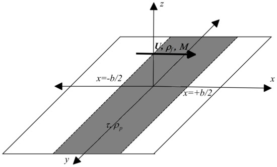
Figure 2.
Fluid and strip plate coupled system.
5. Rectangular Plate
Figure 3 shows a schematic of the second problem considered. Now, the plate also has a finite width 2d; the limit of this problem gives the first problem. Again using piston theory, the vibration equation takes the form
The plate was assumed to be simply supported at all sides, and thus, the boundary conditions are
Non-dimensionalization is similarly defined:
and again, getting rid of stars, the non-dimensional problem is
with the same and u as before. In this case, the solution was assumed to be in the following form:
This is the first term of a Fourier expansion in , but the common wisdom is that the higher terms do not affect the results [7,11]. The reason for this can be explained as follows: Like any other linear vibration problem, the flutter of a flat plate or strip will have mode shapes that depend on the mode numbers (basically, the numbering of the eigenvalues starting from the simplest mode). In the simplest case, the plate will vibrate like a single sinus wave, without changing the sign between its boundaries. The higher modes will have sign changes and nodes within the rectangular region. These higher modes will also have higher vibration frequencies. From a physical point of view, it is reasonable to expect that the plate will more easily vibrate in the shape of a simple sinus wave rather than a complicated shape with nodes and sign changes. Therefore, the leading sinus wave will exhibit unstable vibrations before any of the higher modes. Therefore, using (43), (40)–(42) become
The solution of (44) and (45) is carried out exactly as before, where only the expression changes.
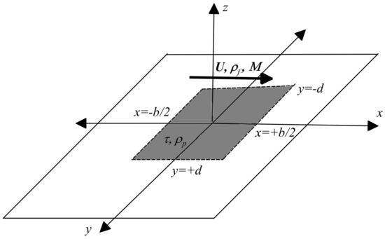
Figure 3.
Fluid and rectangular coupled system.
6. Analytical Solution
The solutions of both problems were found by the collocation method above. These problems can also be solved analytically, but the problem with the analytical solution is that the solution procedure involves finding the roots of a quartic equation and the resulting determinant involves transcendent functions and searching for their zeroes is difficult. The collocation method is simpler to apply and is similar to the analytical solution in terms of performance. The solutions of both (22) and (44) were sought in the form
Substituting (47) and (22) gives
and (44) gives
Denoting the roots of these equations as , , , and , the solutions can be written as
Applying the boundary conditions (23) and (45) both give
The difference between the two solutions is due to the fourth-degree algebraic Equations (48) and (49). For a non-trivial solution, the determinant of the coefficients in (51) should be zero.
This gives as a function of the other parameters in the problem. Although this is the analytical solution, the evaluation of the flutter velocity using this is quite difficult compared with the numerical collocation method. First, the evaluation of determinants is known to be numerically problematic, needing higher-precision computations. The second difficulty is the evaluation of the roots of the quartic equation. Although there is an exact formula for quartic equations, using numerical methods is advantageous here also.
7. Results and Discussion
Collocation solutions were found for , and 14 and sufficient convergence was observed for . Table 1 shows the convergence of the results for the flutter velocity while increasing the number of collocation points. The collocation points were chosen to be equally spaced for in all cases.

Table 1.
The convergence of the results while increasing the number of collocation points.
The solution of (48) (analytical solution) was found by an iterative shooting method [27,28,29]. Table 2 shows the comparisons between the collocation and analytical solutions.
Table 2.
Numerical results for a randomly chosen value of the two methods.
The collocation solution agreed with the analytical solution. To derive the solutions analytically, we used another method, the shooting method [27,29], which agreed with the collocation method solutions, as shown in Table 3. As mentioned, the collocation method gives results quickly; the analytical solution here is meant to check the correctness of the collocation solution. Another validation of the results is presented here by way of comparison with Dowell 1966, which shows similar results, bearing in mind that in the mentioned work, full potential theory was used, and the solution was carried out for an infinite plate in the direction of flow. The results obtained in this study for small d agreed with Dowell [7,25]. Although this is a theoretical study of flutter, a simple comparison with experiment was carried out. The type of experiment for the solution attempted here seems to be rare. The NACA Technical Note 3914 (1957) ([30]) lists some comparable measurements on thin panels. In that experimental study, some of the boundary conditions were also different. Furthermore, it was extremely difficult to experimentally imitate the plate boundary conditions. But, the magnitude of the numbers should give some idea about the validity of the theoretical solution. The notation and the system of units used were also different. But, after an adjustment, the following values for the experiment and the present computations were obtained.
Table 3.
Comparison of some results with NACA report ([30]).
Considering the differences in the setup and the difficulty in experimentally realizing the boundary conditions, it can be safely stated that the computations were in agreement with the experiment. For the cases of brass and aluminum, the computed flutter velocities were beyond the capabilities of the experiment. Therefore, it is natural that no flutter was observed.
7.1. Infinite Strip
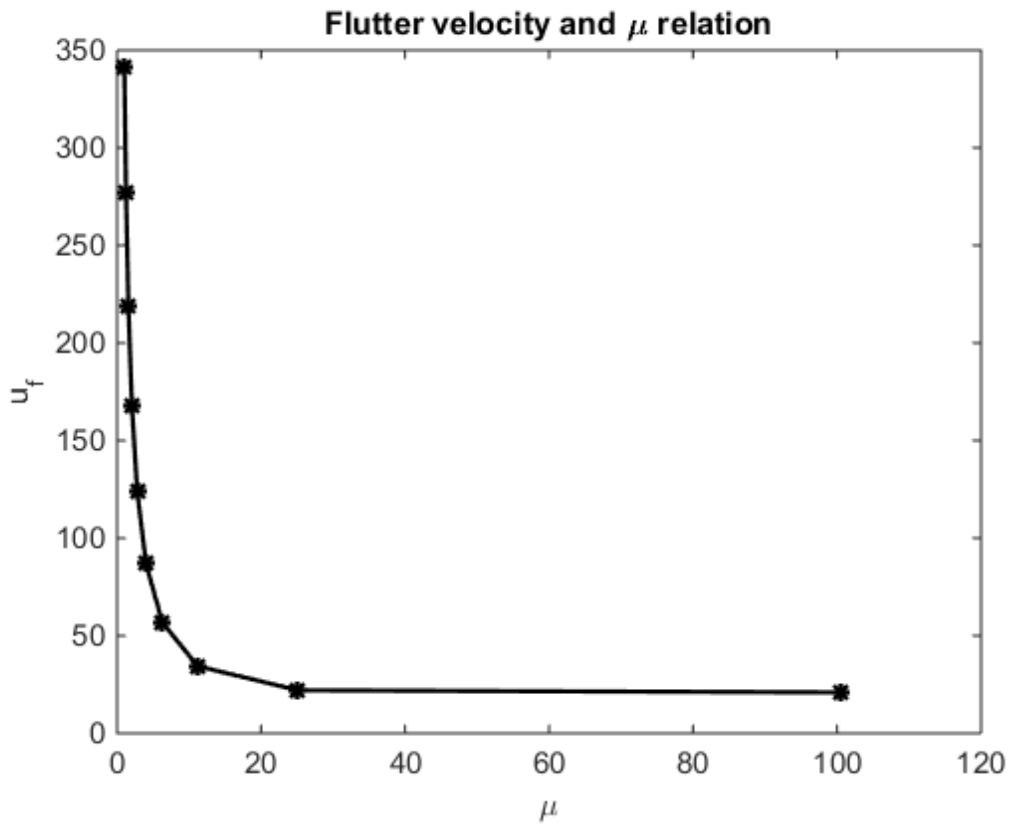
Figure 4 shows the non-dimensional flutter velocity as a function of the mass ratio. As expected, the flutter velocity decreased with increasing mass ratio. Since the curve in Figure 4 seems to have a simple structure, a mathematical expression between and could be developed by using curve fitting. This was done by using Matlab 2023b and the result was
This equation gives the same points as in Figure 4 within an error of 1 percent.

Figure 4.
Relationship between the non-dimensional mass ratio and the dimensionless flutter velocity for the strip plate given in Figure 1.
7.2. Rectangular Plate
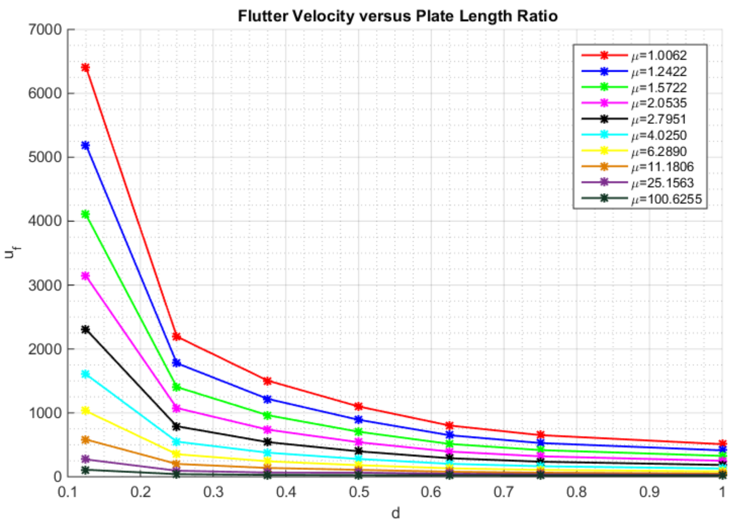
For a rectangular plate, there are two parameters that the flutter velocity depends on: the mass ratio and plate width ratio. Figure 5 shows the flutter velocity as a function of the plate width ratio for various values of the mass ratio for . The results for are shown in a separate Figure 5. It was observed that the flutter velocity decreased and asymptotically converged to the value for the infinite strip as the plate width increased.
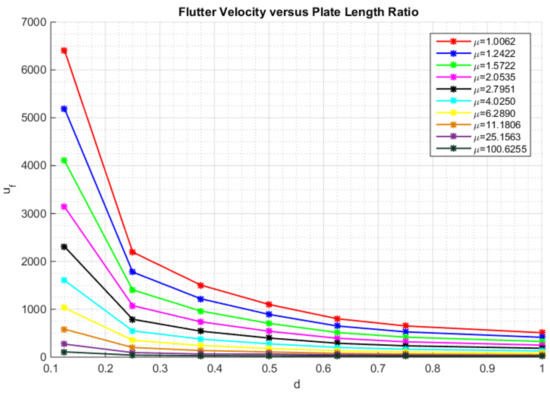
Figure 5.
Relation between u and d in different situations for the case .
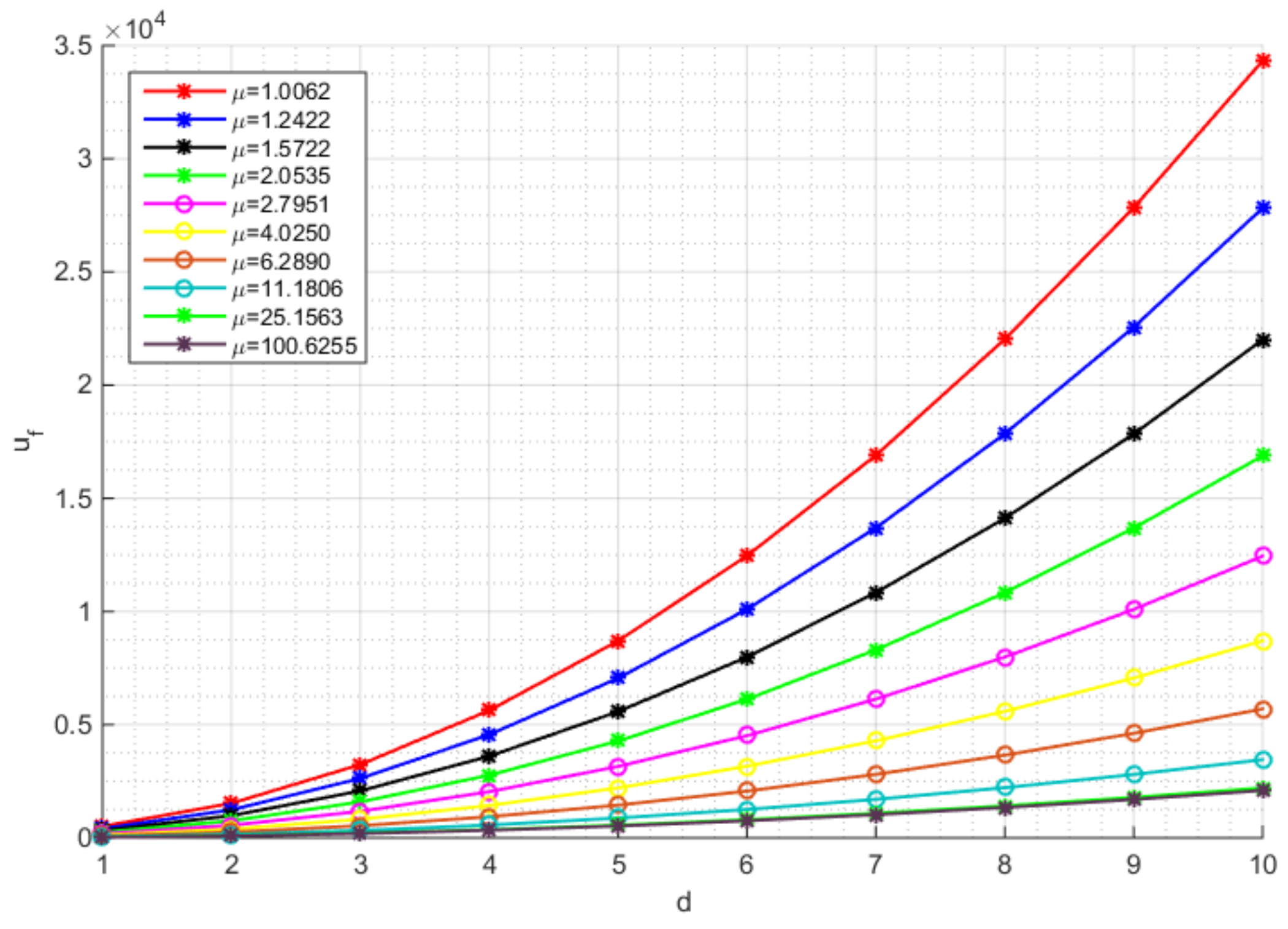
To generalize (53) to a rectangular plate, it was found to be useful to look at the graph of (Figure 6). We assumed the relationship between the flutter velocities for finite and infinite width plates to be
Here, is the expression (53), and by curve fitting, was found to be
Equation (54) gives the flutter velocity in Figure 6 within 1 percent for and . To give an example, for aluminum (with a density , elasticity modulus GPa, Poisson’s ratio ) plate of thickness 5 mm for m and m, (54) gave the non-dimensional flutter velocity as 91.7847 (91.166737 with the collocation method) and the actual flutter velocity was 704.5209 m/s (699.7770 m/s with the collocation method). With the use of (54), design engineers can easily and rapidly predict the flutter velocity. This is the main novelty of this paper, i.e., to predict the flutter velocity of a plate in different situations.
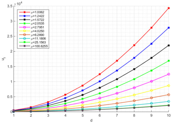
Figure 6.
Relationship between and d in different situations for the case .
8. Conclusions
To summarize, the flutter velocity of a plate structure under very varied geometric conditions can be estimated with the simple algebraic expressions given in this study. These expressions were derived by curve fitting to data obtained by the collocation method. To validate the collocation results, the analytical solution was also found and seen to give the same results. The novelty of the solution is the correlation between the flutter velocity and the other model parameters. In practice, these correlation equations should be very useful for design engineers in order to predict the flutter velocity. The range of the expressions given cover a very wide range of mass ratios (from 1 to 100) and a corresponding range of non-dimensional flutter velocities (from very low velocities up to about 6500).
Author Contributions
Conceptualization, A.S. (Aziz Sezgin), B.D., L.E.S. and E.U.; methodology, A.S. (Aziz Sezgin) and E.U.; software, A.S. (Alaattin Sayin), H.Y., H.O.O. and S.K.; validation, A.S. (Aziz Sezgin), B.D. and L.E.S.; formal analysis, H.O.O.; investigation, A.S. (Aziz Sezgin); resources, B.D. and S.K.; data curation, A.S. (Aziz Sezgin); writing—original draft preparation, A.S. (Aziz Sezgin) and E.U.; writing—review and editing, A.S. (Aziz Sezgin), B.D. and E.U.; visualization, H.O.O.; supervision, E.U.; project administration, A.S. (Aziz Sezgin), B.D. and E.U.; funding acquisition, All authors. All authors read and agreed to the published version of this manuscript.
Funding
This research received no external funding.
Institutional Review Board Statement
Not applicable.
Informed Consent Statement
Not applicable.
Data Availability Statement
The data presented in this study are available on request from the corresponding author.
Conflicts of Interest
The authors declare no conflicts of interest.
Abbreviations
| Symbol | Definition |
| E | Young’s modulus |
| Thickness of plate | |
| b | Length of plate |
| d | Width of plate |
| Density of plate | |
| w | Displacement of plate |
| Poisson’s ratio | |
| U | Velocity of the fluid |
| Density of the fluid | |
| M | Mach number |
| Mass ratio | |
| Dimensionless sound velocity | |
| Base function | |
| R | Residual |
| N | Number of collocation points |
| Dimensionless flutter velocity |
References
- Bisplinghoff, R.L.; Ashley, H.; Halfman, R.L. Aeroelasticity. In Dover Books on Aeronautical Engineering Series; Dover Publications: New York, NY, USA, 1996. [Google Scholar]
- Dowell, E.H.; Crawley, E.F.; Curtiss, H.C.; Peters, D.A.; Scanlan, R.H.; Sisto, F. A Modern Course in Aeroelasticity; Springer Science and Business Media: Dordrecht, The Netherlands, 1995. [Google Scholar]
- AGARD. Manual on Aeroelasticity; Report No: 578; NATO: Washington, DC, USA, 1971. [Google Scholar]
- Erol, U.; Sule, K. Vibrations of an Infinite Plate Placed in a Circular Channel Containing Fluid Flow. Aircr. Eng. Aerosp. Technol. 2010, 81, 533–535. [Google Scholar]
- Epureanu, B.I.; Yin, S.H. Identification of damage in an aeroelastic system based on attractor deformations. Comput. Struct. 2004, 82, 2743–2751. [Google Scholar] [CrossRef]
- Vedeneev, V.V. Panel flutter at low supersonic speeds. J. Fluids Struct. 2012, 29, 79–96. [Google Scholar] [CrossRef]
- Dowell, E.H. Flutter of infinitely Long Plates and Shells. Part 1: Plate. AIAA J. 1966, 4, 1370–1377. [Google Scholar] [CrossRef]
- Durak, B. Theoretical Investigation of Fluid-Elastic Body Interactions in Shell Structures. Ph.D. Thesis, Istanbul University, Istanbul, Türkiye, 2018. [Google Scholar]
- Kapkin, S.; Demir, M.S.; Kaya, M.O.; Uzal, E. Flutter of a Membrane in a Stagnation Flow. J. Appl. Fluid Mech. 2019, 12, 981–985. [Google Scholar] [CrossRef]
- Uzal, E.; Korbahti, B. Vibration control of an elastic strip by a singular force. Sadhana 2010, 35, 233–240. [Google Scholar] [CrossRef]
- Uzal, E.; Korbahti, B. Vibrations of an Anisotropic Plate Under Fluid Flow in a Channel. J. Vib. Control 2007, 13, 1191–1204. [Google Scholar]
- Sezgin, A.; Krstic, M. Boundary Backstepping Control of Flow-Induced Vibrations of a Membrane at High Mach Numbers. J. Dyn. Syst. Meas. Control 2015, 137, 081003-1. [Google Scholar] [CrossRef]
- Tubaldi, E.; Alijani, F.; Amabili, M. Non-linear vibrations and stability of a periodically supported rectangular plate in axial flow. Int. J. Non-Linear Mech. 2014, 66, 54–65. [Google Scholar] [CrossRef]
- Li, W.L. Vibration analysis of rectangular plates with general elastic boundary supports. J. Sound Vib. 2018, 422, 15–33. [Google Scholar] [CrossRef]
- Lin, T.R.; Zhang, K. An analytical study of the free and forced vibration response of a ribbed plate with free boundary conditions. J. Sound Vib. 2004, 273, 619–635. [Google Scholar] [CrossRef]
- Liu, C.; Xie, C.; Meng, Y.; Bai, L. Experimental and Numerical Flutter Analysis Using Local Piston Theory with Viscous Correction. Aerospace 2023, 10, 870. [Google Scholar] [CrossRef]
- Ashley, H.; Zartarian, G. Piston Theory-A New Aerodynamic Tool for the Aeroelastician. J. Aeronaut. Sci. 1956, 23, 1109–1118. [Google Scholar] [CrossRef]
- Eisenberger, M.; Deutsch, A. Solution of thin rectangular plate vibrations for all combinations of boundary conditions. J. Sound Vib. 2019, 452, 1–12. [Google Scholar] [CrossRef]
- Shitov, S.; Vedeneev, V. Flutter of rectangular simply supported plates at low supersonic speeds. J. Fluids Struct. 2017, 69, 154–173. [Google Scholar] [CrossRef]
- Vedeneev, V. Flutter of a Wide Strip Plate in a Supersonic Gas Flow. Fluid Dyn. 2005, 40, 805–817. [Google Scholar] [CrossRef]
- Yao, G.; Liu, D. Aeroelastic stability analysis of a pyrotechnic separation plate in subsonic airflow. Appl. Math. Model. 2022, 107, 574–590. [Google Scholar] [CrossRef]
- Tang, D.; Dowell, E.H. Limit cycle oscillations of two-dimensional panels in low subsonic flow. Int. J. Non-Linear Mech. 2002, 37, 1199–1209. [Google Scholar] [CrossRef]
- Cho, D.S.; Kim, B.H.; Kim, J.H.; Vladimir, N.; Choi, T.M. Forced vibration analysis of arbitrarily constrained rectangular plates and stiffened panels using the assumed mode method. Thin-Walled Struct. 2015, 90, 182–190. [Google Scholar] [CrossRef]
- Tenenbaum, J.; Eisenberger, M. Analytic solution of rectangular plate buckling with rotationally restrained and free edges. Thin-Walled Struct. 2020, 157, 106979. [Google Scholar] [CrossRef]
- Dowell, E.H.; Hall, K.C. Modeling of Fluid-Structure Iteration. Annu. Rev. Fluid Mech. 2001, 33, 445–490. [Google Scholar] [CrossRef]
- Bortoli, A.L.D. Aeroelastic analysis of panels in compressible flows. J. Fluids Struct. 2005, 20, 189–195. [Google Scholar] [CrossRef]
- Morrison, D.D.; Riley, J.D.; Zancanaro, J.F. Multiple shooting method for two-point boundary value problems. Commun. ACM 1962, 5, 613–614. [Google Scholar] [CrossRef]
- Osborne, M.R. On shooting methods for boundary value problems. J. Math. Anal. Appl. 1969, 27, 417–433. [Google Scholar] [CrossRef]
- Fang, L.; Vandewalle, S.; Meyers, J. An SQP-based multiple shooting algorithm for large-scale PDE-constrained optimal control problems. J. Comput. Phys. 2023, 477, 111927. [Google Scholar] [CrossRef]
- Sylvester, M.A.; Baker, B.E. Some Experimental Studies of Panle Flutter at Mach Number 1.3; National Advisory Committee for Aeronautics Technical Note; NACA TN 3914; NACA: Washington, DC, USA, 1957; Volume 3914. [Google Scholar]


Disclaimer/Publisher’s Note: The statements, opinions and data contained in all publications are solely those of the individual author(s) and contributor(s) and not of MDPI and/or the editor(s). MDPI and/or the editor(s) disclaim responsibility for any injury to people or property resulting from any ideas, methods, instructions or products referred to in the content. |
© 2024 by the authors. Licensee MDPI, Basel, Switzerland. This article is an open access article distributed under the terms and conditions of the Creative Commons Attribution (CC BY) license (https://creativecommons.org/licenses/by/4.0/).