Solar Sail-Based Mars-Synchronous Displaced Orbits for Remote Sensing Applications

Abstract

A solar sail is a propellantless propulsion system that allows a spacecraft to use solar radiation pressure as a propulsive source for planetary and deep space missions that would be difficult, or even unfeasible, to accomplish with more conventional thrusters, either chemical or electric. A challenging application for these fascinating propulsion systems is a heliocentric mission that requires a displaced non-Keplerian orbit (DNKO), that is, a solar sail-induced closed trajectory in which the orbital plane does not contain the Sun’s center of mass. In fact, thanks to the pioneering work of McInnes, it is known that a solar sail is able to reach and maintain a family of heliocentric DNKOs of given characteristics. The aim of this paper is to analyze the properties of Mars-synchronous circular DNKOs, which have an orbital period matching that of the planet for remote sensing applications. In fact, those specific displaced orbits allow a scientific probe to continuously observe the high-latitude regions of Mars from a quasi-stationary position relative to the planet. In this context, this paper also analyzes the optimal (i.e., the minimum-time) heliocentric transfer trajectory from the Earth to circular DNKOs in two special mission scenarios taken as a reference.

1. Introduction

Solar radiation pressure is the physical phenomenon that enables the operation of solar sails, a class of advanced propulsion systems for space navigation that convert sunlight into propulsive acceleration without the need for propellant expenditure [1,2,3]. In particular, photonic solar sails reflect photons coming from the Sun thanks to a large and thin membrane coated with a highly reflective material (e.g., aluminum), while refractive [4,5] and diffractive [6,7,8] sails exploit other optical phenomena such as refraction and diffraction of light. Thanks to their intrinsic nature as propellantless propulsion systems, solar sails are particularly suitable for carrying out long-term missions or covering trajectories that require the continuous application of a steerable (but usually of small magnitude) thrust [9].

A category of heliocentric missions to which solar sails would be well suited is that constituted by the generation and maintenance of displaced non-Keplerian orbits (DNKOs) around the Sun [10]. They are two-dimensional, closed heliocentric trajectories that do not contain the center of mass of the primary attractor of the solar sail itself [11,12] (i.e., the Sun) and, for this reason, require a continuous propulsive acceleration to balance both the (apparent) centrifugal and gravitational forces acting on the spacecraft. In this context, it is interesting to recall that an approximation of a circular or an elliptical DNKO may also be obtained by considering a sequence of Keplerian arcs patched by a set of suitable (high-thrust-induced) impulsive maneuvers, as proposed first by McInnes [13] for a circular orbit and then generalized by Caruso et al. [14] for a generic, elliptic trajectory.

The employment of a heliocentric DNKO is useful for monitoring high-latitude regions of planets [15] (or generic celestial bodies) and it is an interesting potential option for many other mission applications, as discussed by McInnes at p. 25 of Ref. [16] and by McKay et al. [10] in their useful and interesting survey paper published in 2011. Among all the possible scientific applications, it is interesting to mention, for example, continuous solar wind monitoring [17,18], real-time polar imaging and stereographic investigations of a planetary surface [19,20,21], continuous communications with high-latitude regions, and in situ observations of the planetary rings. That is the reason why so many studies have dealt with the problem of reaching and maintaining DNKOs by means of a solar sail-propelled spacecraft. In this context, Bookless and McInnes [12] proposed exploiting solar sails to generate families of artificial libration points and displaced (periodic) orbits around the Earth, while Gong et al. [19,22] analyzed the possibility of maintaining elliptical DNKOs by means of a solar sail for planetary polar observation. In particular, Refs. [19,22] investigated the relative orbit design and control methods for formation flight around an assigned displaced orbit maintained by a spacecraft equipped with a classical (photonic) solar sail. About ten years ago, Song et al. [21] analyzed solar sail displaced orbits in Hill’s restricted three-body problem, while Ceriotti et al. [23,24] investigated the interesting concept of a pole-sitter mission, in which the spacecraft is always above one of Earth’s geographic poles to obtain the continuous observation of planetary high-latitude regions. Finally, Heiligers et al. [25] analyzed the possibility of using a classical solar sail to generate artificial equilibrium points and displaced periodic orbits around small bodies in the solar system such as asteroids or binary asteroid systems. More recently, Bassetto et al. [26,27] studied the performance of Zubrin’s magnetic sails [28,29,30] and Swartzlander’s diffractive sails [6,7,8] in maintaining circular DNKOs of assigned characteristics, with applications in a typical Earth-based mission scenario. From the point of view of the spacecraft dynamics along a DNKO, station keeping has also been studied in the context of three-body problem periodic orbits, which also suffer from deviations from nominal periodic behavior due to unmodeled physics. In this respect, the interested reader can refer to Refs. [31,32,33].

In this paper, a scientific interplanetary probe equipped with a photonic solar sail is required to trace a circular DNKO at an angular velocity equal to the mean motion of Mars [16] so as to maintain a constant average phase shift with respect to the angular position of the Red Planet along its heliocentric orbit. As part of Mars exploration missions, it is worth mentioning the work of MacDonald et al. [34], who proposed an Earth-Mars interplanetary communication relay in support of crewed missions to Mars. In fact, a Mars-synchronous DNKO, with its revolution period matching that of Mars, would be useful for remote sensing applications, allowing a scientific payload to continuously observe the high-latitude regions of Mars from a quasi-stationary position relative to the planet. Such a vantage point would offer unique possibilities to better understand some physical phenomena of great scientific interest that are specific to high-latitude areas, such as the existence of polygonal features, the occurrence of dust activities in the southern high-latitude regions, the mechanism capable of generating the lobate features located at high latitudes, or the origin of global-scale oscillations possibly due to waves in the atmosphere. Analogous to what has been recently discussed by the authors in Ref. [35], this paper also analyzes the rapid transfer trajectory from Earth to an assigned Mars-based DNKO as a function of typical solar sail performance characteristics, which are selected consistently with the propulsive requirements necessary for maintaining the target DNKO. In particular, the mission scenario is studied by neglecting the uncertainties related to both the solar sail optical parameters and the solar irradiance fluctuations [36,37,38].

This paper is structured as follows. Section 2 deals with the mathematical preliminaries. In particular, it first recovers the well-known thrust vector model of an ideal solar sail, that is, a flat solar sail with a perfectly reflecting coating, and then details the sail performance required to maintain a circular DNKO of given characteristics. Section 3 graphically illustrates the results previously presented and provides the distance of the spacecraft from Mars as a function of a set of design parameters. Section 4 addresses the transfer problem from the Earth to the circular DNKO, which is solved in an optimal framework by minimizing the total flight time, and shows the simulation results in two special scenarios taken as references. The final section contains the concluding remarks.

2. Mathematical Preliminaries

In this section, we summarize the mathematical model for describing both the solar sail-induced thrust vector and the propulsion system performance required to maintain a heliocentric DNKO of assigned characteristics. The interested reader may find a more exhaustive discussion about the arguments treated in this section by referring to McInnes’s fundamental textbook on solar sailing [16] or to Wright’s book [39].

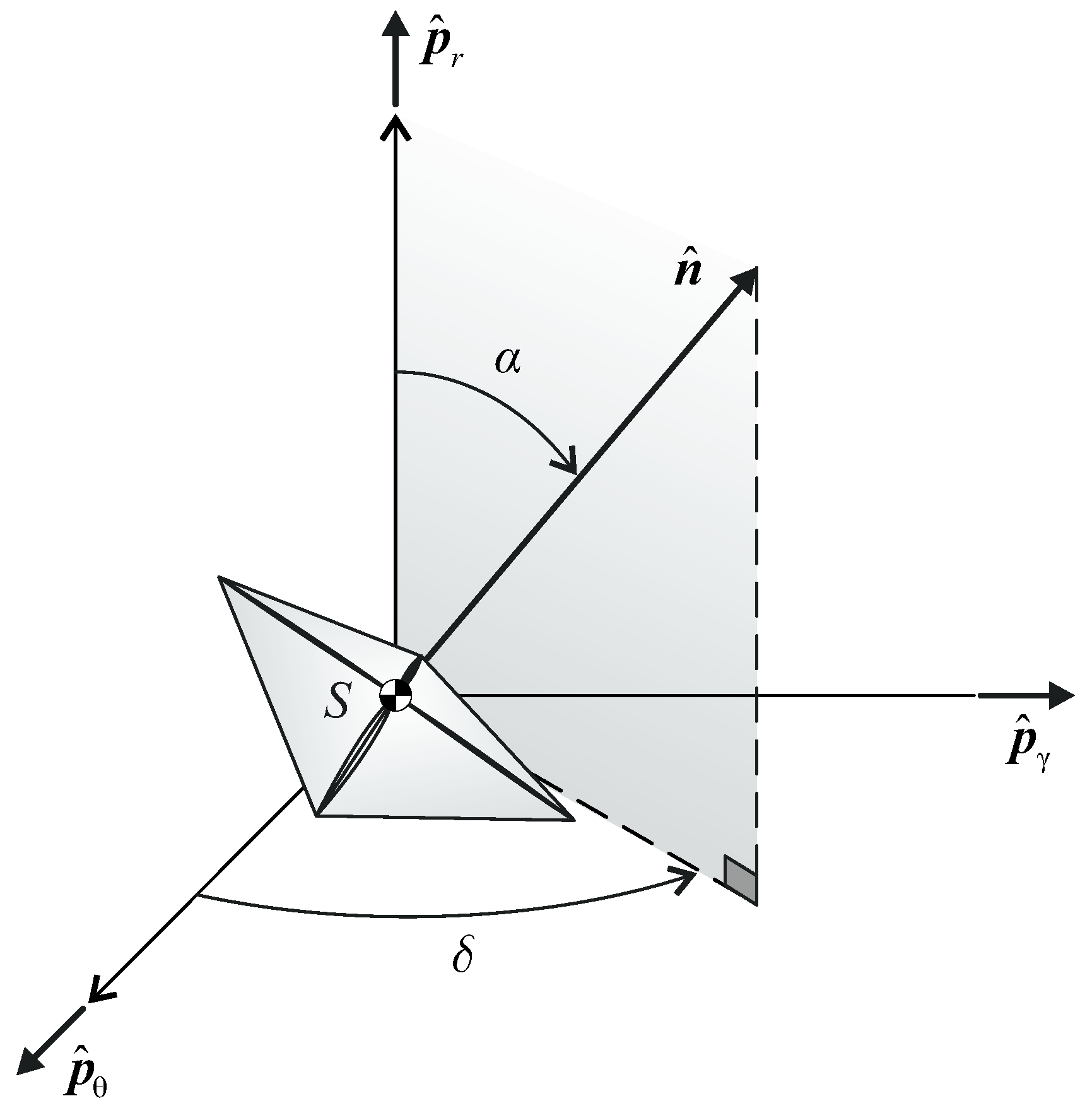
2.1. Thrust Vector Model of an Ideal Solar Sail

The propulsive acceleration vector provided by an ideal (i.e., flat and perfectly reflecting) solar sail depends on its attitude relative to the Sun [16,39]. In particular, when the degradation effects due to the space environment are neglected [40,41,42], the propulsive acceleration vector ${\mathit{a}}_p$ can be written as

$${\mathit{a}}_p=\beta {\displaystyle \frac{{\mu }_{\odot }}{r^2}}{cos}^2\alpha \widehat{\mathit{n}}$$

(1)

where $\beta$ is the lightness number, that is, the ratio of the maximum propulsive acceleration magnitude at a given distance from the Sun to the local magnitude of gravitational acceleration; ${\mu }_{\odot }\simeq 1.3271\times {10}^{11}{\mathrm{km}}^3/{\mathrm{s}}^2$ is the Sun’s gravitational parameter; r is the Sun-spacecraft distance; $\widehat{\mathit{n}}$ is the unit vector normal to the sail plane pointing outward from the Sun; and $\alpha \in [0,\pi /2]\mathrm{rad}$ is the sail cone angle, that is, the angle between the Sun-spacecraft line and the direction of $\widehat{\mathit{n}}$.

In particular, the lightness number $\beta$ is the typical performance parameter of an ideal solar sail and can be written as

$$\beta \triangleq {\displaystyle \frac{2I_{\oplus }A{r}_{\oplus }^2}{mc{\mu }_{\odot }}}$$

(2)

where $I_{\oplus }\simeq 1360.8\mathrm{W}/{\mathrm{m}}^2$ is the solar constant (i.e., the solar irradiance at the reference distance $r_{\oplus }\triangleq 1\mathrm{au}$ from the Sun), A is the surface area of the sail, m is the total mass of the spacecraft (assumed to be constant), and c is the speed of light in vacuum. From Equation (2), it turns out that, basically, the sail lightness number is inversely proportional to the sail loading $m/A$, defined as the ratio of the spacecraft mass to the sail exposed area [16,39].

2.2. Sail Performance Required to Maintain a Circular DNKO

Consider a heliocentric mission scenario in which a solar sail-based spacecraft traces a DNKO designed to obtain continuous observation of Mars high-latitude regions.

With reference to the scheme in Figure 1, we introduce a perifocal reference system ${\mathcal{T}}_O(O;p,q,w)$, where O is the center of mass of the Sun, axis p is aligned with the eccentricity vector of Mars heliocentric orbit (omitted in the figure for simplicity), and axis w is parallel to the angular momentum of Mars orbit. Therefore, the plane $(p,q)$ coincides with the orbital plane of Mars in its motion around the Sun.

The heliocentric DNKO to be maintained is a circular trajectory of constant radius $\rho$, which is centered on the point $O^{\prime }$ belonging to axis w; see Figure 1. The plane of the displaced orbit (i.e., the green disk in the previous figure) is parallel to the orbital plane of Mars (i.e., the gray disk in the figure), and the distance between the two planes is denoted by H, which is positive (or negative) if $O^{\prime }$ belongs to the positive (or negative) semiaxis w. Furthermore, the solar sail-based spacecraft travels along the circular DNKO at a constant angular velocity $\omega$, which corresponds to the mean motion of Mars around the Sun, that is, $\omega \triangleq \sqrt{{\mu }_{\odot }/a^3}\simeq 0.5240\mathrm{deg}/\mathrm{day}$, where $a\simeq 1.5237\mathrm{au}$ is the semimajor axis of Mars heliocentric orbit.

In this way, the period of revolution of the spacecraft matches that of Mars, thus allowing remote sensing applications of the high-latitude regions of the Red Planet to be carried out. For an assigned value of angular velocity $\omega$, a circular DNKO may also be equivalently characterized by the elevation angle $\gamma$, that is, the angle between the Sun-spacecraft line and the orbital plane of Mars, and the Sun-spacecraft distance r, as it is sketched in Figure 1. Note that the conversion from the pair $\{r,\gamma \}$ to the pair $\{\rho ,H\}$ is given by the two simple equations

$$\rho =rcos\gamma ,H=rsin\gamma$$

(3)

while the reverse conversion is given by

$$r=\sqrt{{\rho }^2+H^2},\gamma =arctan\left({\displaystyle \frac{H}{\rho }}\right)$$

(4)

The heliocentric motion of the solar sail-based spacecraft is analyzed in a spherical reference frame ${\mathcal{T}}_S(O;r,\theta ,\gamma )$, with the origin S in the spacecraft center of mass and unit vectors $\{{\widehat{\mathit{p}}}_r,{\widehat{\mathit{p}}}_{\theta },{\widehat{\mathit{p}}}_{\gamma }\}$ defined as

$${\widehat{\mathit{p}}}_r\triangleq {\displaystyle \frac{\mathit{r}}{r}},{\widehat{\mathit{p}}}_{\theta }\triangleq {\displaystyle \frac{\widehat{\mathit{k}}\times \widehat{\mathit{r}}}{\parallel \widehat{\mathit{k}}\times \widehat{\mathit{r}}\parallel }},{\widehat{\mathit{p}}}_{\gamma }\triangleq {\widehat{\mathit{p}}}_r\times {\widehat{\mathit{p}}}_{\theta }$$

(5)

where $\mathit{r}$ is the Sun-spacecraft position vector and $\widehat{\mathit{k}}$ is the unit vector of Mars orbital angular momentum, that is, the direction of $\widehat{\mathit{k}}$ is perpendicular to the orbital plane of Mars. In particular, the position of the spacecraft is determined by three parameters, namely, the radial distance r, the azimuthal angle $\theta \in [0,2\pi )\mathrm{rad}$, and the elevation angle $\gamma \in [-\pi /2,\pi /2]\mathrm{rad}$. With reference to Figure 2, $\theta$ is the angle (measured counterclockwise) between p and the projection of vector $\mathit{r}$ onto the $(p,q)$ plane, while $\gamma$ is the angle between the direction of $\mathit{r}$ and the $(p,q)$ plane. Note that the sign of $\gamma$ corresponds to the (conventional) sign of the DNKO displacement H; compare Figure 1 and Figure 2.

As better detailed in Section 3.1, the solar sail-based spacecraft is outside the sphere of influence (SOI) of Mars and, therefore, the perturbative effect of the planet can be neglected [43]. Following the method detailed in [16] and looking at the scheme in Figure 3, the balance between propulsive, gravitational, and centrifugal accelerations acting on the spacecraft results in the following two scalar equations

$$\begin{array}{cc}\hfill & \beta {\displaystyle \frac{{\mu }_{\odot }}{r^2}}{cos}^2\alpha sin\alpha =\rho {\omega }^{2}sin\gamma \hfill \end{array}$$

(6)

$$\begin{array}{cc}\hfill & \beta {\displaystyle \frac{{\mu }_{\odot }}{r^2}}{cos}^3\alpha +\rho {\omega }^{2}cos\gamma ={\displaystyle \frac{{\mu }_{\odot }}{r^2}}\hfill \end{array}$$

(7)

which describe the spacecraft equilibrium in a rotating reference frame along ${\widehat{\mathit{p}}}_r$ and ${\widehat{\mathit{p}}}_{\gamma }$, respectively.

Now, by substituting Equation (6) into Equation (7) and using Equations (3) and (4), one obtains the following analytical result, which expresses the sail cone angle $\alpha$ as a function of the triplet $\{\rho ,H,r\}$, viz.

$$\alpha =arctan\left({\displaystyle \frac{\rho Hr}{a^3-r{\rho }^2}}\right)$$

(8)

while the required lightness number $\beta$ is obtained from Equation (6) by using Equations (3) and (4). In that case, the result is

$$\beta ={\displaystyle \frac{1-r{\rho }^2/a^3}{{cos}^3\alpha }}$$

(9)

where $\alpha$ is given by Equation (8). Note that changing the sign of H (or, equivalently, of $\gamma$) does not produce any change in the value of the required lightness number $\beta$, while it causes the cone angle to change its sign. Therefore, by virtue of this symmetry, only the results relating to positive $\gamma$ values are shown in the rest of this paper. The previous analytical results can be considered as a specific application to a Mars-based mission scenario of the general mathematical model discussed in [16].

3. Numerical Results

Using the mathematical model described in the previous section, the performance required by the ideal solar sail is evaluated as a function of the desired characteristics of the heliocentric, circular DNKO. In this context, Figure 4 shows the required values of $\{\alpha ,\beta \}$ as a function of $\{\rho /a,H/a\}$.

In particular, Figure 4a is consistent with a low-performance solar sail (i.e., $\beta \le 0.05$), while Figure 4b is consistent with a medium/high-performance solar sail (i.e., $\beta \ge 0.05$). For comparison with the performance of actually designed solar sails, the obtained lightness number is just under $0.01$ for the LightSail 2 [44] (i.e., $\beta \simeq 0.0098$), Near-Earth Asteroid Scout (NEA Scout) [45,46] (i.e., $\beta \simeq 0.0093$), and Advanced Composite Solar Sail System (ACS3) [47] (i.e., $\beta \simeq 0.0077$) missions. Therefore, based on the classification made in this paper, the aforementioned first-generation missions fall in the group of low-performance solar sails.

Note that the gray areas in Figure 4 correspond to the envelope of all the spheres of influence of Mars during its revolution around the Sun. In fact, the SOI of Mars is a spherical region that moves in the interplanetary space following the Red Planet and with a variable radius depending on the Sun-Mars distance. We can indeed express the radius $R_{\mathrm{SOI}}$ of Mars SOI as

$$R_{\mathrm{SOI}}={\rho }_{♂}{\left({\displaystyle \frac{{\mu }_{♂}}{{\mu }_{\odot }}}\right)}^{2/5}$$

(10)

where ${\mu }_{♂}\simeq \mathrm{42,828}{\mathrm{km}}^3/{\mathrm{s}}^2$ represents the gravitational parameter of Mars and

$${\rho }_{♂}={\displaystyle \frac{a\left(1-e^2\right)}{1+ecos\nu }}$$

(11)

is the Sun-Mars distance, ranging from a minimum of $1.3814\mathrm{au}$ to a maximum of $1.6660\mathrm{au}$, as a function of the planet true anomaly $\nu$ (i.e., the angle between axis p and the current Sun-Mars line).

For example, consider the two scenarios indicated in Figure 5. In particular, scenario A is obtained with $\rho =0.998840a$ and $H=0.01a$ (from which $\beta \simeq 0.1$), while scenario B is obtained with $\rho =0.999423a$ and $H=0.005a$ (from which $\beta \simeq 0.05$). Note that $\alpha \simeq 71\mathrm{deg}$ in both cases. These two possible cases (the former consistent with a high-performance solar sail and the latter with a medium-performance solar sail) are used as examples in the next sections.

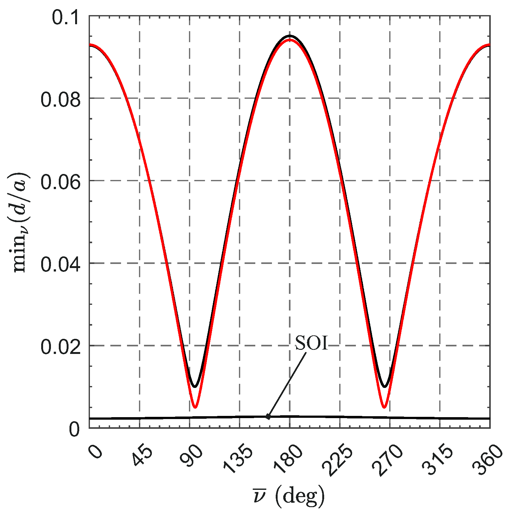
3.1. Evaluation of the Mars-Spacecraft Distance

The effectiveness of a scientific mission to monitor the high-latitude regions of Mars depends on the distance d of the spacecraft from the planet; see the scheme in Figure 1. Note that the monitoring of Mars polar region can be also obtained with a Keplerian orbit with a suitable inclination. However, in that case, the observation of the high-latitude regions of the planet is carried out only in a part of the spacecraft (planetocentric) orbit, while a DNKO ensures continuous monitoring. By replicating the procedure described in Ref. [27], in this section we quantify the Mars-spacecraft distance, showing that it depends on four parameters, namely, the DNKO radius $\rho$, the DNKO displacement H, the true anomaly $\nu$ of Mars, and the point in the planetary orbit (described by the angle $\overline{\nu }$) at which the spacecraft and Mars have the same angular position in their (always parallel) planes of motion.

For this purpose, consider the components of the Sun-spacecraft position vector $\mathit{r}$ in the spherical reference frame ${\mathcal{T}}_O$, that is

$${\left[\mathit{r}\right]}_{{\mathcal{T}}_O}=\left[\begin{array}{c}\rho cos\theta \\ \rho sin\theta \\ H\end{array}\right]$$

(12)

where $\theta$ is the angle between the projection of $\mathit{r}$ into the orbital plane of Mars and axis p, as it is sketched in Figure 1 and Figure 2. The components of the Sun-Mars position vector in ${\mathcal{T}}_O$, instead, are given by

$${\left[{\mathit{r}}_{♂}\right]}_{{\mathcal{T}}_O}=\left[\begin{array}{c}{\rho }_{♂}cos\nu \\ {\rho }_{♂}sin\nu \\ 0\end{array}\right]$$

(13)

where ${\rho }_{♂}$ is given by Equation (11). In particular, the value of $\theta$ may also be written as

$$\theta =\omega \left(t-t_0\right)+{\theta }_0$$

(14)

where t is the time and ${\theta }_0$ is the angular offset between the spacecraft and axis p at the initial time $t_0\triangleq 0$. The latter is here defined, without loss of generality, as the time instant at which Mars passes the perihelion (i.e., $\nu \left(t_0\right)\triangleq 0$), from which it follows that ${\theta }_0$ also describes the angular offset between the spacecraft and Mars at the reference time $t_0$. Therefore, for net of multiples of one period of revolution of Mars (corresponding to about $687\mathrm{days}$), the time t can be written as a function of $\nu$ as

$$t=\sqrt{{\displaystyle \frac{a^3}{{\mu }_{\odot }}}}\left(E-esinE\right)$$

(15)

where $E\in [0,2\pi )\mathrm{rad}$ is the eccentric anomaly of Mars, given by the well-known formula

$$E\triangleq 2arctan\left(\sqrt{{\displaystyle \frac{1-e}{1+e}}}tan{\displaystyle \frac{\nu }{2}}\right)$$

(16)

The value of ${\theta }_0$ may be determined backward from the value of $\nu$ (namely, $\overline{\nu }$) such that $\theta =\overline{\nu }$, that is, the value of $\nu$ (assumed to exist) at which the solar sail and Mars have the same angular position in their planes of motion around the Sun. Accordingly, the value of E when $\nu =\overline{\nu }$ is given by

$$\overline{E}=2arctan\left(\sqrt{{\displaystyle \frac{1-e}{1+e}}}tan{\displaystyle \frac{\overline{\nu }}{2}}\right)$$

(17)

the corresponding time instant is

$$\overline{t}=\sqrt{{\displaystyle \frac{a^3}{{\mu }_{\odot }}}}\left(\overline{E}-esin\overline{E}\right)$$

(18)

while ${\theta }_0$ is given by

$${\theta }_0=\overline{\nu }-\omega \overline{t}$$

(19)

Bearing in mind that $\overline{t}=\overline{t}\left(\overline{\nu }\right)$ (see Equations (17) and (18)), then Equation (19) gives ${\theta }_0={\theta }_0\left(\overline{\nu }\right)$, which is plotted in Figure 6. Note that $|{\theta }_0|$ is maximum when $\overline{\nu }\simeq \{94.02,265.98\}\mathrm{deg}$ and its value is about $10.71\mathrm{deg}$. Accordingly, the angular offset between the spacecraft and Mars, defined as

$$\varphi \triangleq \theta -\nu =\omega \left(t-\overline{t}\right)-\left(\nu -\overline{\nu }\right)$$

(20)

is an explicit function of $\{\nu ,\overline{\nu }\}$ according to Equations (15)–(18), so it changes throughout the period of revolution of Mars. However, as already shown in [27], its mean integral value with respect to $\nu$, that is, the function

$$\Phi \triangleq {\displaystyle \frac{1}{2\pi }}{\int }_0^{2\pi }\varphi \mathrm{d}\nu \equiv {\theta }_0$$

(21)

turns out to coincide with the angular displacement between the solar sail-based spacecraft and Mars when the latter passes the perihelion.

The distance d between the spacecraft and the center of mass of Mars, given by

$$d=\sqrt{{\left({\rho }_{♂}cos\nu -\rho cos\theta \right)}^2+{\left({\rho }_{♂}sin\nu -\rho sin\theta \right)}^2+H^2}$$

(22)

is an explicit function of $\{\rho ,H,\nu ,\overline{\nu }\}$ and is represented (normalized with respect to a) in Figure 7 for $H=0.005a$. In particular, $\rho /a$ ranges between $\left(1-e\right)\simeq 0.9066$ (which corresponds to the perihelion of Mars orbit) and the maximum value that ensures a feasible (i.e., positive) value of $\beta$. This last condition holds if $r{\rho }^2<a^3$; see also Equation (9).

Figure 8, instead, shows the variation of $d/a$ as a function of $\{\nu ,\overline{\nu }\}$ in the scenario A. The corresponding figure for scenario B is substantially coincident with Figure 8 and has been omitted. Note that Figure 8 also displays the radius of Mars SOI, which is given by Equations (10) and (11) as a function of $\nu$. Finally, Figure 9 shows the variation of ${min}_{\nu }(d/a)$ with $\overline{\nu }$ for scenarios A and B.

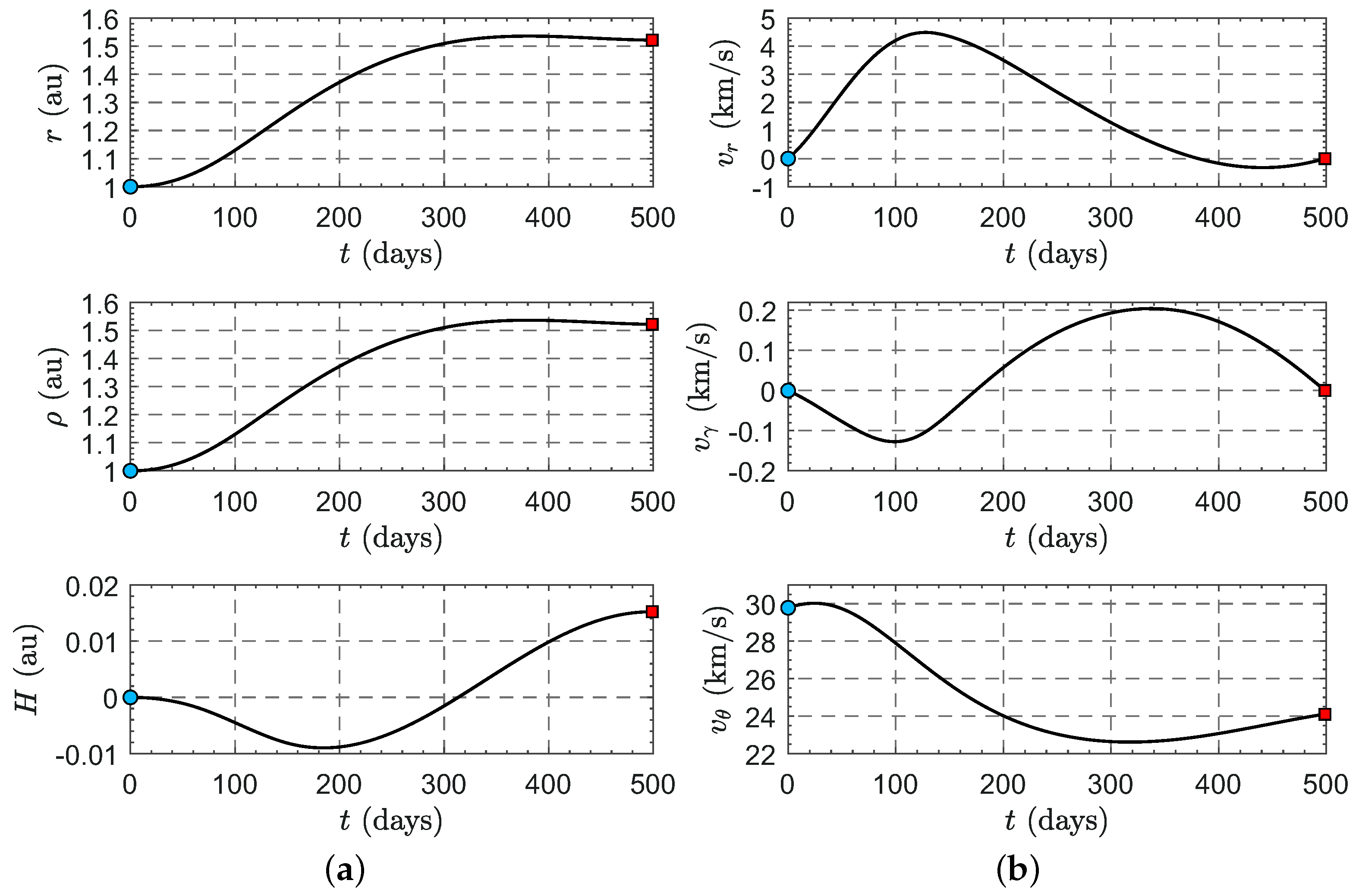
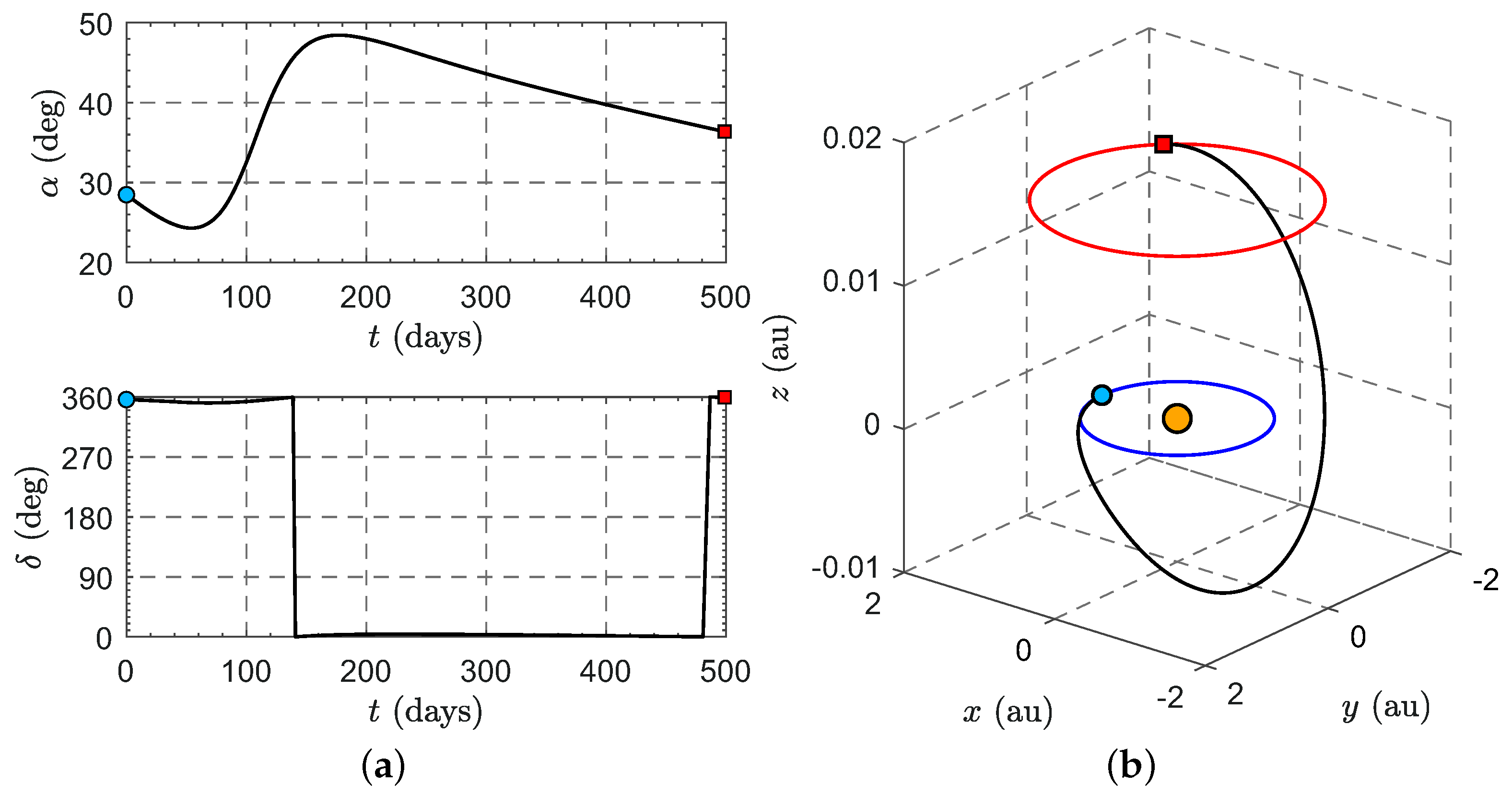
4. Preliminary Study of the Heliocentric Transfer Trajectory

The problem of the heliocentric transfer from Earth to the target DNKO is addressed in this section with the simplifying hypotheses that the solar sail-based spacecraft starts from a circular orbit of radius $r_{\oplus }=1\mathrm{au}$ and that the plane of motion of the starting orbit is coplanar to the orbit of Mars, that is, to the $(p,q)$ plane; see the scheme in Figure 1. These two assumptions, in fact, allow both the dynamic model and the optimal control law adopted in [35] to be retrieved while appropriately changing the boundary conditions. Note that these two simplifying hypotheses are reasonable since the orbital plane of Mars is slightly inclined with respect to the ecliptic plane (i.e., about $1.85\mathrm{deg}$) and the eccentricity of Earth’s orbit is very small (i.e., about $0.0167$). Practically, such a situation may be achieved by launching the spacecraft at the moment in which the Earth’s orbit intersects the orbital plane of Mars and giving it a velocity change (which is of the order of $1\mathrm{km}/\mathrm{s}$) to make the required orbital plane change in addition to the velocity change necessary to escape from the gravitational field of Earth. During the (interplanetary) transfer phase of the mission, the spacecraft uses the solar sail-induced propulsive acceleration to reach the target DNKO. In this respect, the sail propulsive characteristics are the same required to maintain the target DNKO.

According to Ref. [48], the (heliocentric) equations of motion of a spacecraft in the spherical reference frame are

$$\begin{array}{cc}\hfill \dot{r}& =v_r\hfill \end{array}$$

(23)

$$\begin{array}{cc}\hfill \dot{\theta }& ={\displaystyle \frac{v_{\theta }}{rcos\gamma }}\hfill \end{array}$$

(24)

$$\begin{array}{cc}\hfill \dot{\gamma }& ={\displaystyle \frac{v_{\gamma }}{r}}\hfill \end{array}$$

(25)

$$\begin{array}{cc}\hfill {\dot{v}}_r& ={\displaystyle \frac{v_{\theta }^2+v_{\gamma }^2}{r}}-{\displaystyle \frac{{\mu }_{\odot }}{r^2}}+a_r\hfill \end{array}$$

(26)

$$\begin{array}{cc}\hfill {\dot{v}}_{\theta }& ={\displaystyle \frac{v_{\theta }{v}_{\gamma }tan\gamma -v_r{v}_{\theta }}{r}}+a_{\theta }\hfill \end{array}$$

(27)

$$\begin{array}{cc}\hfill {\dot{v}}_{\gamma }& =-{\displaystyle \frac{v_{\theta }^{2}tan\gamma +v_r{v}_{\gamma }}{r}}+a_{\gamma }\hfill \end{array}$$

(28)

where $\{v_r,v_{\theta },v_{\gamma }\}$ are the components of the spacecraft inertial velocity in ${\mathcal{T}}_S$, while $\{a_r,a_{\theta },a_{\gamma }\}$ are the components of the propulsive acceleration vector ${\mathit{a}}_p$ in ${\mathcal{T}}_S$. The latter, with the aid of Equation (1) and Figure 10, may be written as a function of the sail cone angle $\alpha$ and clock angle $\delta$ as

$$\begin{array}{cc}\hfill a_r& =\beta {\displaystyle \frac{{\mu }_{\odot }}{r^2}}{cos}^3\alpha \hfill \end{array}$$

(29)

$$\begin{array}{cc}\hfill a_{\theta }& =\beta {\displaystyle \frac{{\mu }_{\odot }}{r^2}}{cos}^2\alpha sin\alpha cos\delta \hfill \end{array}$$

(30)

$$\begin{array}{cc}\hfill a_{\gamma }& =\beta {\displaystyle \frac{{\mu }_{\odot }}{r^2}}{cos}^2\alpha sin\alpha sin\delta \hfill \end{array}$$

(31)

where $\beta$ is given by Equation (9), while angles $\alpha$ and $\delta$ are the two typical control parameters in a three-dimensional solar sail transfer. In particular, as it is schematized in Figure 10, $\delta \in [0,2\pi )\mathrm{rad}$ is the angle between ${\widehat{\mathit{p}}}_{\theta }$ and the projection of $\widehat{\mathit{n}}$ onto the $({\widehat{\mathit{p}}}_{\theta },{\widehat{\mathit{p}}}_{\gamma })$ plane.

Since the spacecraft initially covers a heliocentric circular orbit of radius $r_{\oplus }$ that is coplanar to Mars orbit, Equations (23)–(28) are completed by the initial (i.e., at time $t_i\triangleq 0$) conditions

$$r\left(t_i\right)=r_{\oplus },\theta \left(t_i\right)={\theta }_i,\gamma \left(t_i\right)=0,v_r\left(t_i\right)=v_{\gamma }\left(t_i\right)=0,v_{\theta }\left(t_i\right)=\sqrt{{\displaystyle \frac{{\mu }_{\odot }}{r_{\oplus }}}}$$

(32)

For a given control law $\alpha =\alpha \left(t\right)$ and $\delta =\delta \left(t\right)$, with $t\in [0,t_f]$ (where $t_f$ represents the total transfer time towards the target DNKO), the time variations of the propulsive acceleration components are given by Equations (29)–(31) and the resulting trajectory is obtained by numerically integrating Equations (23)–(28) with initial conditions (32).

The solar sail trajectory was analyzed in an optimal framework by minimizing the flight time $t_f$ required to transfer the vehicle from the circular parking orbit to the final circular DNKO of given characteristics $\{\rho ,H\}$. Note that, in this case, the spacecraft lightness number is obtained from Equation (9). The trajectory optimization problem consists of finding $\alpha =\alpha \left(t\right)$ and $\delta =\delta \left(t\right)$ that maximize the performance index

$$J\triangleq -t_f$$

(33)

while driving the spacecraft states to their target values at the (unknown) time $t_f$, viz.

$$r\left(t_f\right)=\sqrt{{\rho }^2+H^2},\gamma \left(t_f\right)=arctan\left({\displaystyle \frac{H}{\rho }}\right),v_r\left(t_f\right)=v_{\gamma }\left(t_f\right)=0,v_{\theta }\left(t_f\right)=\rho \omega$$

(34)

Note that the final value of $\theta$ is left free during the optimization process. In particular, the optimal (i.e., minimum-time) trajectory was obtained with an indirect approach by enforcing the necessary conditions for optimality according to Pontryagin’s maximum principle [49]. The mathematical model used for the optimization procedure, that is, the expression of the Hamiltonian function, the expression of the transversality condition, and the Euler-Lagrange equations, is detailed in Ref. [35]. The differential equations governing the two-point boundary-value problem associated with the optimization problem were integrated in double precision using a variable order Adams-Bashforth-Moulton solver scheme [50] with absolute and relative errors equal to ${10}^{-12}$. In particular, the two-point boundary-value problem associated with the indirect-approach-based optimization procedure was solved using a shooting method [51] with a tolerance of ${10}^{-8}$. In this context, the first guess of the initial unknown costates was obtained by adapting the procedure recently proposed by the second author for a solar sail-propelled [52] or an electric thruster-based [53] spacecraft.

Mission Applications

The results of the solution of the optimization problem are shown in Figure 11 and Figure 12 for scenario A and in Figure 13 and Figure 14 for scenario B. In particular, the sail lightness number of scenario A (or B) is $\beta \simeq 0.1$ (or $\beta \simeq 0.05$), and the corresponding optimal transfer time is $t_f\simeq 949\mathrm{days}$ (or $498\mathrm{days}$).

Consistent with an insertion in a circular DNKO, the velocity components $\{v_r,v_{\gamma }\}$ are zero at the end of both transfers, while the final values of $v_{\theta }$ are both equal to $\rho \omega$, that is, $v_{\theta }\simeq 24.101\mathrm{km}/\mathrm{s}$ for scenario A and $v_{\theta }\simeq 24.115\mathrm{km}/\mathrm{s}$ for scenario B. As far as the time variation of the control angle $\alpha$ is concerned, note that its value at the end of the transfer does not coincide (in general) with the value necessary to maintain the desired DNKO. Therefore, at the end of the transfer, it will be necessary to implement a new control law for maintaining the DNKO, i.e., the one provided by Equation (8) with unit vector $\widehat{\mathit{n}}$ belonging to the $({\widehat{\mathit{p}}}_r,{\widehat{\mathit{p}}}_{\gamma })$ plane. Finally, note the trend of the clock angle $\delta$ over time. In both the analyzed scenarios, the $\delta$ value is close to $0\mathrm{deg}$ or $360\mathrm{deg}$, which means that the $({\widehat{\mathit{p}}}_r,\widehat{\mathit{n}})$ plane is almost parallel to the $({\widehat{\mathit{p}}}_r,{\widehat{\mathit{p}}}_{\theta })$ plane for the entire duration of the orbit-to-orbit transfer. This interesting result derives from the fact of having considered target DNKOs very close to the orbital plane of the parking orbit and, consequently, from having quasi-two-dimensional transfers between coaxial circular orbits of assigned radii.

5. Conclusions

In this paper, we analyzed the performance required by a flat and perfectly reflecting solar sail (the thrust vector of which is described by an ideal force model) in a heliocentric mission scenario where the requirement is to maintain a circular displaced non-Keplerian orbit for remote sensing applications of the high-latitude regions of Mars. In this sense, this paper extends the scientific literature regarding solar sail-induced displaced non-Keplerian orbits. In this specific context, the Mars-spacecraft distance was evaluated during the revolution period of the Red Planet as a function of the characteristics of the solar sail-induced (Mars-synchronous) displaced orbit. Accordingly, the solar sail-based spacecraft is able to follow Mars during its motion around the Sun (i.e., the spacecraft and the planet of interest roughly share the same angular position), while the vehicle travels its trajectory on a plane parallel to the orbital plane of Mars. In this way, high-latitude planetary regions are continuously visible and potentially observable.

In this scenario, an optimal approach was used to calculate the minimum flight time of the solar sail-based spacecraft towards the circular displaced non-Keplerian orbit around the Sun. In particular, the optimal flight times were obtained through an indirect approach, and the resulting rapid transfer trajectories correspond to medium/high-performance solar sails (i.e., solar sails with a lightness number greater than $0.05$), which have the thrust performance necessary to maintain the target DNKOs. In this context, the optimization process shows that the minimum flight time necessary for a transfer from the Earth to the target DNKO is $949\mathrm{days}$ for a medium-performance solar sail and $498\mathrm{days}$ for a high-performance solar sail.

References

1. Fu, B.; Sperber, E.; Eke, F. Solar sail technology—A state of the art review. Prog. Aerosp. Sci. 2016, 86, 1–19. [Google Scholar] [CrossRef]
2. Gong, S.; Macdonald, M. Review on solar sail technology. Astrodynamics 2019, 3, 93–125. [Google Scholar] [CrossRef]
3. Zhao, P.; Wu, C.; Li, Y. Design and application of solar sailing: A review on key technologies. Chin. J. Aeronaut. 2023, 36, 125–144. [Google Scholar] [CrossRef]
4. Firuzi, S.; Gong, S. Refractive sail and its applications in solar sailing. Aerosp. Sci. Technol. 2018, 77, 362–372. [Google Scholar] [CrossRef]
5. Bassetto, M.; Caruso, A.; Quarta, A.A.; Mengali, G. Optimal Steering Law of Refractive Sail. Adv. Space Res. 2021, 67, 2855–2864. [Google Scholar] [CrossRef]
6. Swartzlander, G.A., Jr. Radiation pressure on a diffractive sailcraft. J. Opt. Soc. Am. B Opt. Phys. 2017, 34, C25–C30. [Google Scholar] [CrossRef]
7. Swartzlander, G.A., Jr. Flying on a rainbow: A solar-driven diffractive sailcraft. J. Br. Interplanet. Soc. 2018, 71, 130–132. [Google Scholar]
8. Dubill, A.L.; Swartzlander, G.A., Jr. Circumnavigating the Sun with diffractive solar sails. Acta Astronaut. 2021, 187, 190–195. [Google Scholar] [CrossRef]
9. Forward, R.L. Statite—A spacecraft that does not orbit. J. Spacecr. Rockets 1991, 28, 606–611. [Google Scholar] [CrossRef]
10. McKay, R.J.; MacDonald, M.; Biggs, J.; McInnes, C. Survey of highly-non-Keplerian orbits with low-thrust propulsion. J. Guid. Control Dyn. 2011, 34, 645–666. [Google Scholar] [CrossRef]
11. McInnes, C.R. Dynamics, stability, and control of displaced non-Keplerian orbits. J. Guid. Control Dyn. 1998, 21, 799–805. [Google Scholar] [CrossRef]
12. Bookless, J.; McInnes, C.R. Dynamics and control of displaced periodic orbits using solar-sail propulsion. J. Guid. Control Dyn. 2006, 29, 527–537. [Google Scholar] [CrossRef]
13. McInnes, C.R. Displaced non-Keplerian orbits using impulsive thrust. Celest. Mech. Dyn. Astron. 2011, 110, 199–215. [Google Scholar] [CrossRef]
14. Caruso, A.; Mengali, G.; Quarta, A.A. Elliptic displaced orbit approximation with equally spaced impulses. J. Guid. Control Dyn. 2019, 42, 411–415. [Google Scholar] [CrossRef]
15. de Almeida Junior, A.K.; Prado, A.F.B.d.A.; Yokoyama, T.; Sanchez, D.M. Searching for orbits to observe the poles of celestial bodies. Adv. Space Res. 2020, 66, 2378–2401. [Google Scholar] [CrossRef]
16. McInnes, C.R. Solar Sailing: Technology, Dynamics and Mission Applications; Springer: Berlin/Heidelberg, Germany, 1999; pp. 171–196. [Google Scholar] [CrossRef]
17. West, J.L. The GeoStorm warning mission: Enhanced opportunities based on new technology. Adv. Astronaut. Sci. 2005, 119, 29–42. [Google Scholar]
18. Boni, L.; Bassetto, M.; Niccolai, L.; Mengali, G.; Quarta, A.A.; Circi, C.; Pellegrini, R.C.; Cavallini, E. Structural response of Helianthus solar sail during attitude maneuvers. Aerosp. Sci. Technol. 2023, 133, 1–9. [Google Scholar] [CrossRef]
19. Gong, S.; Li, J. Solar sail heliocentric elliptic displaced orbits. J. Guid. Control Dyn. 2014, 37, 2021–2025. [Google Scholar] [CrossRef]
20. Gong, S.; Li, J. Spin-stabilized solar sail for displaced solar orbits. Aerosp. Sci. Technol. 2014, 32, 188–199. [Google Scholar] [CrossRef]
21. Song, M.; He, X.; He, D. Displaced orbits for solar sail equipped with reflectance control devices in Hill’s restricted three-body problem with oblateness. Astrophy. Space Sci. 2016, 361, 1–7. [Google Scholar] [CrossRef]
22. Gong, S.; Baoyin, H.; Li, J. Relative orbit design and control of formation around displaced solar orbits. Aerosp. Sci. Technol. 2008, 12, 195–201. [Google Scholar] [CrossRef]
23. Ceriotti, M.; McInnes, C.R.; Diedrich, B.L. The pole-sitter mission concept: An overview of recent developments and possible future applications. In Proceedings of the 62nd International Astronautical Congress (IAC), Cape Town, South Africa, 3–7 October 2011. [Google Scholar]
24. Ceriotti, M.; Heiligers, J.; McInnes, C.R. Trajectory and spacecraft design for a pole-sitter mission. J. Spacecr. Rockets 2014, 51, 311–326. [Google Scholar] [CrossRef]
25. Heiligers, J.; Scheeres, D.J. Solar-sail orbital motion about asteroids and binary asteroid systems. J. Guid. Control Dyn. 2018, 41, 1947–1962. [Google Scholar] [CrossRef]
26. Bassetto, M.; Quarta, A.A.; Mengali, G. Magnetic sail-based displaced non-Keplerian orbits. Aerosp. Sci. Technol. 2019, 92, 363–372. [Google Scholar] [CrossRef]
27. Bassetto, M.; Mengali, G.; Quarta, A.A. Diffractive sail-based displaced orbits for high-latitude environment monitoring. Remote Sens. 2023, 15, 5626. [Google Scholar] [CrossRef]
28. Zubrin, R.M.; Andrews, D.G. Magnetic sails and interplanetary travel. J. Spacecr. Rockets 1991, 28, 197–203. [Google Scholar] [CrossRef]
29. Andrews, D.G.; Zubrin, R.M. Magnetic sails and interstellar travel. J. Br. Interplanet. Soc. 1990, 43, 265–272. [Google Scholar]
30. Zubrin, R.M. The use of magnetic sails to escape from low Earth orbit. J. Br. Interplanet. Soc. 1992, 46, 3–10. [Google Scholar] [CrossRef]
31. Sengupta, P.; Vadali, S.R.; Alfriend, K.T. Satellite Orbit Design and Maintenance for Terrestrial Coverage. J. Spacecr. Rockets 2010, 47, 177–187. [Google Scholar] [CrossRef]
32. Vendl, J.K.; Holzinger, M.J. Cislunar Periodic Orbit Analysis for Persistent Space Object Detection Capability. J. Spacecr. Rockets 2021, 58, 1174–1185. [Google Scholar] [CrossRef]
33. Alvarado, K.I.; Singh, S.K. Exploration and Maintenance of Homeomorphic Orbit Revs in the Elliptic Restricted Three-Body Problem. Aerospace 2024, 11, 407. [Google Scholar] [CrossRef]
34. MacDonald, M.; McKay, R.J.; Vasile, M.; De Frescheville, F.; Biggs, J.D.; McInnes, C.R. Low-thrust-enabled highly-non-Keplerian orbits in support of future Mars exploration. J. Guid. Control Dyn. 2011, 34, 1396–1411. [Google Scholar] [CrossRef]
35. Quarta, A.A.; Mengali, G.; Bassetto, M. Optimal solar sail transfers to circular Earth-synchronous displaced orbits. Astrodynamics 2020, 4, 193–204. [Google Scholar] [CrossRef]
36. Oguri, K.; Lantoine, G.; Sweetser, T.H. Robust Solar Sail Trajectory Design under Uncertainty with Application to NEA Scout Mission. In Proceedings of the AIAA SCITECH 2022 Forum, San Diego, CA, USA, 3–7 January 2022. [Google Scholar] [CrossRef]
37. Campbell, B.A. Factoring Thrust Uncertainty into Solar Sail Performance Validation. In Proceedings of the 6th International Symposium on Space Sailing, New York, NY, USA, 5–9 June 2023. [Google Scholar]
38. Wang, W.; Mengali, G.; Quarta, A.A.; Baoyin, H. Spacecraft Relative Motion Control Near an Asteroid with Uncertainties: A Lyapunov Redesign Approach. IEEE Trans. Aerosp. Electron. Syst. 2024, in press. [CrossRef]
39. Wright, J.L. Space Sailing; Gordon and Breach Science Publishers: Amsterdam, The Netherlands, 1992. [Google Scholar]
40. Dachwald, B.; Mengali, G.; Quarta, A.A.; Macdonald, M. Parametric model and optimal control of solar sails with optical degradation. J. Guid. Control Dyn. 2006, 29, 1170–1178. [Google Scholar] [CrossRef]
41. Dachwald, B.; Macdonald, M.; McInnes, C.R.; Mengali, G.; Quarta, A.A. Impact of optical degradation on solar sail mission performance. J. Spacecr. Rockets 2007, 44, 740–749. [Google Scholar] [CrossRef]
42. Bassetto, M.; Quarta, A.A.; Mengali, G.; Cipolla, V. Trajectory analysis of a Sun-facing solar sail with optical degradation. J. Guid. Control Dyn. 2020, 43, 1727–1732. [Google Scholar] [CrossRef]
43. Bate, R.R.; Mueller, D.D.; White, J.E. Fundamentals of Astrodynamics; Dover Publications: New York, NY, USA, 1971; Chapter 2; pp. 53–55. [Google Scholar]
44. Spencer, D.A.; Betts, B.; Bellardo, J.M.; Diaz, A.; Plante, B.; Mansell, J.R. The LightSail 2 solar sailing technology demonstration. Adv. Space Res. 2021, 67, 2878–2889. [Google Scholar] [CrossRef]
45. McNutt, L.; Johnson, L.; Kahn, P.; Castillo-Rogez, J.; Frick, A. Near-Earth Asteroid (NEA) Scout. In Proceedings of the AIAA SPACE 2014 Conference and Exposition, San Diego, CA, USA, 4–7 August 2014. [Google Scholar] [CrossRef]
46. Lockett, T.R.; Castillo-Rogez, J.; Johnson, L.; Matus, J.; Lightholder, J.; Marinan, A.; Few, A. Near-Earth Asteroid Scout Flight Mission. IEEE Aerosp. Electron. Syst. Mag. 2020, 35, 20–29. [Google Scholar] [CrossRef]
47. Wilkie, W.K.; Fernandez, J.M.; Stohlman, O.R.; Schneider, N.R.; Dean, G.D.; Kang, J.H.; Warren, J.E.; Cook, S.M.; Brown, P.L.; Denkins, T.C.; et al. An overview of the NASA Advanced Composite Solar Sail (ACS3) technology demonstration project. In Proceedings of the AIAA Scitech Forum, Virtual Event, 11–15 & 19–21 January 2021. [Google Scholar] [CrossRef]
48. Wie, B. Thrust vector control analysis and design for solar-sail spacecraft. J. Spacecr. Rockets 2007, 44, 545–557. [Google Scholar] [CrossRef]
49. Ross, I.M. A Primer on Pontryagin’s Principle in Optimal Control; Collegiate Publishers: San Francisco, CA, USA, 2015; Chapter 2; pp. 127–129. ISBN 9780984357116. [Google Scholar]
50. Shampine, L.F.; Reichelt, M.W. The MATLAB ODE Suite. SIAM J. Sci. Comput. 1997, 18, 1–22. [Google Scholar] [CrossRef]
51. Yang, W.Y.; Cao, W.; Kim, J.; Park, K.W.; Park, H.H.; Joung, J.; Ro, J.S.; Hong, C.H.; Im, T. Applied Numerical Methods Using MATLAB; John Wiley & Sons, Inc.: Hoboken, NJ, USA, 2020; Chapters 3 and 6; pp. 166–172, 312. [Google Scholar]
52. Quarta, A.A. Fast initialization of the indirect optimization problem in the solar sail circle-to-circle orbit transfer. Aerosp. Sci. Technol. 2024, 147, 109058. [Google Scholar] [CrossRef]
53. Quarta, A.A. Initial costate approximation for rapid orbit raising with very low propulsive acceleration. Appl. Sci. 2024, 14, 1124. [Google Scholar] [CrossRef]
Figure 1. Conceptual scheme of a heliocentric, circular DNKO with a displacement equal to H with respect to the orbital plane of Mars (the gray disk in the sketch). The green disk indicates the plane of the DNKO, which is covered by the spacecraft with a constant angular velocity ω at a distance d from Mars.
Applsci 14 05001 g001
Figure 2. Solar sail-based spacecraft in a spherical reference frame T S and definition of angles θ and γ . The gray surface indicates the orbital plane of Mars.
Applsci 14 05001 g002
Figure 3. Sketch of the gravitational (yellow vector), propulsive (red vector), and centrifugal (green vector) accelerations acting on the spacecraft during the flight along the DNKO.
Applsci 14 05001 g003
Figure 4. Required values of { α , β } as a function of { ρ / a , H / a } . The gray areas correspond to the envelope of the SOI of Mars. (a) Low-performance ideal solar sails. (b) Medium/high-performance ideal solar sails.
Applsci 14 05001 g004
Figure 5. Required values of { α , β } as a function of { ρ / a , H / a } for scenarios A and B, which are consistent with a high-performance and a medium-performance ideal solar sail, respectively.
Applsci 14 05001 g005
Figure 6. Variation of θ 0 with ν ¯ as given by Equation (19).
Applsci 14 05001 g006
Figure 7. Variation of d / a with { ρ / a , ν , ν ¯ } for H / a = 0.005 . (a) ν ¯ = Φ = 0 ; (b) ν ¯ = 30 deg and Φ 5.04 deg ; (c) ν ¯ = 60 deg and Φ 8.94 deg ; (d) ν ¯ = 90 deg and Φ 10.69 deg .
Applsci 14 05001 g007aApplsci 14 05001 g007b
Figure 8. Variation of the ratio d / a with { ν , ν ¯ } for scenario A.
Applsci 14 05001 g008
Figure 9. Variation of min ν ( d / a ) with ν ¯ for scenario A (black line) and scenario B (red line).
Applsci 14 05001 g009
Figure 10. Solar sail thrust vector control angles { α , δ } .
Applsci 14 05001 g010
Figure 11. Time variation of spacecraft states for scenario A, where β 0.1 . (a) variation of { r , ρ , H } with t; (b) Variation of { v r , v γ , v θ } with t.
Applsci 14 05001 g011
Figure 12. Optimal control and resulting trajectory for scenario A, where β 0.1 . (a) Variation of { α , δ } with t; (b) minimum-time optimal transfer trajectory.
Applsci 14 05001 g012
Figure 13. Time variation of spacecraft states for scenario B, where β 0.05 . (a) Variation of { r , ρ , H } with t; (b) variation of { v r , v γ , v θ } with t.
Applsci 14 05001 g013
Figure 14. Optimal control and resulting trajectory for scenario B, where β 0.05 . (a) Variation of { α , δ } with t; (b) minimum-time optimal transfer trajectory.
Applsci 14 05001 g014
Disclaimer/Publisher’s Note: The statements, opinions and data contained in all publications are solely those of the individual author(s) and contributor(s) and not of MDPI and/or the editor(s). MDPI and/or the editor(s) disclaim responsibility for any injury to people or property resulting from any ideas, methods, instructions or products referred to in the content.