Article

Low-Profile Circularly Polarized HF Helical Phased Array: Design, Analysis, and Experimental Evaluation

by
Antonios Constantinides
1,*,
Charalampos Kousioumari
2,
Saam Najat
1 and
Haris Haralambous
3
1
Bahrain Polytechnic, EDICT, Isa Town P.O. Box 33349, Bahrain
2
Department of Electrical and Computer Engineering, University of Cyprus, University Avenue 1, 2109 Nicosia, Cyprus
3
Department of Electrical Engineering, Computer Engineering and Informatics, Frederick University, 1036 Nicosia, Cyprus
*
Author to whom correspondence should be addressed.
Appl. Sci. 2024, 14(12), 5075; https://doi.org/10.3390/app14125075
Submission received: 12 March 2024 / Revised: 13 May 2024 / Accepted: 6 June 2024 / Published: 11 June 2024

Abstract

:
This paper presents the design, development, and performance evaluation of a compact wideband phased array active helical antenna for monitoring HF interference. Traditional multi-element HF antenna designs are often subjected to size restrictions. The front-to-back ratio of the proposed circularly polarized phased array exceeds 20 dB across the operating range. This array enables the simultaneous monitoring of vertically and horizontally polarized signals, offering a practical alternative to larger antennas, particularly in space-constrained scenarios. Through advanced low-noise amplifier design, efficiency and bandwidth are optimized while mitigating mutual coupling effects. Optimal beamformer design enhances array performance with respect to more traditional array design approaches. The test results verify exceptional performance with an average axial ratio of 2 dB and a high front-to-back ratio beyond the desired frequency range. This study offers valuable insights into the design and deployment of compact wideband phased array antennas, providing an effective solution for monitoring HF interference.

1. Introduction

The design and development of a compact active phased array dipole antenna under limited available space was explored as part of a recently funded postdoctoral project [1,2]. This antenna was designed to monitor the azimuthal interference characteristics over Cyprus in the high-frequency band (HF) by electronically steering its beam at the four cardinal directions without mechanical rotation [3]. The array comprised two 0.41 λ (25 MHz) active dipole antennas with a 90° phase difference feed, placed a quarter wavelength apart. The resulting design confirmed that the inherent characteristics of the low-noise amplifiers (LNAs) employed in each active dipole effectively mitigated the mutual coupling effect, thus significantly enhancing the front-to-back ratio compared to other traditional two-dipole quarter-wave passive antenna designs with a 90° phase difference feed. Unlike these passive arrays, which require the fine tuning of each dipole to eliminate mutual coupling, the proposed active dipole configuration with high-impedance LNAs reduces the need for such precise adjustments [4,5].
In fact, traditional two-dipole or monopole quarter-wave antennas with a 90° phase difference feed have several disadvantages. For optimal performance, the two driven elements of a quarter-wave array must typically be set to specific lengths, with dipoles typically adjusted to half a wavelength and monopoles to a quarter wavelength. These dimensions are particularly significant for low-frequency applications where wavelengths are relatively long. Moreover, maintaining a fixed distance of 90° (λ/4) between the two driven elements is imperative and cannot be reduced for low-frequency applications [6]. Notably, the phase difference between the two driven elements varies inversely proportional with the distance between them as a function of the wavelength, resulting in a significant phase error when the array operates off the center frequency. This implies that as the wavelength increases, the phase difference decreases, and vice versa, consequently reducing the front-to-back ratio over the center frequency of operation, even if the driven elements are perfectly balanced [7]. Additionally, it is crucial to consider that a two-dipole array operates at a linear polarization, necessitating installation either vertically or horizontally [7].
On the other hand, using multi-element HF traditional antennas is not always the best option. For example, Log periodic and Yagi-Uda antennas, which are very popular for HF monitoring, consist of large-sized elements mounted on very long heavy booms and therefore require expensive infrastructure and adequate installation space at the monitoring site. For this reason, traditional circularly polarized directional antennas are very rarely used for HF monitoring because they are composed of very large vertical and horizontal crossed elements. In this study, we introduce an upgraded, superior end-fired helical phased array antenna with reduced dimensions to enable the monitoring of both linear and circularly polarization waves. This compact and lightweight design, compared to traditional HF quarter-wavelength arrays and directional antennas, offers a viable alternative to stationary or mobile antennas.
A key design goal was to improve the front-to-back ratio of the corresponding array across the operating frequency range. To reduce the size of the array, the two radiators were designed around the normal-mode helical antenna (NMHA) of an extremely short size, i.e., 0.05 λ at 25 MHz. As established in the literature, the circularly polarized NMHA enables the simultaneous reception of vertical and horizontal polarization signals [8]. The input impedance of low-noise amplifiers (LNAs), utilized in each active helical antenna, was optimized to enhance the efficiency and bandwidth of the array by eliminating the parasitic input capacitances of the solid-state amplifiers (LNAs) used in each helical antenna. In this respect, the extremely high input impedance of the LNAs ensures the isolation of the two helical antennas for balanced amplitudes and phases during operation [9]. The beamformer was engineered to mitigate phase difference errors inherent in the fixed distance between the two helical antennas at varying operating frequencies, thus optimizing the front-to-back ratio of the array. Introducing this beamformer effectively reduced the spacing between the two adjacent helical antennas to λ/8, compared to the conventional quarter-wavelength two-element array with a 90° phase difference feed, which typically has a spacing of λ/4.
In Section 2, we delve into the design considerations and evaluation of the active normal-mode helical antenna. In Section 3, we discuss the development of the helical phased array as well as the beamformer design and provide the corresponding test results. Finally, in Section 4, we conclude our work.

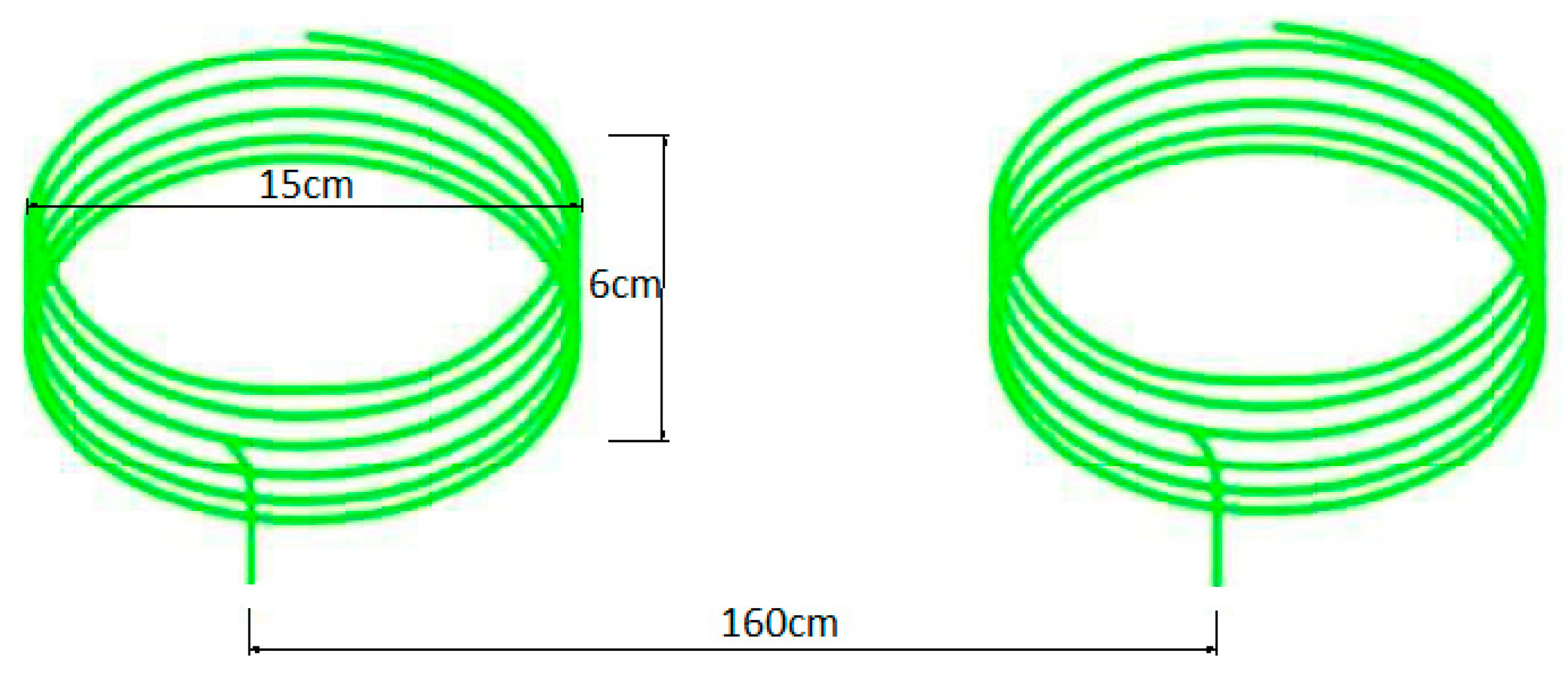
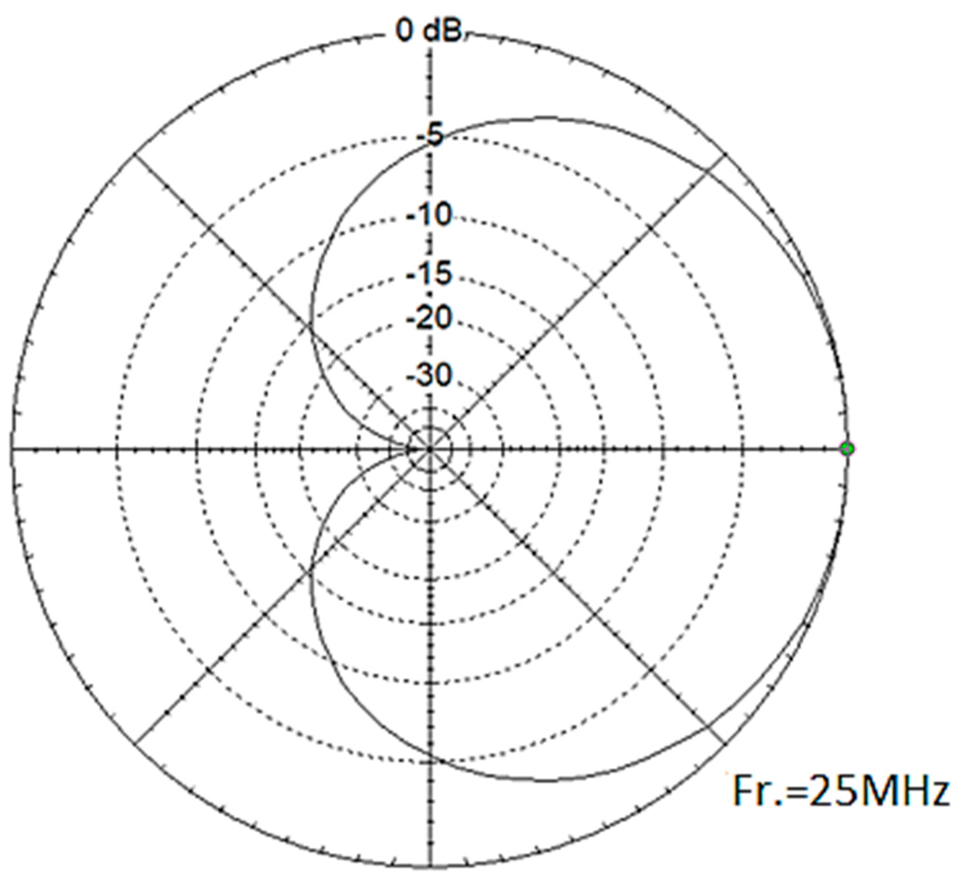
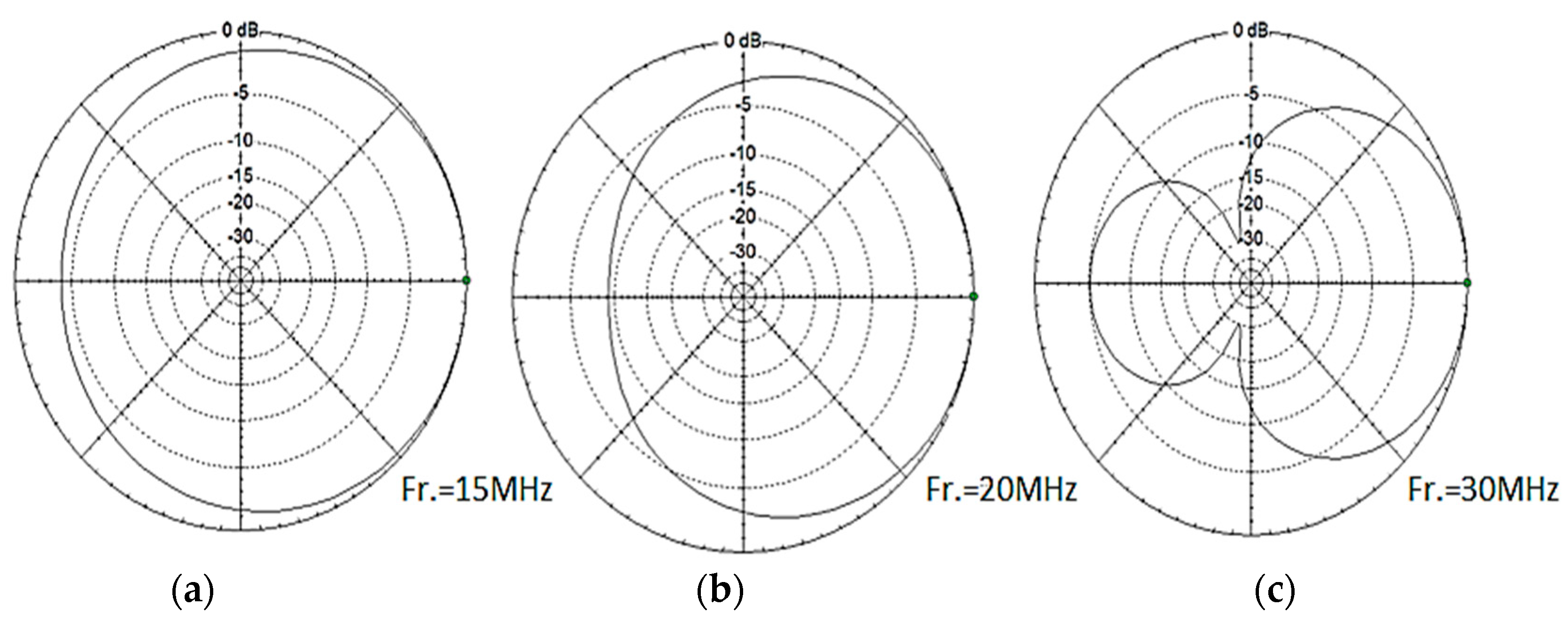
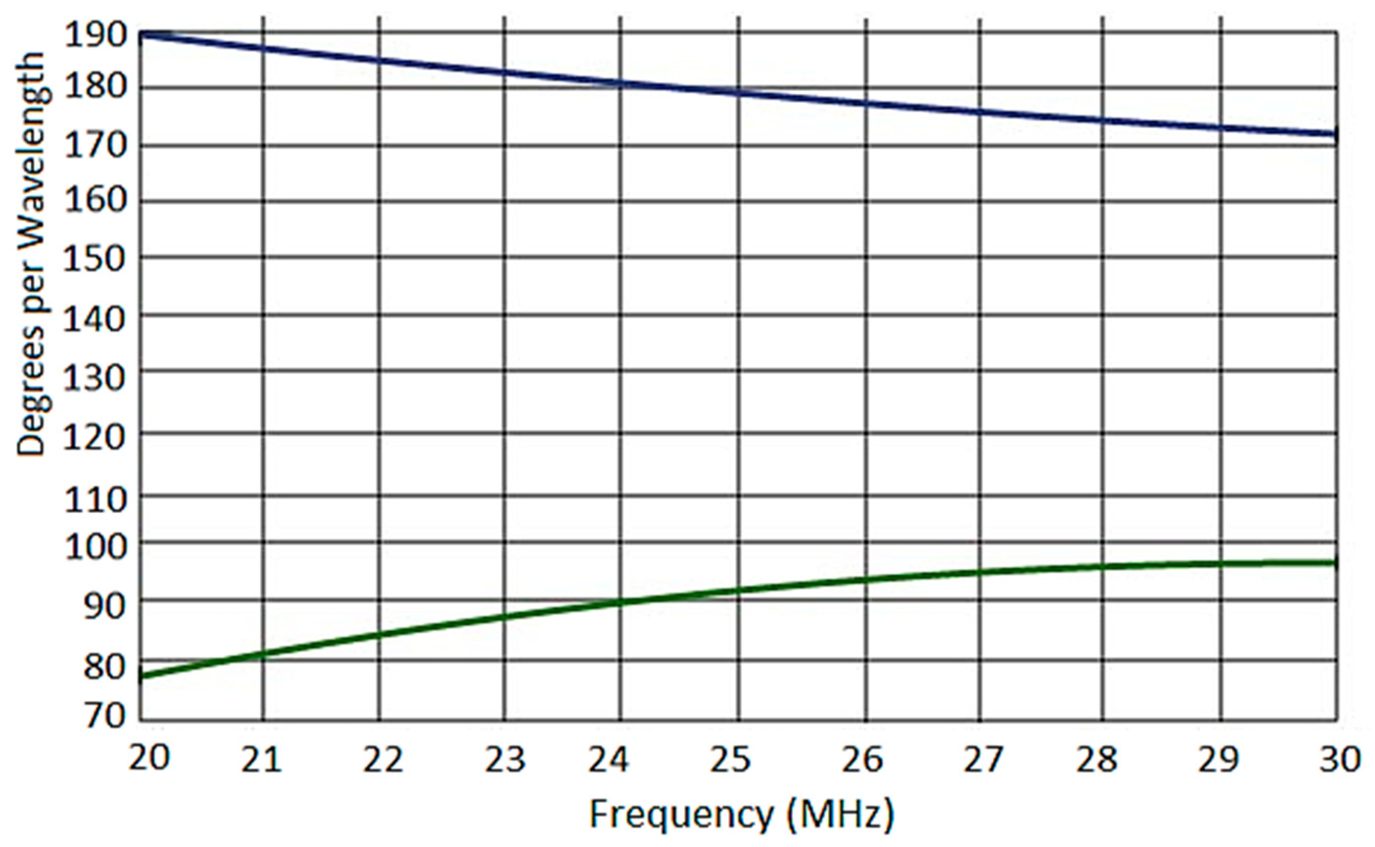
2. The Normal-Mode Helical Antenna Design Considerations

A normal-mode helical antenna (NMHA) was selected due to the fact that it functions as a circularly polarized omnidirectional antenna at a minimum size compared to any alternative at HF [10]. The helical antenna polarization sense is based on its dimensions according to Equation (1) below [11]:
C λ = S λ
where
  • Cλ: the circumference of the helix in terms of wavelengths.
  • Sλ: the spacing between turns in terms of wavelengths.
In particular, the axial ratio (AR) of the helical antenna depends solely on the dimensions of its circumference and on the distance between the turns of the coil, i.e., the pitch angle as given by Kraus in Equation (2) below:
E θ E ϕ = S λ 2 π A = 2 S λ π 2 D 2 = 2 S λ C λ 2
where
  • A: circle area;
  • D: circle diameter;
  • S: spacing between the turns of the helix;
  • λ: wavelength.
The current distribution of the normal-mode helical antenna along the helix generates two orthogonal components of the electric field: one parallel and another perpendicular to the axis of the helix. This is demonstrated by Equation (2), which expresses the far-field components EΦ and Eθ of the helix, which are in phase quadrature. Therefore, the three special cases pertaining to the NMHA polarization sense are given as follows [11]:
  • EΦ = 0 → linear vertical polarization.
  • ΕΘ = 0 → linear horizontal polarization.
  • EΦ = ΕΘ→ circular polarization.
The helical antenna operates according to the principles of a coil antenna. This implies that its design incorporates a coiled structure, which affects its impedance [12,13]. The coil structure introduces reactance into the antenna system, resulting in a reactive radiator behavior. In this respect, the NMHA typically exhibits a narrow bandwidth due to its reactive nature. To extend the narrow bandwidth of the helical antenna further, additional enhancements may be required. Various techniques and design optimizations can be employed for this purpose, as discussed in Section 2.1.
Furthermore, the gain of the helical antenna compared to that of a half-wave dipole (commonly used as a reference) remains unknown. To address these considerations, the dimensions of the two helical antennas of the array were calculated using Equations (1) and (2).
Employing Wheeler’s equation, the circumference of the helical antennas required to achieve a circular polarization radiation pattern was calculated as 15 cm. Both helices consist of 5.5 turns made of a 2.5 mm diameter copper wire, standing at a total height of 6 cm (0.05 λ) at 25 MHz. Figure 1 illustrates the helical antenna under test when operating as a standalone antenna. The circular polarization (C.P.) radiation pattern of the helical antenna operating in normal mode was simulated using EZNEC Pro2v.6.0 modeling software, as depicted in Figure 2 [14].
During the initial phase of the normal-mode helical antenna (NMHA) design, the focus was on evaluating its bandwidth as a passive radiator while considering the mismatch losses that reduce the gain of the antenna [15]. Measurements in a non-reflective environment were conducted at each desired frequency within the range 20–30 MHz using the Nano VNA-FV2 network analyzer [16]. Subsequently, the resulting impedance values were utilized in Equations (3) and (4) to calculate the reflection coefficient (Γ) and the load mismatch attenuation of the helical antennas, as illustrated in Figure 3 and Figure 4 [17].
Γ = R z 0 2 + x 2 R + z 0 2 + x 2
where
  • R: load resistance;
  • Z0: source characteristic impedance;
  • X: impedance reactive components.
Mismatch Loss = −10 Log(1 − Γ2)
According to Figure 3, the helical antenna exhibits a very narrow operational bandwidth of around 1 MHz, as expected, due to mismatch losses. In this regard, the gain of the antenna is significantly reduced to −24 dB at 30 MHz. Figure 4 presents the high-impedance plot of the helical antenna, which causes the load mismatch attenuation.
A passive helical antenna will not function effectively in a wideband mode unless coupling losses caused by the complex impedance of the helical antenna are compensated [18,19]. One approach is to employ a high-Q passive matching network to match the impedance of the helical antenna to 50 Ω when it operates off the resonant frequency [20]. However, this may not be a practical approach for a broadband antenna, which must operate efficiently across the entire frequency range. An alternative approach is to convert the passive helical antenna into an active one. This involves employing a high-input-impedance low-noise amplifier (LNA) to compensate for the coupling losses of each helical antenna across a wide frequency range. Although there is a mismatch loss at 25 MHz between the 50 Ω impedance of the helical antenna and the high input impedance of the LNA, the power gain of the entire active system, which includes the gain of the beamformer active circuit, compensates for that loss, as discussed in Section 3.1.
In the following section a detailed discussion on the high-impedance LNA design methodology is provided.

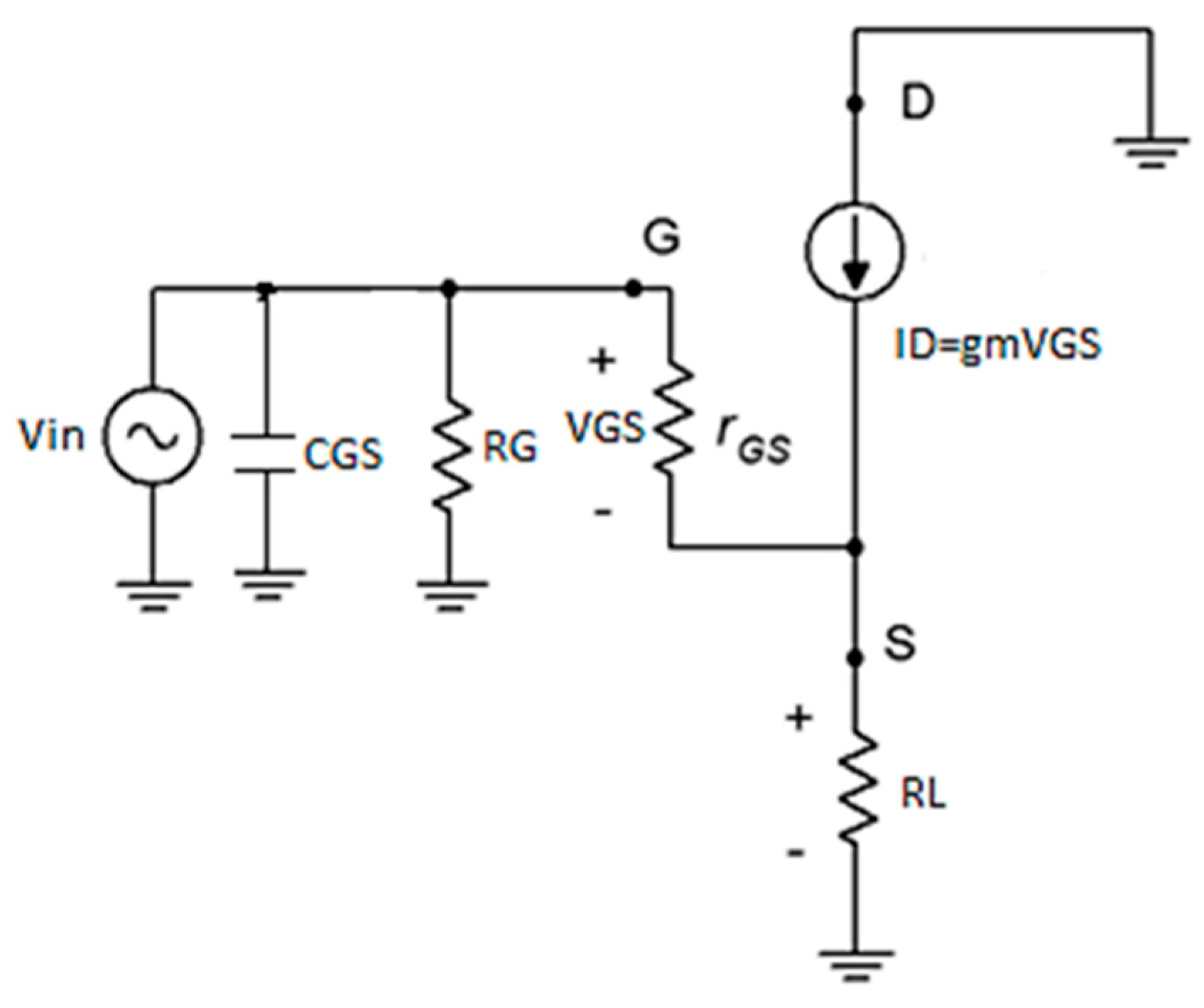
2.1. LNA Design and Implementation

The JFET (BF256B) common-drain amplifier (CDA) was utilized with a negative feedback inductor loop, serving as the initial stage of the LNA [21] and the BJT common-emitter amplifier (2N2222) as the LNA’s final stage for signal amplification [22] as illustrated in Figure 5. Internal capacitors C6, C7, and C10 are included in the schematic of Figure 5 solely for simulation purposes using Multisim 14.0 software [23]. Notably, the average gain of the cascade LNA was measured in the laboratory as −1 dB at 50 Ω, accounting for the internal capacitances of both two-stage amplifiers. This negative gain ensures stability against oscillations and minimizes the Miller effect at the input and output of the final stage [24]. A −1.5 dB attenuator at the output of the LNA isolates the Miller capacitance of the final stage to minimize the effect of the load impedance, particularly the phase specifications of the beamformer discussed in Section 3. The output attenuator is designed around a pi resistor network consisting of R10, R11, and R12, with an equivalent Thevenin resistance of 47 Ω. This confirms that the output impedance, calculated using the superposition theorem as the equivalent circuit of the resistor R7 parallel to capacitor C10, is approximately 50 Ω throughout the desired operating frequency range. The importance of the initial stage of the LNA cannot be overstated, as it has a direct impact on the signal-to-noise ratio of the received signals. For instance, due to its high input impedance, the amplifier presents a minimal load to the helical antenna, consequently preventing signal attenuation at the input of the LNA. This characteristic is crucial for minimizing losses, especially when the antenna operates away from its resonant frequency, where its impedance is significantly high, as depicted in Figure 4. In contrast, incorporating a low-impedance traditional amplifier as the first stage of the LNA results in high received signal attenuation due to the potential divider between the high impedance of the helical antenna and the low impedance of the amplifier, thereby significantly degrading the signal-to-noise ratio (SNR), regardless of the gain of the subsequent stages. Hence, the detailed analysis of the JFET CDA, following its upgrade, is further discussed below.
According to theory, the input impedance of a JFET common-collector linear amplifier is ideally very high (in the order of MΩ) [25]. However, in real-world conditions, this impedance is reduced to around 300 Ω at 25 MHz, which is relatively low due to the effect of the internal parasitic capacitances of the JFET, as shown in Figure 6. According to the superposition theorem, the gate–drain and gate–source internal capacitances of the JFET appear in parallel with the input gate resistor RG. Consequently, the input impedance of the amplifier is low at high frequencies [25]. To mitigate this, the input parasitic capacitances should be neutralized by installing a negative feedback inductor, which appears in parallel with the input of the amplifier.
To substantiate the aforementioned approach, the input impedance of the common-drain amplifier (CDA) was measured using a vector network analyzer (NANO VNA-F V2) without neutralizing the internal capacitance. The measured values are given in Table 1 below.
According to Table 1, the input impedance of the CDA is reduced due to the internal high capacitive reactance. As can be justified from the magnitude of the input impedance of the CDA, plotted in Figure 7, the input impedance of the JFET source follower amplifier is inversely proportional to frequency due to the effect of the internal capacitive reactance, already discussed.
From Table 1, we can infer that the total gate-to-source capacitance value of the BF256B, acting as a source follower amplifier, is approximately 18 pF. This value is considered in Figure 5 for simulation purposes as capacitor C6. To eliminate the capacitive reactance, a 2.2 uH negative feedback inductor (L1) was installed in parallel to the internal capacitor C6. This negative feedback inductor effectively neutralizes the parasitic capacitances at the input of the amplifier by creating a high-impedance tank circuit in parallel with the input of the amplifier. This assertion was further validated through Multisim software, as shown in Figure 8, where the input impedance of the CDA significantly increased.
According to Figure 8, the input impedance of the CDA is in the order of KΩ. Table 2 depicts the vector analyzer impedance measurements of the helical antenna. Based on these measurements, the high-impedance JFET low-noise amplifier’s performance was simulated using Multisim software.
According to the simulation results, presented in Table 2, it is evident that the aforementioned neutralization technique significantly enhanced the bandwidth of the helical antenna when applied to the high-impedance low-noise amplifier (LNA). This enables the helical antenna to function efficiently as an active antenna across a wide frequency range as discussed in the following section.

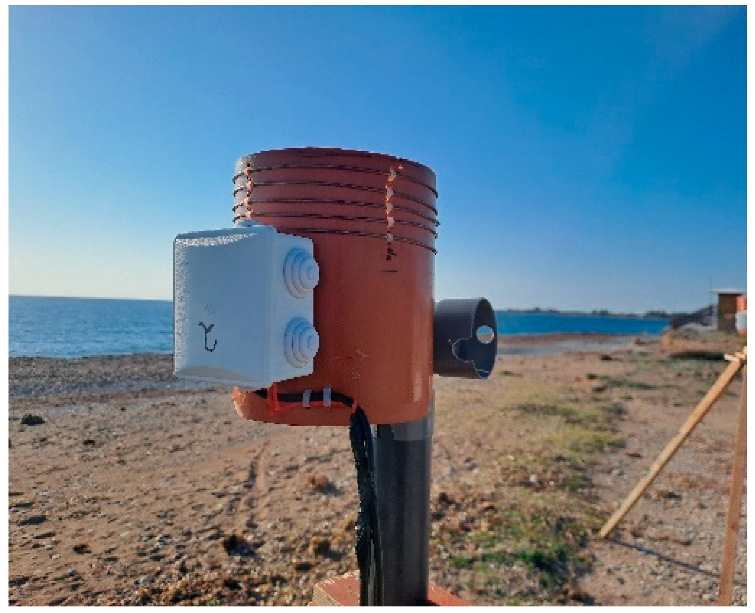
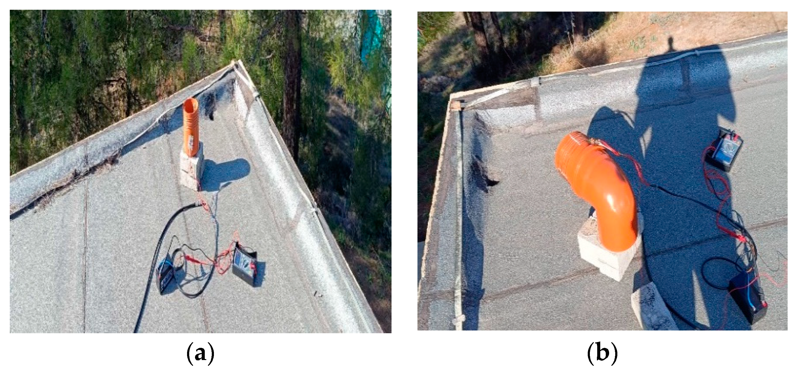
2.2. Testing the Active Helical Antenna under Real Conditions

Expanding on the simulation results detailed in Table 2, an evaluation of the helical antenna’s performance under real conditions (in a reflection-free environment) was conducted. The antenna underwent testing by receiving a transmitted signal in the 20–30 MHz range at a specific distance within the far-field zone.
Initially, the helical antenna was assessed in its passive state. Subsequent testing was conducted with the antenna in its active mode without feedback neutralization and finally as an active antenna with feedback neutralization. The test results are illustrated in Figure 9, with the blue dots representing the signal strength of the passive helical antenna directly connected to the spectrum analyzer, the orange dots signifying the active helical antenna results without feedback, and the grey dots the results after implementing inductive feedback neutralization.
As depicted in Figure 9, the resonant frequency of the helical antenna in this experiment was shifted to 27 MHz. Consequently, the high input impedance of the LNA is not particularly significant. However, by incorporating a high-impedance LNA, an enhancement in the antenna performance across the lower and upper frequency range was confirmed. This improvement is crucial because at these frequencies, the antenna impedance is very high.

2.3. Performance Improvement of the Active Helical Antenna over the Half-Wave Dipole

In this section, the performance of the active helical antenna in comparison to a passive half-wave horizontally polarized dipole is presented. The tests were conducted under real conditions in a non-reflective environment. The impedance of the monitoring reference horizontal half-wave dipole was measured at each test frequency (within 20–30 MHz) using a portable vector analyzer (NanoVNA V2). This ensured that all coupling losses of the reference dipole were accounted for in the final spectrum analyzer signal strength measurements, as depicted in Figure 10.
The active helical antenna was tested both vertically and horizontally to determine its axial ratio, a vital array design parameter. The distance between the transmitting and receiving antennas was set at 15 λ to ensure proper far-field measurements. The transmitting antenna used for the test was a half-wave horizontally polarized dipole. The signal strength values of the helical antenna under test are illustrated in Figure 10 as well. The blue curve represents the response of the reference half-wave horizontally polarized dipole. The brown and grey curves represent the respective vertical and horizontal responses of the active NMHA.
Based on Figure 10, the helical antenna exhibits an average axial ratio of 2 dB. Considering the compact size of the antenna, which is 6 cm in height operating at the 12 m band, the results are very satisfactory.

2.4. Testing the NMHA versus a Rohde & Schwarz Dual-Polarization (HE016) Active Antenna

The active helical antenna was validated against a dual-polarization active antenna (HE016), at a validation site as shown in Figure 11a, using a Rohde & Schwarz (R&S) EM510 HF digital broadband receiver (Columbia, MD, USA) shown in Figure 11b [26,27].
The helical antenna at the validation site, tested vertically and horizontally polarized, is shown in Figure 12a and Figure 12b, respectively.
Although the signals received during the test fluctuate by more than 10 dB, instantaneous measurements of the helical antenna against the active antenna (HE016) are shown in the screenshots below.
As shown from the measured spectrum of the HE016 in Figure 13a compared to that of Figure 13b, where the helical antenna was tested vertically polarized, a multitude of signals were received that could not be detected by the HE016 vertical component. This verifies that the helical antenna is capable of receiving horizontally polarized signals as well. Furthermore, despite the fluctuations in signal strength, the test results indicated that the gain of the HE016’s horizontal component in Figure 14a is similar to the gain of the helical antenna in a horizontally polarized configuration, as depicted in Figure 14b. In the following section, we discuss the helical phased array design, implementation, and evaluation in greater detail.

3. Design Principles of the Helical Phased Array

The array directivity and front-to-back ratio are defined by the amplitude and phase difference between the two helical antennas. This phase difference is determined by the spacing and orientation of the antennas, as well as by the phase shift introduced by the beamformer, which serves both as a splitter and a combiner [28]. The spacing between the helical antennas determines the necessary phase difference to steer the beam in a specific direction. The phase shift required between the two adjacent helical antennas is proportional to the wavelength and the spacing between them. Given that the two helical antennas are placed side by side λ/8 apart, which is equivalent to a distance of 1.6 m at 25 MHz, the helical array is illustrated in Figure 15.
Ψ = 2 π s λ sin θ λ Δ Φ
where:
  • Ψ: the phase of the array in a given direction;
  • Sλ: element spacing;
  • Θ: the angle of radiation;
  • ΔΦ: phase difference between the two elements;
  • λ: wavelength.
To determine the array phase difference, Equation (5) was applied [28]. The radiation pattern of the array caused by the superposition of the signals from each helical antenna is expressed by Equation (6) below [29].
A R R A Y F A C T O R = S i n ( N Ψ 2 ) 2 S i n ( Ψ 2 )
where:
  • N: the number of elements;
  • Ψ: the phase of the array in a given direction.
Using software simulation based on Equations (5) and (6) with ΔΦ = 135° and Sλ = λ/8, the radiation pattern of the two helical array is illustrated in Figure 16.
The spacing between the two helical antennas determines the array factor, which describes the combined radiation pattern of the array. The array factor can be computed using a mathematical expression that describes the complex phasor sum of the individual radiation patterns of each helical antenna in the array. It takes into account the amplitude and phase shift of each element’s contribution to the overall radiation pattern. The array gain was then computed using Equation (7) below [30].
Gain = [(cos45 + cos135)2 + (sin45 + sin135)2]0.5 = 1.41 dB or 1.5 dB
From Equation (7), it follows that the gain of the array is 1.5 dB at 25 MHz with a front-to-back ratio of 23 dB. Alternatively, by simulating the radiation pattern of the array using EZNEC, the front-to-back ratio of the resulting cardioid radiation pattern exceeds 30 dB, as illustrated in Figure 17.
Using EZNEC software, the radiation pattern of the helical array, when fed by a 135° phase shift at a distance of λ/8 at 25 MHz, was simulated at 15 MHz, 20 MHz, and 30 MHz, with the respective results shown in Figure 18a–c.
When the two-helical antennas operate off frequency, they fail to achieve proper phasing towards the desired direction, a fact supported by parameter Ψ in Equation (5), which varies proportionally to the wavelength of the spacing (Sλ) between them and inversely proportionally to ΔΦ. Consequently, this deviation causes a distortion in the radiation pattern from its ideal value, as depicted in Figure 18a, ultimately resulting in a significant reduction in the front-to-back ratio to only 4 dB at 15 MHz. This deviation can be justified by observing Figure 18b, where the radiation pattern changes from its original shape. As a consequence, the front-to-back ratio in this scenario decreases to 9 dB at 20 MHz. For the same reason, as illustrated in Figure 18c, the front-to-back ratio decreases to 5 dB at 30 MHz. To effectively address this issue, the beamformer should be engineered to feed the helices with a phase difference (ΔΦ) that varies in proportion to the spacing between them (Sλ). This adjustment ensures a consistent 180° phase shift to the backward direction of the array across the frequency range. Further elaboration on this approach is provided in Section 3.1.

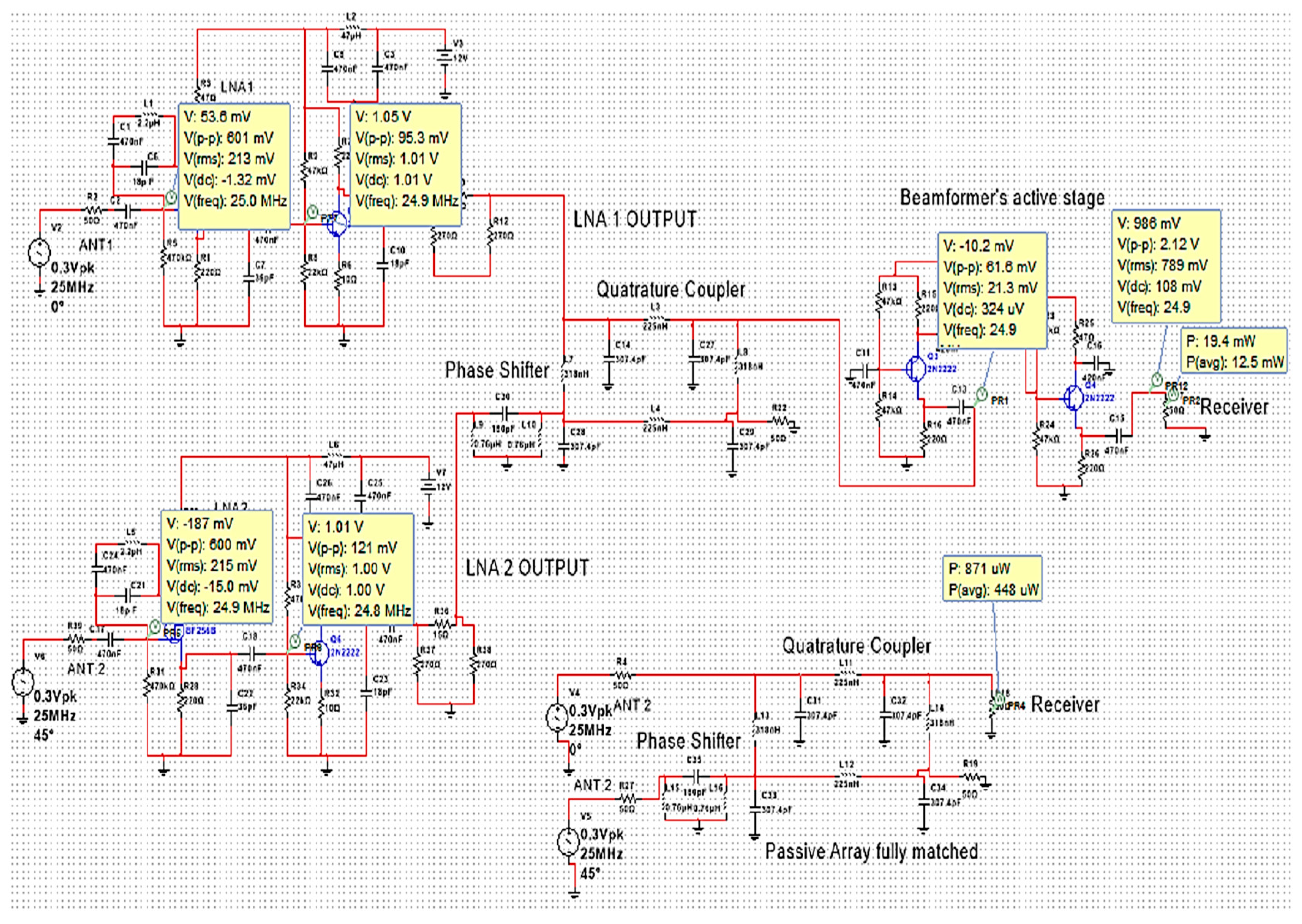
3.1. Τhe Beamformer Design and Implementation

The beamformer is crucial to the overall array performance as it controls both the phase and amplitude differences in each helical antenna relative to the phase delay of the distance between them when operating collectively as an array. The beamformer functions as a splitter and combiner circuit, consisting of a cascade phase shift network and an active circuit. The phase shift between the two helices, as illustrated earlier in Equation (5), determines ΔΦ. Furthermore, the phase delay caused by the spacing between the two helical antennas (Sλ) is a variable dependent on their distance in terms of wavelength. For instance, in scenarios where the array maintains a fixed ΔΦ value (such as with a quarter-wavelength array employing a fixed 90-degree hybrid feed), the phase difference (Ψ) outlined in Equation (5) only varies at each operating frequency due to changes in Sλ. The phase difference between the two helical antennas at each operating frequency is illustrated in Figure 19 below.
The blue curve at the top represents the phase difference between the two helical antennas when the array radiates in the backward direction. At 25 MHz, the 180° phase difference between the two helical antennas results in a theoretically infinite front-to-back ratio. As depicted in Figure 19, the highest phase error occurs at the extremes of the operating frequency range at around +5%. Conversely, the blue graph at the bottom represents the phase difference between the two helical antennas when the array radiates in the forward direction. A maximum gain of 1.89 dB occurs when the phase difference between the two helical antennas is 78.8° at 20 MHz. To minimize the phase error in the backward direction, Ψ must be constant at all operating frequencies. Therefore, a compensation circuit was implemented for this linearization. The circuit diagram of the beamformer is depicted in Figure 20. The output impedance of the two LNAs, along with the pi attenuator circuits connected to the inputs of the beamformer, is only modeled for simulation purposes.
The design philosophy of the beamformer linearization circuit is based on a consistent 180° phase difference (backward direction) between the helical antennas across all operating frequencies. This is essential for optimizing antenna performance and phase error minimization, particularly at the frequency range extremes. The aim of the compensation circuit is to maintain a stable phase relationship (Ψ) between the antennas, thus enhancing the overall array performance and ensuring reliable operation across the desired frequency range. As an example, a variable phase 45° high-pass phase shifter, integrated in series with the fixed 90° hybrid, was incorporated into one of the two inputs of the beamformer [31]. This setup aims to establish a consistent phase difference of 180° between the two helical antennas across all operating frequencies. To ensure reliability, Mini Circuits’ hybrid PSCQ-2-51W (Brooklyn, NY, USA) was utilized to introduce a fixed 90° phase shift to the network [32]. Furthermore, the common-base amplifier topology was chosen on the basis of its low input impedance, which matched the 50 Ω output impedance of the hybrid. Consequently, the common-base topology provides voltage gain, while the common collector compensates for the current gain of the two-stage amplifier [33] since its low output impedance effectively matches the 50 Ω input port (R5) of the receiver. The simulation of the entire system at 25 MHz is depicted in Figure 21 below. The system consists of the two LNAs driven by helical antennas, connected to a 45-degree high-pass phase shifter cascaded to the quadrature hybrid. Moreover, the output of the quadrature coupler is amplified by the final amplifier of the beamformer. Figure 21 illustrates the simulation of the complete system in the forward direction, compared to a fully matched passive system, respectively. As depicted in Figure 21, the active system demonstrates a power gain of 14.5 dB over the passive system.
In this regard, the assessment of the beamformer under real-world conditions is elaborated upon in Section 3.2 below.

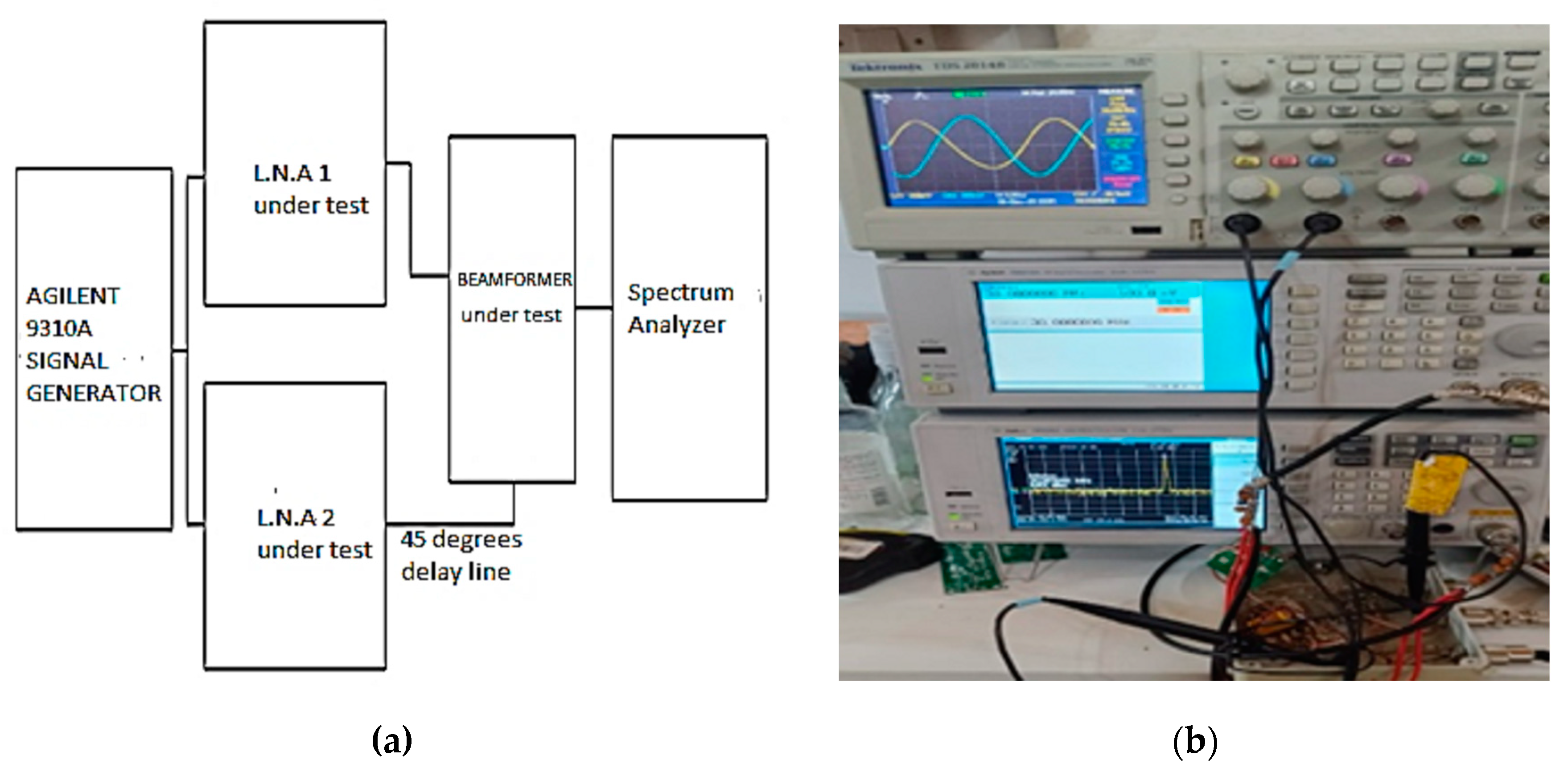
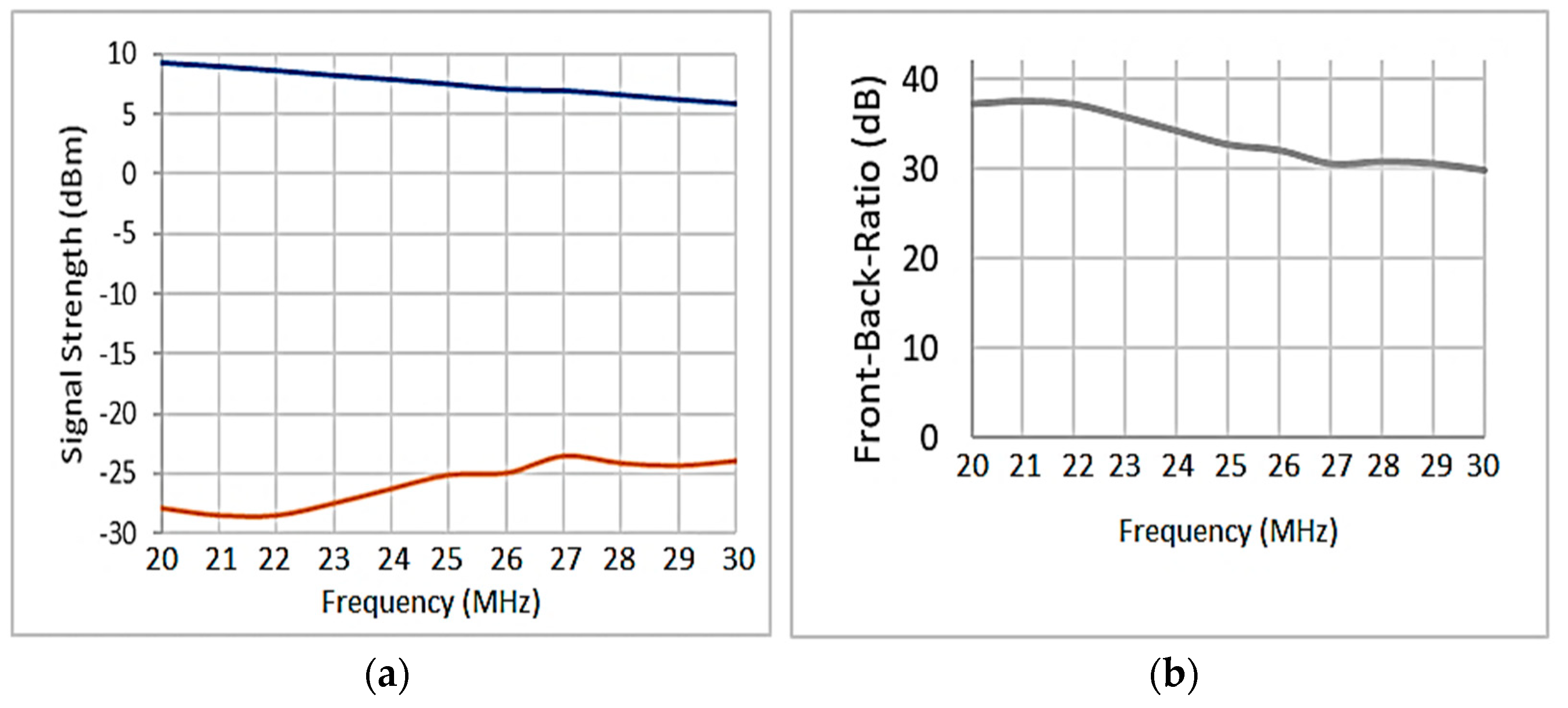
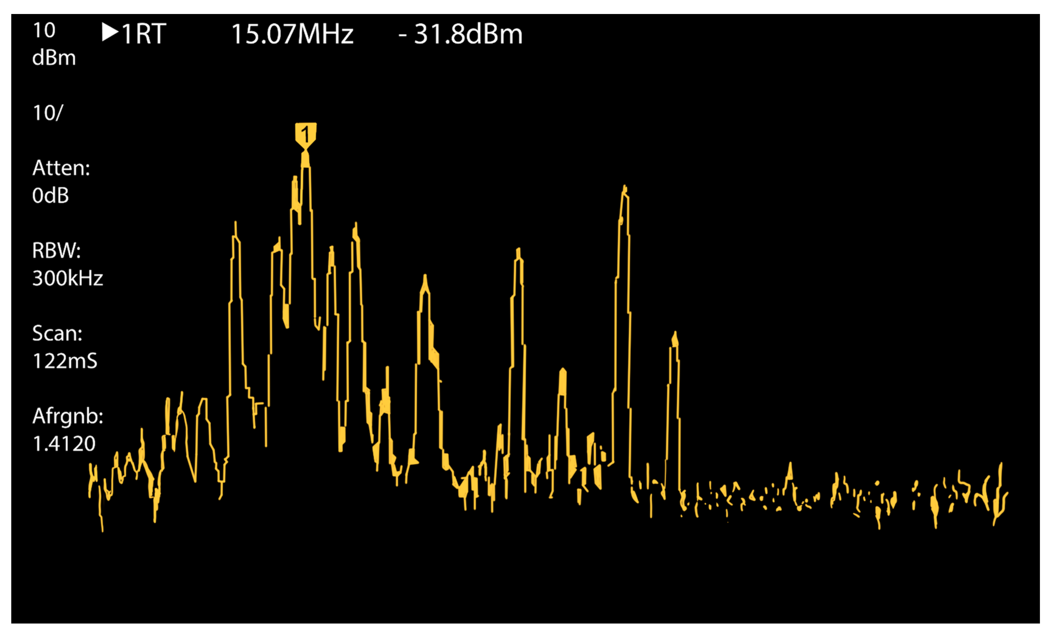
3.2. Beamformer Performance Evaluation

To evaluate the beamformer performance as a standalone unit, laboratory measurements were conducted by replacing the helical antennas with the signal generator AGILENT N9310A. Since the two helical antennas were placed side by side λ/8 apart, the phase delay between them at the input ports of the beamformer was achieved using a 50 Ω, 45° delay line. The two LNAs were integral parts of the active helical antennas and were therefore included in the test to identify any phase and amplitude imbalances between them when interacting with the beamformer, as illustrated in Figure 22a. The test setup is depicted in Figure 22b.
After numerous trials, the optimum front-to-back ratio response was achieved at 23 MHz, diverging from the original target of 25 MHz. As depicted in Figure 23 below, the phase difference between the two modeled helical antennas (blue curve at the bottom) operating within the 20–30 MHz frequency range, when ΔΦ is fixed, exhibits a positive slope in the forward direction. This problem arises due to the phase error caused by the distance between the two helical antennas as a function of the wavelength. In contrast, the phase difference in the backward direction of the array (grey graph at the bottom) exhibits roughly a linear behavior, with a phase error of approximately +2.5% due to the linearization which is attributed to the integration of a high-pass phase progressive network into the beamformer. Figure 24a shows the amplitude response of the array in both forward (depicted by the blue graph at the top) and backward (depicted by the orange graph at the bottom) directions. Furthermore, Figure 24b illustrates the beamformer front-to-back ratio under ideal conditions, ranging from a minimum value of 30 dB at 30 MHz to a maximum value of 37 dB at 20 MHz.
The average front-to-back ratio response within 20–30 MHz is at 33 dB. Despite minor amplitude imbalances between the two LNAs regarding the input ports of the beamformer, the front-to-back ratio achieved under ideal laboratory conditions is considered very satisfactory [34]. The following sections focus on the performance evaluation of the helical phased array tested under real conditions.

3.3. Final Assessment of the Helical Phased Array

To validate the performance of the helical phased array, tests were conducted under real conditions. A vertically polarized monopole served as the transmitting antenna, installed at a distance of 15 λ from the helical array. The transmission signal, generated by an AGILENT N9310A frequency generator and amplified by a 2 W HF amplifier, was utilized for the tests. Meanwhile, the helical array underwent testing in both vertical and horizontal polarizations (as shown in Figure 25). Signal strength measurements of on-air HF signals were recorded before the test using a spectrum analyzer (Tiny SA Ultra), as shown in Figure 26. Based on multiple tests, the optimum performance of the array was achieved with the two helical antennas placed 1.87 m apart. Although the helical phased array was originally designed to operate in the 20–30 MHz range, final performance tests were conducted from 15 MHz to assess its operational bandwidth at lower frequencies, where antenna dimensions play a critical role.
Figure 27a illustrates array measurements in a vertically polarized configuration. The blue plot at the top represents forward radiation, while the orange graph at the bottom shows backward radiation. Figure 27b indicates array tests in a horizontally polarized configuration. As depicted in the figures, the axial ratio of the array deviates from unity only below 15 MHz.
The measured values of the amplitude difference between the two polarizations to determine the axial ratio of the array are depicted in Figure 28a. The axial ratio exhibits a maximum deviation from unity of around 6 dB at 26 MHz within the mid-range frequencies. Additionally, at 16 MHz, 18 MHz, and 20 MHz, the axial ratio ideally approaches 0 dB. The poorest performance was observed at 15 MHz, where the axial ratio reached 30 dB, indicating that the helical array behaved as a linearly polarized antenna as was expected.
The front-to-back ratio of the helical array in vertical and horizontal polarization between 15 and 30 MHz was determined from measurements in Figure 28b. The blue and orange plots correspond to vertical and horizontal polarizations, respectively. As observed in Figure 28b, the two plots are in good agreement. For vertical polarization, the front-to-back response was 33 dB at 21 MHz and 22 MHz, respectively. At 20 MHz, the front-to-back ratio was 13 dB for vertical and 8 dB for horizontal polarization.
It is important to underline that all final tests of the array were conducted outdoors in a reflection-free environment. However, some of the measurements were affected by incoming on air signals. Nevertheless, the front-to-back ratio response of the helical array is very satisfactory, particularly when considering its extremely compact size.

4. Concluding Remarks

The study aimed to design, develop, and evaluate a compact wideband circularly polarized phased array antenna capable of delivering optimal performance across the HF spectrum, where antenna dimensions impose limitations. The proposed antenna is intended for future use in a campaign to enhance existing HF spectral occupancy models with azimuthal measurements [35]. Significant emphasis was placed on two key design components: enhancing the low-noise amplifier (LNA) and linearizing the beamformer, both crucial for optimizing the performance of the wideband circularly polarized phased array antenna. Firstly, LNA neutralization played a pivotal role in mitigating the effects of internal parasitic capacitances within the cascade LNA. By incorporating negative feedback inductors, these parasitic capacitances have been eliminated, thereby enhancing the input impedance of the LNA. This improvement in the input impedance of the LNAs minimized signal losses and maximized the signal-to-noise ratio, which is particularly critical when the helical antennas are operating away from their resonant frequency. Such meticulous neutralization ensures that the helical antennas operate efficiently across the desired frequency range (15–30MHz). The beamformer was essential for optimizing the operation of the phased array antenna. In order to maintain consistent phase difference across all operating frequencies, a compensation circuit was implemented for linearization. This circuit, comprising a variable phase 45° high-pass phase shifter and a fixed 90° hybrid, ensures stable phase relationships between the helical antennas. Additionally, the choice of a high-gain common-base amplifier topology at the output of the beamformer contributes to impedance matching between the array and the receiver and compensates for any losses caused by the mismatch of the helical antennas with the LNAs when the array operates at resonance. Furthermore, the front-to-back ratio, a crucial indicator of antenna directional performance, was found to be very satisfactory. Across both vertical and horizontal polarizations and within the frequency range of 15–30 MHz, the helical phased array antenna achieved an average front-to-back ratio exceeding 21 dB. Moreover, the axial ratio, which quantifies the polarization purity of the antenna, was measured at an impressive average of 2 dB. This indicates minimal deviation from ideal circular polarization, ensuring consistent and reliable signal reception across a wide range of azimuths. Such a low axial ratio is particularly crucial because it eliminates the need for the installation of a large and heavy circular polarization directional antenna to improve the signal-to-noise ratio (SNR) Finally, the antenna can be easily adapted to a square or circular array configuration, offering increased gain and a superior front-to-back ratio within highly constrained spaces where installing a large and heavy directional antenna would be impractical. Future research may focus on further optimization for specific operational scenarios within the 30 and 60 m bands.

Author Contributions

Conceptualization, A.C.; methodology, A.C.; formal analysis, C.K. and A.C.; investigation, A.C. and C.K.; data curation, C.K. and A.C.; writing—original draft preparation, A.C.; writing—review and editing, H.H. and S.N.; visualization, S.N.; supervision, H.H.; project administration, A.C.; funding acquisition, A.C., C.K. and S.N. All authors have read and agreed to the published version of the manuscript.

Funding

This research received no external funding.

Institutional Review Board Statement

Not applicable.

Informed Consent Statement

Not applicable.

Data Availability Statement

The original contributions presented in the study are included in the article, further inquiries can be directed to the corresponding author/s.

Conflicts of Interest

The authors declare no conflicts of interest.

References

  1. Constantinides, A.; Haralambous, H. A compact wideband active two-dipole HF phased array. Appl. Sci. 2021, 11, 8952. [Google Scholar] [CrossRef]
  2. Constantinides, A.; Haralambous, H.; Papadopoulos, H.; Makrominas, M. Models of HF interference over Cyprus. Appl. Sci. 2022, 12, 11808. [Google Scholar] [CrossRef]
  3. Haralambous, H.; Constantinides, A.; Paul, K.S. HF noise characteristics over Cyprus. Remote Sens. 2022, 14, 6040. [Google Scholar] [CrossRef]
  4. Taguch, M.; Era, K.; Tanak, K. Two Element Phased Array Dipole Antenna; ACES: Tokyo, Japan, 2007; Volume 22. [Google Scholar]
  5. Phasing Short HF Vertical Antennas—The Clark County Amateur Radio Association, Springfield, OH. Available online: https://www.w8og.org/short_antenna.html (accessed on 3 April 2024).
  6. Straw, R.D. The ARRL Antenna Book. 19th ed. ARRL: Newington, CT, USA, 2000. [Google Scholar]
  7. Fenn, A. Monopole Phased Array Antenna Design, Analysis, and Measurements, YouTube. Available online: https://www.youtube.com/watch?v=4P2mYGAbsJ0 (accessed on 6 April 2024).
  8. Kraus, J.; Marhefka, R.; Khan, A. Antennas and Wave Propagation; McGraw-Hill: New Delhi, India, 2002. [Google Scholar]
  9. Lindenmeier, H.; Reiter, L.; Ramadan, A.; Hopf, J.; Lindenmeier, S. A new design principle of active receiving antennas applied with a high impedance amplifier-diversity-module in a compact multi-band-antenna-system on a plastic trunk lid. SAE Tech. Pap. Ser. 2006. [Google Scholar] [CrossRef]
  10. Zainud-Deen, S.H.; Sharshar, H.A.; Awadalla, K.H. Synthesis of circular polarized normal mode helical antenna. In Proceedings of the IEEE Antennas and Propagation Society International Symposium 1997. Digest, Montreal, QC, Canada, 13–18 July 1997. [Google Scholar] [CrossRef]
  11. Helical Antenna—Abhinav. (n.d.). Available online: https://astro.abhinav.ac.in/Literature/Antennae/Kraus_Helix_Idea.pdf (accessed on 6 April 2024).
  12. Balanis, C.A. Antenna Theory: Analysis and Design; John Wiley & Sons: Hoboken, NJ, USA, 2016. [Google Scholar]
  13. Shin, D.-R.; Lee, G.; Park, W.S. Simplified vector potential and circuit equivalent model for a normal-mode helical antenna. IEEE Antennas Wirel. Propag. Lett. 2013, 12, 1037–1040. [Google Scholar] [CrossRef]
  14. EZNEC Antenna Software by W7EL. Available online: https://www.eznec.com/ (accessed on 6 April 2024).
  15. Zainudin, N.; Latef, T.A.; Aridas, N.K.; Yamada, Y.; Kamardin, K.; Rahman, N.H.A. Increase of input resistance of a normal-mode helical antenna (NMHA) in Human body application. Sensors 2020, 20, 958. [Google Scholar] [CrossRef] [PubMed]
  16. Nanovna. NanoRFE. Available online: https://nanorfe.com/nanovna-v2.html (accessed on 5 October 2023).
  17. Brown, M. Reflection Coefficient Calculator. 3ROAM. Available online: https://3roam.com/reflection-coefficient-calculator/ (accessed on 7 February 2023).
  18. Kilambi, S.L.; Da Cunha, M.P. Design and measurements of a small normal mode helical antenna with integrated microstrip structure. In Proceedings of the 2022 Antenna Measurement Techniques Association Symposium (AMTA), Denver, CO, USA, 9–14 October 2022. [Google Scholar] [CrossRef]
  19. Yamada, Y.; Hong, W.G.; Jung, W.H.; Michishita, N. High gain design of a very small normal mode helical antenna for RFID tags. In Proceedings of the TENCON 2007—2007 IEEE Region 10 Conference, Taipei, Taiwan, 30 October–2 November 2007. [Google Scholar] [CrossRef]
  20. Frenzel, L. Back to Basics: Impedance Matching (Part 3), Electronic Design. 2024. Available online: https://www.electronicdesign.com/technologies/communications/article/21801154/back-to-basics-impedance-matching-part-3 (accessed on 6 April 2024).
  21. BF256B.rev2—n-Channel JFET RF Amplifier—Onsemi. (n.d.-a). Available online: https://www.onsemi.com/pdf/datasheet/bf256b-d.pdf (accessed on 6 April 2024).
  22. P2N2222A Amplifier Transistors—onsemi. (n.d.-c). Available online: https://www.onsemi.com/pdf/datasheet/p2n2222a-d.pdf (accessed on 6 April 2024).
  23. Multisim Live Online Circuit Simulator (No Date) NI Multisim Live. Available online: https://www.multisim.com/ (accessed on 6 April 2024).
  24. RF Amplifier Stability Factors and Stabilization Techniques—Technical Articles All about Circuits. Available online: https://www.allaboutcircuits.com/technical-articles/rf-amplifier-stability-tests-and-stabilization-techniques/ (accessed on 6 April 2024).
  25. Engdahl, S. Electronic Devices; Greenhaven Press: Detroit, MI, USA, 2012. [Google Scholar]
  26. Rohde & Schwarz GmbH & Co KG. (n.d.). R&S®HE016 Active Antenna System. Rohde & Schwarz. Available online: https://www.rohde-schwarz.com/us/products/aerospace-defense-security/omnidirectional-mobile-and-semi-mobile/rs-he016-active-antenna-system_63493-9365.html (accessed on 7 April 2024).
  27. EM510 HF Digital Wideband Receiver—AB4OJ. (n.d.-a). Available online: https://www.ab4oj.com/dl/rs/EM510_dat_en.pdf (accessed on 7 April 2024).
  28. Mailloux, R.J. Phased Array Antenna Handbook; Artech House: Norwood, MA, USA, 2018. [Google Scholar]
  29. Hansen, R.C. Phased Array Antennas, 2nd ed.; Wiley: Hoboken, NJ, USA, 2009; pp. 1–547. [Google Scholar] [CrossRef]
  30. Addition of Vectors by Means of Components—Physics. YouTube. 2021. Available online: https://www.youtube.com/watch?v=xS-gdFgZel0 (accessed on 6 April 2024).
  31. High-Pass Low-Pass Phase Shifters. Available online: https://www.microwaves101.com/encyclopedias/high-pass-low-pass-phase-shifters (accessed on 5 April 2024).
  32. Plug-in Power Splitter/Combiner PSCQ-2-51W+-Mini-Circuits. (n.d.-e). Available online: https://www.minicircuits.com/pdfs/PSCQ-2-51W+.pdf (accessed on 7 April 2024).
  33. The Cascode Amplifier: Bipolar Junction Transistors: Electronics Textbook (No Date) All about Circuits. Available online: https://www.allaboutcircuits.com/textbook/semiconductors/chpt-4/cascode-amplifier/ (accessed on 16 April 2024).
  34. Rohde & Schwarz GmbH & Co KG (No Date) Monitoring Antennas, Monitoring Antennas|Rohde & Schwarz. Available online: https://www.rohde-schwarz.com/products/aerospace-defense-security/monitoring-antennas_229505.html (accessed on 16 April 2024).
  35. Mostafa, G.; Tsolaki, E.; Haralambous, H. HF Spectral Occupancy Time Series Models over the Eastern Mediterranean Region. IEEE Trans. Electromagn. Compat. 2016, 59, 240–248. [Google Scholar] [CrossRef]
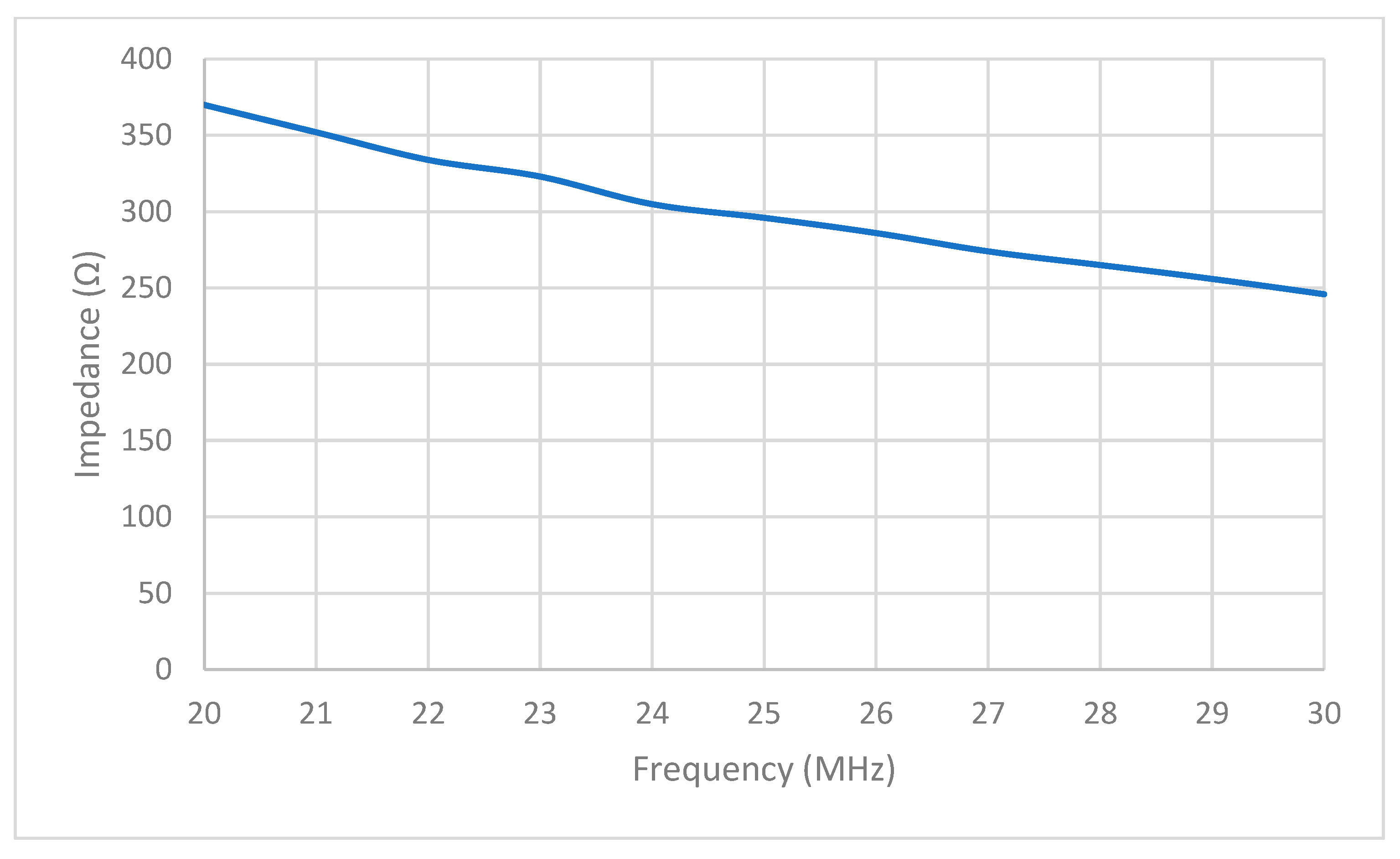
Figure 1. The normal-mode helical antenna under test.
Applsci 14 05075 g001
Figure 2. The C.P. radiation pattern of the helical antenna.
Applsci 14 05075 g002
Figure 3. The load mismatch attenuation of the helical antenna.
Applsci 14 05075 g003
Figure 4. The measured impedance of the helical across the frequency range 20–30 MHz.
Applsci 14 05075 g004
Figure 5. High-impedance two-stage low-noise amplifier circuit.
Applsci 14 05075 g005
Figure 6. The equivalent circuit of the common-drain amplifier.
Applsci 14 05075 g006
Figure 7. The input impedance of the common-drain amplifier before impedance enhancement.
Applsci 14 05075 g007
Figure 8. The input impedance of the common-drain amplifier after neutralizing input parasitic capacitances.
Applsci 14 05075 g008
Figure 9. The spectrum analyzer results of the helical antenna under real conditions.
Applsci 14 05075 g009
Figure 10. Spectrum analyzer results of the helical antenna versus the half-wave dipole.
Applsci 14 05075 g010
Figure 11. (a) The HE016 antenna under test and (b) EM510 HF digital receiver.
Applsci 14 05075 g011
Figure 12. (a) Vertically polarized helical. (b) Horizontally polarized helical under test.
Applsci 14 05075 g012
Figure 13. Spectrum of (a) HE016 vertical component, (b) helical vertically polarized.
Applsci 14 05075 g013
Figure 14. Spectrum of (a) HE016 horizontal component, (b) helical horizontally polarized.
Applsci 14 05075 g014
Figure 15. The helical array.
Applsci 14 05075 g015
Figure 16. Radiation pattern of two helical antennas placed at λ/8 apart and at 135° phase difference.
Applsci 14 05075 g016
Figure 17. The helical array radiation pattern at 25 MHz using EZNEC modeling software.
Applsci 14 05075 g017
Figure 18. EZNEC software simulation (a) at 15 MHz; (b) at 20 MHz; (c) at 30 MHz.
Applsci 14 05075 g018
Figure 19. The phase relationship between the two helical antennas.
Applsci 14 05075 g019
Figure 20. The beamformer circuit diagram.
Applsci 14 05075 g020
Figure 21. The simulation of the entire system at 25 MHz.
Applsci 14 05075 g021
Figure 22. (a) Testing arrangement. (b) Instrumentation during testing.
Applsci 14 05075 g022
Figure 23. The phase difference in the two helical antennas under ideal conditions.
Applsci 14 05075 g023
Figure 24. (a) The amplitude of the array in forward and backward directions. (b) The front-back-ratio of the helical array.
Applsci 14 05075 g024
Figure 25. Helical array tested (a) vertically and (b) horizontally.
Applsci 14 05075 g025
Figure 26. The helical array monitoring on-air HF signals using Tiny SA Ultra.
Applsci 14 05075 g026
Figure 27. (a) Array tested vertically polarized. (b) Array tested horizontally polarized.
Applsci 14 05075 g027
Figure 28. (a) The axial ratio response of the array; (b) The front-to-back ratio response of the array.
Applsci 14 05075 g028
Table 1. Common-drain amplifier input impedance values.
Frequency (MHz)Impedance (Ω)
207.3−368
216.9−j392
226.3−j337
237.0−j322
246.9−j322
256.9−j294
266.0−j285
274.8−j274
285.5−j263
295.8−j255
304.8−j245
Table 2. Multisim software simulation results based on the actual impedance of the helical antenna.
Frequency (MHz)LNA Input
(mV)
Helical Impedance
(Ω)
LNA Output
(mV)
LNA Gain
(dB)
20600457−j3517772.24
21600222−j4226851.15
2260068−j329566−0.50
2360065−j232519−1.25
2460065−j123508−1.40
2560065−j0.96544−0.85
2660062+j1456310.43
2760061+j3269524.00
2860056+j559400016.0
2960069+j900261012.0
3060048+J1450315014.0
Disclaimer/Publisher’s Note: The statements, opinions and data contained in all publications are solely those of the individual author(s) and contributor(s) and not of MDPI and/or the editor(s). MDPI and/or the editor(s) disclaim responsibility for any injury to people or property resulting from any ideas, methods, instructions or products referred to in the content.

