Abstract
Rail-fastening components are essential for ensuring the safety of urban rail systems by securing rails to sleepers. Traditional inspection methods rely heavily on manual labor and are inefficient. This paper introduces a novel approach to address these inefficiencies and the challenges faced by computer vision-based inspections, such as missed detections due to imbalanced samples and limitations in conventional image segmentation techniques. Our approach transitions the industry’s focus from qualitative to a more precise quantitative analysis of rail-fastening components. We propose Mask-FRCN, an advanced image segmentation network that incorporates three key technological enhancements: the fully refined convolutional network module (FRCN),which refines the segmentation boundaries for SFC-type fasteners; the Channel-WiseKnowledge Distillation (CWD) algorithm, which boosts the model’s inference efficiency; and the FCRM methodology, which enhances the extraction capabilities for features specific to SFC-type fasteners. Furthermore, we introduce a fastener system inspection and quantization method based on the Mask FRCN method (FIQ), a novel technique for quantifying the condition of components by using image features, template matching with random forests, and a clustering calculation method derived from segmentation results. Experimental results validate that our method significantly surpasses existing techniques in accuracy, thereby offering a more efficient solution for inspecting rail-fastening components. The enhanced Mask-FRCN achieves a segmentation accuracy of 96.01% and a reduced network size of 36.1 M. Additionally, the FIQ method improves fault detection accuracy for SFC-type fasteners to 95.13%, demonstrating the efficacy and efficiency of our innovative approach.
1. Introduction
The fastener is a component used to secure the rail to the sleeper. As a crucial part of urban rail systems, fasteners play a vital role in ensuring safe rail travel. Consequently, the safety of fasteners is closely related to the security of urban rail travel, and every fastener must be reliable. Traditionally, track fastener inspection is carried out manually, consuming significant human resources, and there is room for increased efficiency. Thus, researchers are exploring more efficient inspection methods.
Over the past decade, the rapid development of computer vision has considerably enhanced fastener inspection technology. Manual inspection has gradually evolved into a new approach, with machine inspection as the primary component and manual inspection serving as a supplementary process. Machine inspection in this context involves two steps: The first step entails capturing track images using a camera device mounted on the track inspection vehicle. The second step involves transmitting the acquired image frames to the image processing unit of the track inspection vehicle, which then determines the quality of the fasteners.
1.1. Related Works in Existing Literatures
In the early stages of computer vision development, researchers employed traditional image processing techniques for fastener detection. Xia [1] utilized the gray and gradient characteristics of the sleeper region to locate fasteners, followed by an Adaboost-based cascade classifier for detection. Feng [2] extracted Haar features for classification, creating a high-speed defect detection model. Yuan [3] introduced a direction field-based method for high-speed railways, and Liu, J. [4] developed an automatic detection system using MLPNCs. However, these methods are limited by their requirement for balanced positive and negative samples, which is a significant constraint in real-world scenarios where imbalanced datasets are common. The reliance on balanced datasets by traditional methods is a notable limitation, as it does not reflect the reality of railway maintenance where defective fasteners are relatively rare. This highlights the need for algorithms that can effectively learn from imbalanced data.
In recent years, deep learning has been applied to fastener detection. Wei et al. [5] used Faster-RCNN and YOLO V3 for railway area detection and fastener state identification. Wang [6] proposed a multi-size input training method, and Ling et al. [7] introduced a hierarchical features-based model. Liu et al. [8] and Zheng et al. [9] proposed deep learning approaches that improved performance. However, these methods still struggle with the imbalance issue and often require extensive data augmentation. Despite the advancements in deep learning, the inability of these methods to fully address the sample imbalance problem indicates a need for more innovative solutions. These approaches, although promising, still rely heavily on data augmentation, which may not always capture the nuances of real-world fastener defects.
Several studies have focused on the issue of imbalanced fastener samples. Liu et al. [10] used U-Net to obtain images containing only fasteners, then employed generative adversarial networks (GANs) to generate more fastener samples, and finally spliced the generated fastener images with blank track pictures to create new samples. Goodfellow et al. [11] introduced the concept of GANs, which have been widely used for data augmentation in various applications. Su et al. [12] employed dense fully convolutional segmentation for computerized tomography scans for contactless monitoring of railway track geometry. Muhammad et al. [13] proposed a railway fastener detection method based on the optimal selection of features and classifiers. Although these approaches address the positive and negative sample imbalance from one perspective, their essence still lies in dataset expansion to achieve a relatively balanced state of positive and negative samples. It does not genuinely eliminate the problem of sample imbalance. Furthermore, although these methods offer novel ideas for data expansion, they only demonstrate image segmentation results for fasteners under unbalanced data. The determination of fastener states obtained from image segmentation still requires human observation and a computer cannot realize one-stop detection from image input to result judgment.
1.2. Challenges to Fastener Inspection
Currently, the biggest problem in track fastener detection is still the imbalance of positive and negative samples [14], and the number of negative samples needs to be bigger so that the neural network can learn more in-depth features [15]. Additionally, most current analyses of SFC fasteners are based on qualitative analysis [16], lacking a quantitative analysis based on foreground information [17]. The qualitative nature of current analyses is a significant limitation, as it does not provide the depth of insight needed for precise fastener inspections. There is a clear gap in the literature for quantitative methods that can analyze and predict fastener conditions based on detailed foreground data.
1.2.1. Limitations of Object Detection
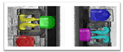
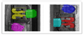
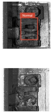
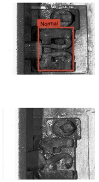
The above-discussed paper concludes that most track fastener inspection methods utilizing object-detection algorithms rely on a sufficient quantity and balance of positive and negative samples. These methods follow an “image input-output result” process, with feature acquisition and result calculation completed within the neural network, akin to a black box. However, Figure 1 shows that track fastener samples are often imbalanced [18], with a significantly smaller number of negative samples. In such cases, the performance of the object-detection algorithm is subpar [19], leading to errors in fastener detection (such as missed detections or incorrect result judgments). Consequently, object detection presents a considerable challenge in scenarios with imbalanced samples. The black-box nature of object-detection algorithms obscures the true extent of the imbalance problem. There is a need for greater transparency and interpretability in these algorithms to better understand and address their limitations in imbalanced scenarios.
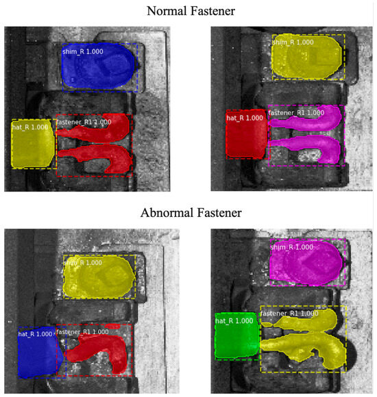
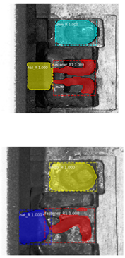
Figure 1.
When the positive and negative samples in the dataset are not balanced, the semantic segmentation algorithm is used for segmentation. The segmentation result of normal fasteners is better, whereas that of abnormal fasteners is worse.
1.2.2. The Inapplicability of Few-Shot Learning and Unsupervised Learning
Regardless of few-shot learning or unsupervised learning, the prerequisite for employing such models for training is the availability of a sufficient amount of positive and negative sample data within the same scenario. The principle of few-shot learning is that, after training a high-performing prediction model, a small number of similar objects in different scenarios is used for transfer learning to obtain a prediction model for those different scenarios [20]. However, the fastener dataset is notably small, which fundamentally undermines the feasibility of these two methods. The inapplicability of these learning paradigms underscores the unique challenges of fastener detection. The field may benefit from the development of novel learning frameworks that can adapt to the limited data scenarios common in railway maintenance.
1.2.3. Limitations of Semantic Segmentation
Semantic segmentation algorithms can achieve high-quality segmentation results for both complete and broken fasteners when provided with a sufficient dataset. However, when faced with an unbalanced dataset, the semantic segmentation algorithm can calculate complete fasteners more accurately due to their simple structure, whereas the segmentation results for damaged fasteners are poorer due to insufficient data. This results in a situation where “complete fastener segmentation is superior, whereas broken fastener segmentation yields poorer results,” as depicted in Figure 1. Nevertheless, the above two cases only complete the segmentation of fasteners, and the final state of fasteners (such as damaged or loose) still needs to be determined by examining the segmentation results. Consequently, the semantic segmentation algorithm must incorporate a final result decision step. Moreover, since the semantic segmentation algorithm predicts every pixel point, efficiency should also be considered for optimization in the practical reasoning process. The disparity in segmentation quality between complete and damaged fasteners highlights a critical need for algorithms that can accurately identify and classify fasteners regardless of their state. This requires a significant advancement in the field of semantic segmentation.
1.3. Our Contributions
This research is constrained by the challenge of sample imbalance, impacting the model’s feature learning, and lacks a quantitative analysis method for fastener conditions. Our research advances railway maintenance with innovative methodologies for SFC fastener inspection and assessment. The integration of Mask-FRCN with the FIQ method will significantly improve the accuracy and efficiency of rail fastener inspection compared to traditional methods.
(1) We have developed a novel enhancement to the Mask FRCN model, integrating the Fastener Convolutional Block Attention Module (FCRM), Fully Refined Convolutional Network (FRCN), and Channel-WiseKnowledge Distillation (CWD). This integrated approach significantly improves the segmentation and feature extraction of SFC fasteners, enabling the more accurate identification of fastener conditions. The FCRM module prioritizes key features within fastener imagery, whereas the FRCN refines segmentation boundaries for precise geometric capture. CWD distills a larger network’s knowledge into a smaller, more efficient model.
(2) We have developed an enhanced Mask FRCN model that integrates the Fastener Convolutional Block Attention Module (FCRM), the Fully Refined Convolutional Network (FRCN) module, and Channel-WiseKnowledge Distillation (CWD). This integrated approach has led to significant improvements in the segmentation and feature extraction of SFC fasteners. The FCRM module, with its attention mechanism, prioritizes the most relevant features within fastener images, whereas the FRCN module refines segmentation boundaries to capture the complex geometries with high precision. The CWD technique efficiently distills knowledge from a larger network, resulting in a compact model that maintains high performance with reduced computational resources.
(3) We introduced the FIQ method, which utilizes a template-matching approach with random forests for fastener status assessment. This method capitalizes on the enhanced segmentation from the Mask FRCN model to quantify the condition of fasteners based on image features. The FIQ method provides a systematic evaluation of fasteners, including damage and displacement, through a clustering calculation method. It has improved the fault detection accuracy of SFC-type fasteners, demonstrating the method’s efficacy and efficiency in automated fastener assessment.
2. Overview of Fastener Inspection Method
In this paper, we propose a novel detection method for track fastenings with unbalanced positive and negative samples, comprising two stages. In the first stage, we introduce a new semantic segmentation algorithm tailored for the SFC fastenings system based on Mask RCNN—Mask FRCN, which is employed to segment the fastener system and obtain the connected domain. In the second stage, we present a fastener state quantization system based on machine learning algorithms, enabling the computer to acquire the fastener state evaluation using the image-connected domain.
2.1. Semantic Segmentation Algorithm Based on Track Fasteners—Mask FRCN
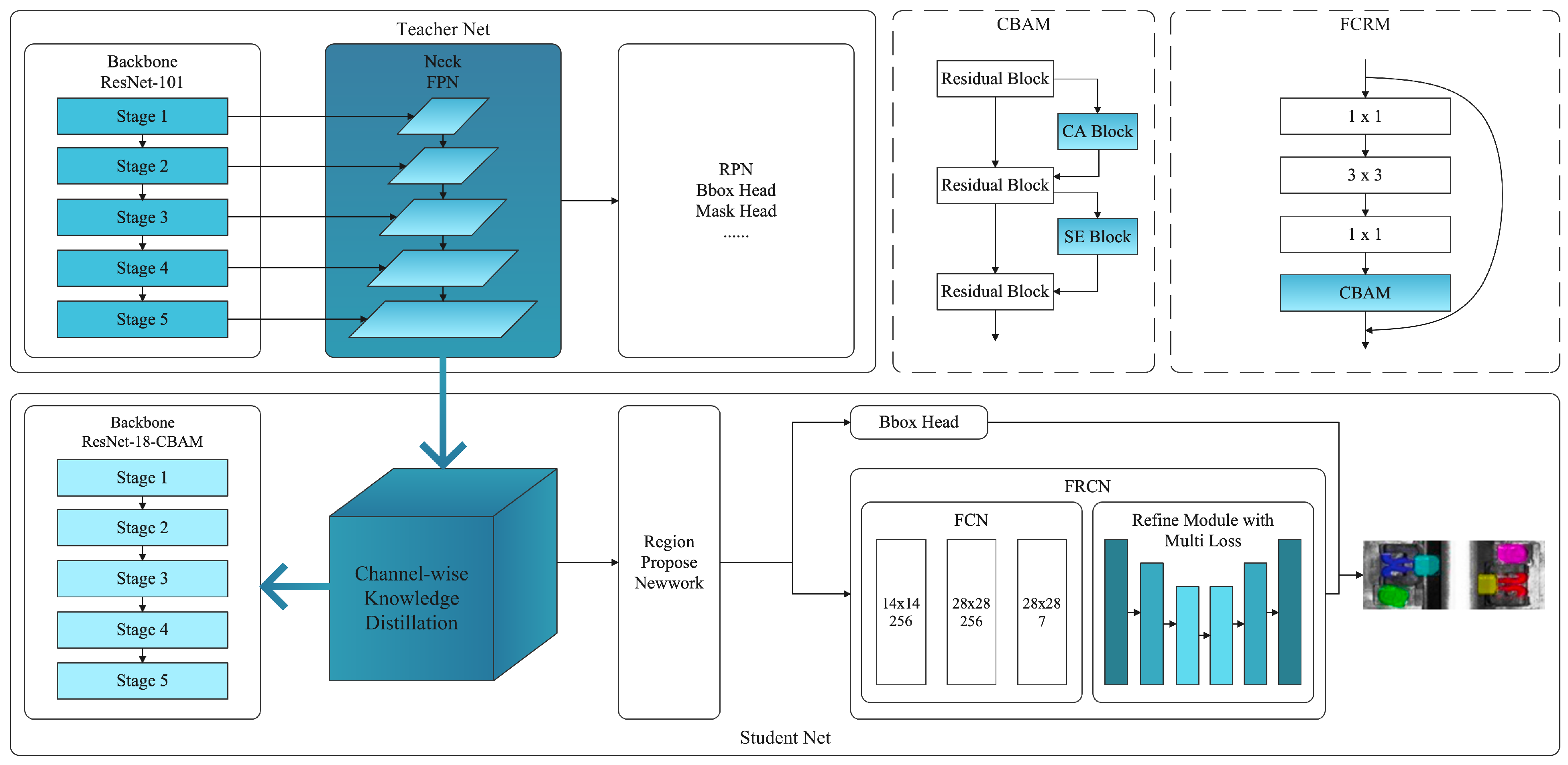
As the fastener dataset exhibits an imbalance between positive and negative samples, the final inference process may result in a scenario where “normal fasteners exhibit better reasoning outcomes, whereas abnormal fasteners demonstrate inferior reasoning performance”. To address this issue and the slow inference speed caused by the numerous parameters of the semantic segmentation algorithm, we developed a segmentation algorithm tailored to track fastener scenes, called Mask FRCN, as Figure 2 shows.

Figure 2.
The Mask FRCN framework synergizes FCRM for enhanced feature extraction, FRCN for precise edge detection, and CWD for efficient knowledge transfer between ResNet models, ensuring accurate and efficient fastener inspection.
The algorithm incorporates a refined module at its tail, allowing for more accurate segmentation of the connected domain of normal fasteners. Furthermore, to optimize the model size and inference speed, Knowledge Distillation (KD) is employed to compress the network volume. Simultaneously, a Convolutional Block Attention Module (CBAM) is integrated into the ResNet’s residual module to construct a residual attention module, thereby enhancing the boundary extraction habitability of the connected domain.
2.2. Fastener Quantization System
Upon obtaining the image-connected domain through the semantic segmentation algorithm, this paper introduces a fastener state quantization system based on the connected domain post-image segmentation. This system is founded on machine learning algorithms and encompasses system index weight construction as well as novel fastener system state evaluation.
In this system, multiple set indexes are chosen for connected domains of fasteners, fastener hats, and shims. The index weights are constructed using the random forest algorithm. The fastener system state’s quantitative calculation is achieved through feature weighting computation, ultimately completing the actual state evaluation of the fastener based on image segmentation. With this method, we can realize substantial inception as Figure 3 shows.
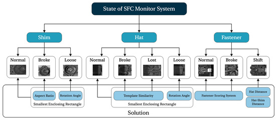
Figure 3.
This system for designing railway fasteners enables one-stop testing of fasteners, shims, and fastener hats. For fasteners, the system can evaluate damage and shift, whereas for fastener hats, it can evaluate damage, loss, and looseness. As for shims, the system can evaluate them for looseness and damage.
3. Semantic Segmentation Algorithm Based on Track Fasteners—Mask FRCN
In this section, we present Mask FRCN [21], an image segmentation algorithm specifically tailored for track fastening scenes. The architecture of this algorithm can be divided into three stages. The first stage involves feature extraction, primarily governed by the backbone. The second stage is the feature fusion stage, dominated by Feature Pyramid Networks (FPNs). The third stage comprises three prediction header networks, including two detection networks for object detection and a semantic segmentation header network for object segmentation.
Initially, ResNet-101 [22,23] was chosen as the feature extraction network, and a Residual Attention Module was constructed. To achieve improved segmentation results and ensure that more profound image features are extracted at the initial stage of network training, a CBAM attention mechanism [24] was added to the tail of the residual module at each stage. Next, to address the issue of semantic segmentation algorithms having numerous computational parameters and slow inference speeds, Channel-Wise Knowledge Distillation (CWD) [25] was employed in KD to perform knowledge distillation on the FPN backbone. CWD distilled the knowledge from ResNet-101 into ResNet-18, reducing the model size by eliminating redundant parameters while enhancing a portion of the accuracy.
Lastly, to refine the network segmentation algorithm’s head prediction network, this paper introduces an edge-refinement module based on the image-segmentation algorithm, FRCN, which aims to improve the accuracy of normal fastener segmentation.
3.1. FCRM: Fastener CBAM Residual Module
By incorporating the CBAM (Convolutional Neural Network Attention Module) into the bottleneck residual module, we constructed a bottleneck residual module with an attention mechanism called FCRM (Fastener CBAM Residual Module). In this new module, CBAM can extract spatial and channel-related information, thereby enhancing the performance of the model in the segmentation task of rail fastener-connected regions. The following is a detailed composition of the CBAM-enhanced bottleneck residual module, based on the description above:
(1) First layer: A 1 × 1 convolutional layer that reduces the number of channels. This layer typically includes batch normalization and an activation function (e.g., ReLU). The layer can be represented as follows:
(2) Second layer: A 3 × 3 convolutional layer that extracts spatial features. Similarly, this layer also includes batch normalization and an activation function. The layer can be represented as follows:
(3) Third layer: A 1 × 1 convolutional layer that restores the number of channels. This layer includes only batch normalization and typically does not include an activation function. The layer can be represented as follows:
(4) CBAM is introduced after the third convolutional layer and comprises channel attention and spatial attention [26]. Channel attention processes the input feature map with global average pooling and global max pooling, generating attention vectors that are normalized to obtain channel attention weights. These weights are applied to the third convolutional layer’s output. Spatial attention uses a convolution operation on the feature map, normalizing the output with a Sigmoid activation function to obtain spatial attention weights, which are then applied to the feature map.
(5) Skip Connection adds the input feature to CBAM’s output, forming a residual connection with the attention mechanism. This structure helps avoid gradient vanishing and representational bottleneck issues, allowing for deeper network structures.
(6) The activation function (e.g., ReLU) processes the output of the skip connection to obtain the final output of the CBAM-enhanced bottleneck residual module.
Integrating this module into ResNet-101 creates a more powerful feature extractor, where spatial and channel attention mechanisms enhance the model’s performance. Channel attention identifies channels with more task-related information, whereas spatial attention focuses on important image regions.
With the improved ResNet-101 as the backbone network for Mask R-CNN, the model performs better in rail fastener-connected region segmentation tasks. The CBAM-enhanced bottleneck residual module enables focusing on key areas and identifying task-related channels, improving Mask R-CNN’s accuracy and supporting railway safety and maintenance.
3.2. Channel-Wise Distillation Based in Mask-RCNN
The distillation process employing the Channel-Wise Distillation (CWD) algorithm, which emphasizes the neck layer of Mask R-CNN integrated with the Feature Pyramid Network (FPN), consists of multiple stages. Initially, a ResNet101 model is pre-trained to serve as the teacher model, whereas a student model with a ResNet18 architecture is established. Subsequently, the neck layer, which utilizes FPN in Mask R-CNN, is designated as the target layer for distillation. FPN combines high-level and low-level features from various layers of the network, enhancing detection and segmentation capabilities.
Channel-Wise Distillation (CWD) is a channel-based distillation approach that aims to minimize the distance between the teacher and student models’ channel feature maps. The CWD loss function is expressed as follows:
where represents the Channel-Wise Distillation loss, N denotes the number of channel pairs, and and correspond to the i-th channel feature map of the teacher and student models.
Throughout the training process, channel feature maps are extracted from the FPN layers of both the teacher and student models. For each corresponding pair of teacher and student channel feature maps, the L2 distance between them is calculated. The CWD loss function is subsequently defined as the average of the L2 distances across all channel pairs. The student model is trained using backpropagation, striving to minimize the CWD loss while concurrently optimizing the primary task loss (e.g., object detection and instance segmentation loss). This procedure iterates until convergence is reached or a predefined stopping criterion is fulfilled.
By adopting the CWD knowledge distillation algorithm to replace ResNet101 with ResNet18 in Mask R-CNN, a degree of performance improvement can be achieved. The ResNet18 architecture is more lightweight than ResNet101, thereby reducing the model’s computational complexity and memory footprint, and accelerating inference speed. Although the reduction in model size may potentially impact overall accuracy, the CWD algorithm ensures that the student model retains essential knowledge from the teacher model, mitigating performance loss.
3.3. FRCN—A Method to Improve Image Segmentation Boundary
In this section, we propose the Fully Refined Convolutional Network (FRCN), a deep learning-based image segmentation module. Traditional segmentation methods tend to result in blurry and imprecise boundaries at the edges of rail fasteners, which leads to a decrease in segmentation accuracy and precision. To address this issue, the present study proposes the use of FRCN to optimize the boundaries of image segmentation. Although the data have already undergone segmentation, the boundaries of the segmentation are not precise enough, and hence, further optimization using FRCN is necessary to improve the accuracy and precision of the segmentation.
The FRCN architecture consists of six convolutional layers and six deconvolutional layers as Table 1 shows, each of which includes convolution, batch normalization (BN), and ReLU activation function. The detailed architecture is shown in the equation below, where conv denotes convolution operation, deconv denotes deconvolutional operation, BN denotes batch normalization operation, and ReLU denotes ReLU activation function. Input and output dimensions of each convolutional and deconvolutional layer are given in parentheses.

Table 1.
FRCN layers and operations.
The FRCN architecture uses various convolution kernel sizes and strides to adapt to images of different sizes. The kernel size of the first layer is 3 × 3, with a stride of 1, whereas the kernel size and stride of subsequent convolutional layers are 3 × 3 and 2, respectively. The deconvolutional layers use upsampling techniques to restore smaller image dimensions, with the kernel size and stride of the deconvolutional layer both being 3 × 3.
In addition to the convolutional and deconvolutional layers, FRCN includes multiple fully connected layers for further feature processing and optimization. FRCN uses two fully connected layers to map features to 128 dimensional and 64 dimensional spaces, respectively, to improve feature representation.
In summary, FRCN uses multiple convolutional and deconvolutional layers, fully connected layers, and a global context attention mechanism that effectively optimizes image segmentation boundaries and improves segmentation accuracy and precision.
4. FIQ—A Fastener System Inspection and Quantization Method Based on Mask FRCN
This section addresses the issues that exist in evaluating the state of track fasteners, including imbalanced positive and negative samples, small sample sizes in target detection, and the possibility of inconclusive diagnosis results from image segmentation. To address these issues, this study proposes a track fastener quantification method based on image segmentation results—FIQ.
Specifically, this study utilizes a feature extraction algorithm based on track fastener boundaries, which effectively extracts boundary features and enables the positioning and classification of the track fasteners. Additionally, a random forest algorithm is employed to assign weights to the different states of the fasteners based on their respective conditions. For the calculation of fastener hats and pads, a feature distance-based clustering algorithm is used to effectively evaluate the different states of the fasteners.
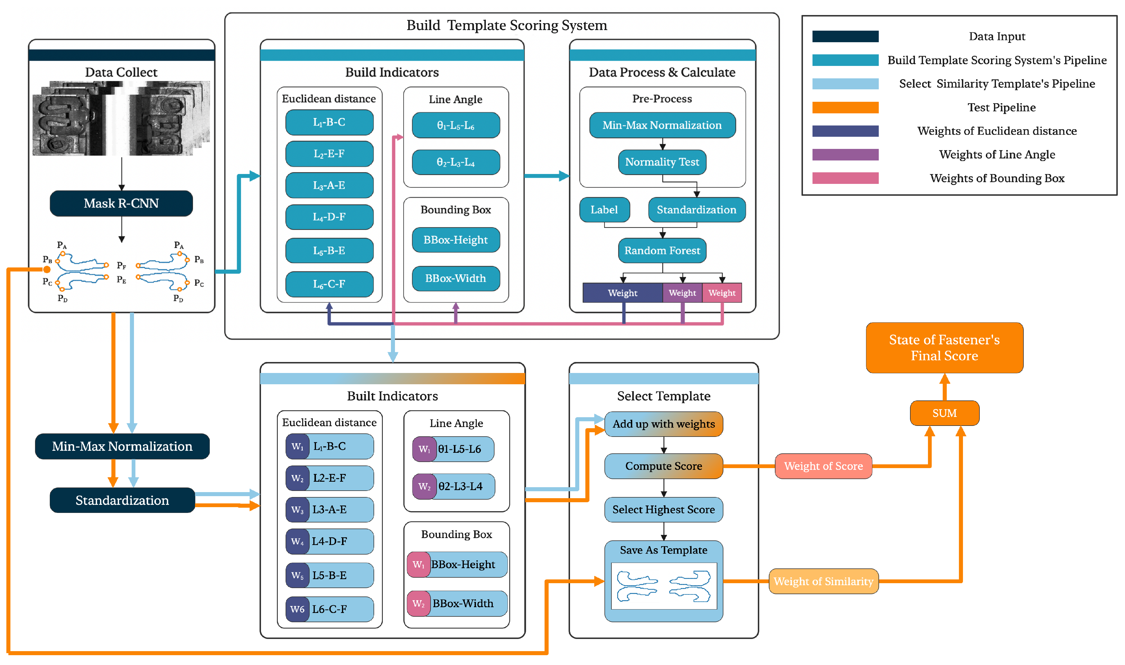
The FIQ involves two evaluation methods. For fasteners, we propose a fastener status evaluation system based on the random forest algorithm as Figure 4 shows. This algorithm selects feature points from the image segmentation results for feature calculation, such as feature distance and feature angle. It obtains a preliminary status evaluation system by calculating scores in the existing fastener dataset and selecting the fastener with the highest score as the template. The preliminary scoring system is then subjected to secondary random forest weight allocation with the fastener template to obtain the final fastener status quantification evaluation system, thereby completing the assessment of fastener broken and loss.

Figure 4.
The system employs MASK-FRCN for initial rail clip segmentation, extracting six key feature points per clip. It evaluates clip quality by calculating geometrical indicators from these points and uses a random forest to determine feature weights, resulting in a final quality assessment.
For fastener hats and shim, we propose a clustering algorithm based on image features. It clusters the feature results of the existing dataset’s segmentation results to obtain the clustering center value, thereby completing the status evaluation of fastener hats and shim. Now, we will describe in detail how to achieve a one-stop inspection of fasteners, fastener hats, and shims through a system.
4.1. For Fasteners
We used the FIQ quantification system to segment the input fasteners and obtain scores based on image features through FIQ. We also clustered the distances of the feature points of the fastener hat and calculated the distance between the clustering center points of the input fastener hats. If it is greater than the threshold, the fastener is considered to be displaced.
4.2. For Fastener Hats
We calculated the score by similarity with the template’s connected domain and then computed the clustering center value of the score with the other scores. If it is less than the damage threshold, the fastener hat is considered damaged. We also determined if the fastener hat is lost or loose by computing the minimum bounding rectangle rotation angle of the connected domain of the fastener hat.
4.3. For Shims
We calculated the score by similarity with the template’s connected domain and then computed the clustering center value of the score with the other scores. If it is less than the damage threshold, the shim is considered to be damaged. We also determined if the shim is loose by calculating the minimum bounding rectangle rotation angle of the connected domain of the shim.
4.4. A Quantization Method Based on Random Forest to Estimate Fastener Status
In this section, we proposed the Fully Refined Convolutional Network (FRCN), a deep learning-based image segmentation module. Traditional segmentation methods tend to result in blurry and imprecise boundaries at the edges of rail fasteners, which leads to a decrease in segmentation accuracy and precision. To address this issue, the present study proposes the use of FRCN to optimize the boundaries of image segmentation. Although the data have already undergone segmentation, the boundaries of the segmentation are not precise enough, and hence, further optimization using FRCN is necessary to improve the accuracy and precision of the segmentation. Here is the paragraph split into several parts:
We propose a method for evaluating the quality of fasteners based on random forest. The method includes the following steps:
1. Selecting six feature points, including the top, bottom, and leftmost and rightmost points, as well as the top vertex and bottom point of the boundary, by segmenting the boundary of the fastener.
2. Calculating the Euclidean distance between each pair of feature points and the angles between the points, which yields four lines , , , and , as well as the angles , , respectively. The Euclidean distance between two points and is calculated using the formula:
3. Using random forest to calculate the weights of the image features that determine the state of the fastener by annotating the fasteners in the existing dataset as normal, damaged, or missing. Random forest is a type of ensemble learning method based on decision trees that can improve the robustness and generalization of the model by randomly sampling and selecting features to construct multiple decision trees.
4. Assigning weights to the features to obtain a preliminary evaluation system that can preliminarily assess the quality of the fastener. The physical quantities used in this method include the Euclidean distances , , , , , , the angles and , as well as the fastener-connected component area, fastener detection box length, and fastener detection box height.
5. Combining the evaluation system with the fastener template with the highest score obtained by evaluating the existing dataset using the system and using a second random forest weight assignment to obtain the final evaluation system. This can more accurately assess the quality of the fastener and improve the objectivity and accuracy of the evaluation.
The weight of each feature contributes to the final evaluation system and can be calculated using the following formula:
where n is the number of training samples, is the predicted value of the j-th sample, is the true label of the j-th sample, is the loss function that measures the difference between and , and is the gradient of the loss function with respect to the i-th feature of the j-th sample.
The proposed method for evaluating the quality of fasteners based on random forest has several advantages. Firstly, the method selects feature points and calculates image features that can more comprehensively reflect the state of the fastener. Secondly, the random forest algorithm is used to calculate the weights of the image features, which can more accurately evaluate the quality of the fastener. Thirdly, the weights are calculated using a formula that can reduce the impact of subjective factors on the evaluation results, improving the objectivity of the evaluation. Finally, the use of a second random forest weight assignment after selecting a fastener template with the highest score can further improve the accuracy of the evaluation system. Overall, the proposed method has great potential for practical applications in evaluating the quality of fasteners. In this method, the weight of each feature contributes to the final evaluation system and can be calculated using the formula .
4.5. A Quantization Method Based on Cluster Method to Estimate Fastener Hat and Shim Status
This study proposes a clustering-based image feature calculation method to solve problems such as fastener shift, fastener hat damage/loss, and shim shift. The method can be represented by the following formula:
Here, X represents the existing dataset, and represents the feature vector of the ith image. We extract features of each component to obtain the feature vector of each image. Then, we perform clustering analysis on these feature vectors to obtain cluster centers, as follows:
Here, represents the set of cluster centers and represents the vector of the ith cluster center. We use segmentation and connected domain similarity calculation to obtain similarity clustering center values for fasteners, shims, and fastener hats. For the looseness of shims, we cluster the deflection angle of the connected domain and calculate the deviation from the center value to determine if there is looseness. For the looseness of fasteners, we determine the length of the fastener hat connecting line and its distance to the clustering center to judge the degree of looseness.
Specifically, we calculate the distance between each image’s feature vector and the cluster center to determine if it is abnormal. For fasteners and shims, we use Euclidean distance to calculate the following distance:
Here, M represents the dimension of the feature vector. For fastener hats, we use the Manhattan distance to calculate the distance, as follows:
We set a threshold to determine if it is abnormal. If the distance is less than the threshold, it is considered abnormal.
In summary, this study proposes a clustering-based image feature calculation method, which can be represented by the formula. This method can effectively detect fastener shift, fastener hat damage/loss, and shim shift, providing a reliable detection method for industrial production. Following are the fastener system inception details based on a cluster idea.
4.5.1. Fastener Shift
In this section, as Figure 5 shows, the shift calculation is performed by selecting the Euclidean distance between the left fastener cap and the left shim, the Euclidean distance between the right fastener cap and the right shim, and the Euclidean distance between the two fastener caps.
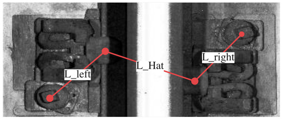
Figure 5.
The method of calculating the minimum external rectangle.
The calculation process involves clustering the existing dataset to obtain the normal and abnormal center values of these three features. The distance between the feature that needs to be judged and the normal and abnormal center values is calculated, and if the distance is closer to the normal center value, there is no problem. If it is closer to the abnormal center value, the next step of judgment is entered: by calculating the normal and abnormal center values of two fastener caps and shims corresponding to each other twice, it is determined which side of the fastener has shifted. Finally, classification is performed based on the degree of shift to determine if there is a problem.
The method is shown as Algorithm 1 and fastener shift detection definition is shown as Table 2.
| Algorithm 1 Fastener shift detection |
|
Table 2.
Fastener shift detection definition.
4.5.2. Method for Identifying Loose Fastener Hats or Shim
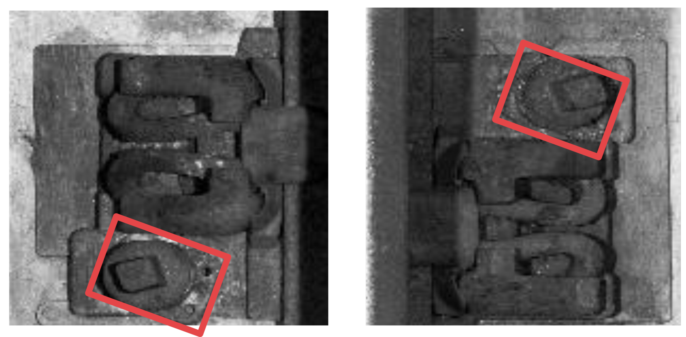
As Figure 6 shows, to do this, the minimum bounding rectangle is obtained from the connected components of the segmented image, and the rotation angle is calculated to align the part horizontally. If the angle is not equal to zero, then the part is determined to be loose.

Figure 6.
The method of calculating the minimum external rectangle. The red rectangular box represents the smallest external rectangle of the section.
4.5.3. Detecting Missing or Damaged Fasteners or Shim
To accomplish this, a template-connected component is selected from an existing dataset and compared to the connected components of the test image for similarity. The final score is computed based on this comparison. If the score is greater than 0.95, the part is classified as normal. If the score falls between 0.95 and 0.25, the part is classified as damaged, and if the score is less than 0.25, the part is classified as missing.
4.5.4. Shim Broken Inception
Each shim-connected component is selected by using the minimum bounding rectangle of the shim-connected component, and clustering is performed on the length and width of the minimum bounding rectangle of each shim-connected component in the existing dataset to obtain the center values of normal and abnormal. The difference between the normal and abnormal center values is calculated for the feature distance that needs to be evaluated. If the distance is closer to the normal center value, then there is no problem. If the distance is closer to the abnormal center value, then the shim is considered damaged. The algorithm is shown as Algorithm 2, and the variable definition is shown as Table 3.
| Algorithm 2 Shim evaluation algorithm |
|
Table 3.
Variables used in the shim evaluation algorithm.
5. Experiment Results
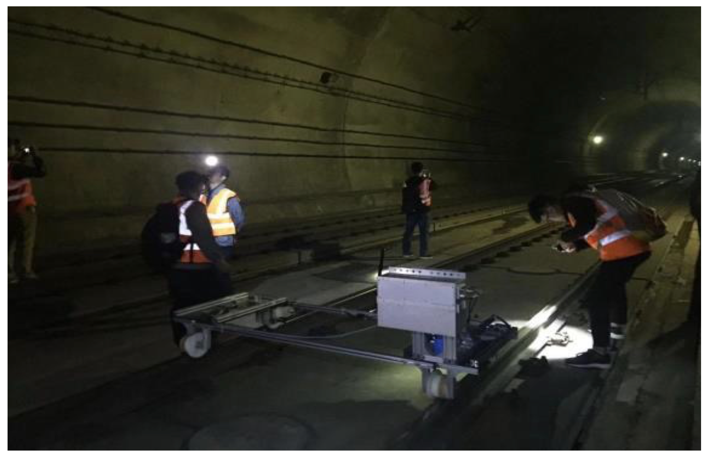
As Figure 7 shows, the industrial-grade line scan camera model LQ-C4-208D1 is selected as the imaging device for capturing track line images, parameters can be shown as Table 4, enabling long-distance image acquisition. The camera is mounted on the rail-inspection equipment and is controlled using synchronized encoder pulses. This setup facilitates the image acquisition of SFC-type fasteners discussed in this paper, as Figure 8 shows.

Figure 7.
LQ-C4-208D1 railway detect car.
Table 4.
Parameters of the LQ-C4-208D1 line scan integrated imaging module.

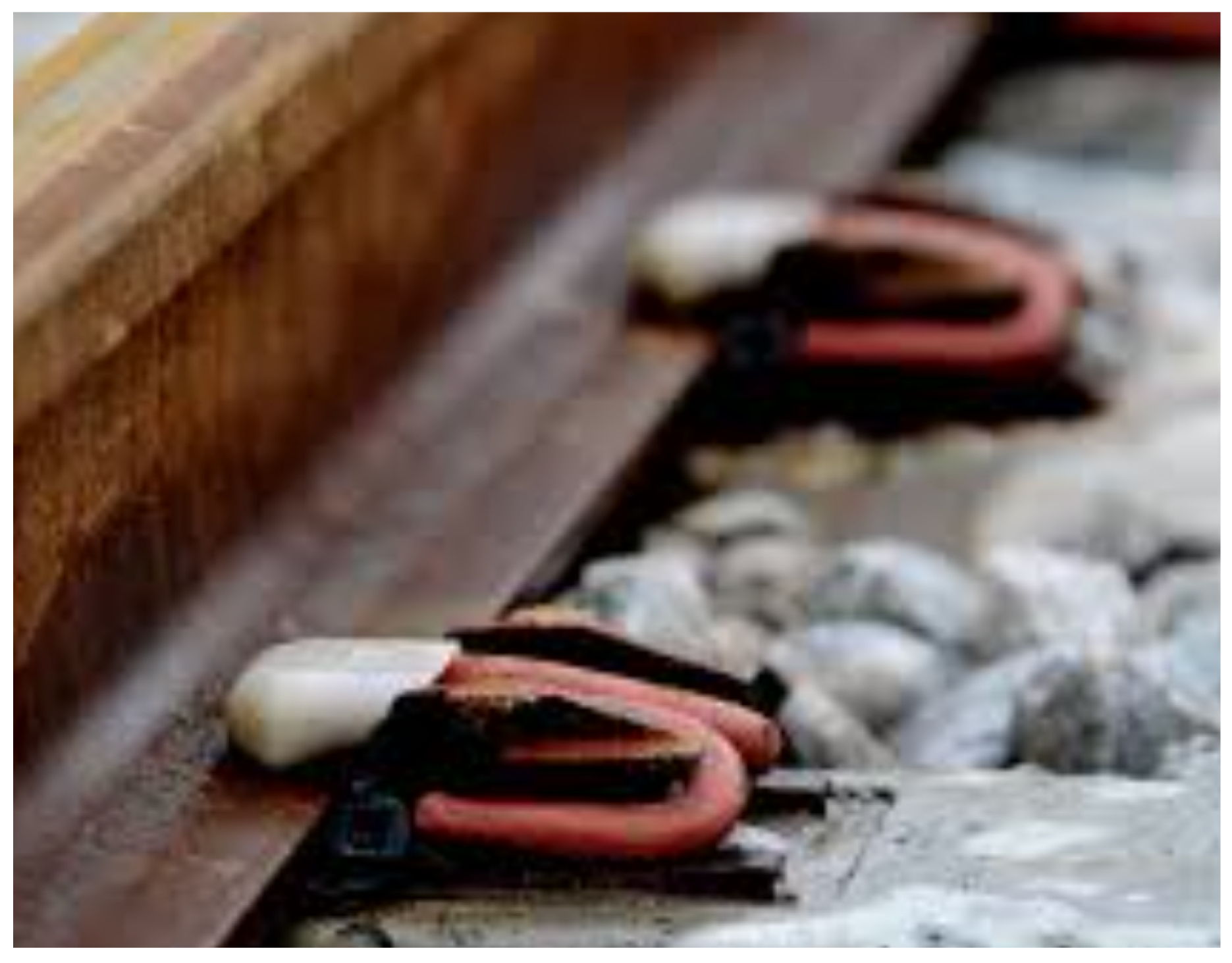
Figure 8.
The image of SFC fastener.
Our system employs semantic segmentation technology, which can assign each pixel in the image to different semantic categories. Compared with traditional object-detection algorithms, semantic segmentation technology can provide more accurate pixel-level segmentation results. Although inaccurate segmentation of pixels may occur in exceptional scenarios, our design ensures that semantic segmentation still produces results. We obtain the final detection results by calculating the target feature values. This approach can effectively reduce the false positive and false negative rates and improve the accuracy and stability of detection. Section 5.1 will introduce the Mask FRCN’s experiment result. In Section 5.2, we show the results of the FIQ weight calculation. In Section 5.3, we exhibit the clustering outcomes for hat line lengths, identifying key metrics that differentiate normal from abnormal fasteners. Section 5.4 narrows down on the left hat and shim lengths, establishing a norm and outlier threshold. Section 5.5 parallels this with the right-side analysis, further refining our detection criteria. Section 5.6 concludes the cluster analysis series by examining the shim’s rectangle dimensions, offering a complete dimensional overview of fastener integrity. Section 5.7 culminates in the final experiment result, showcasing the superior performance of our method against traditional object detectors.
5.1. Training of Mask FRCN
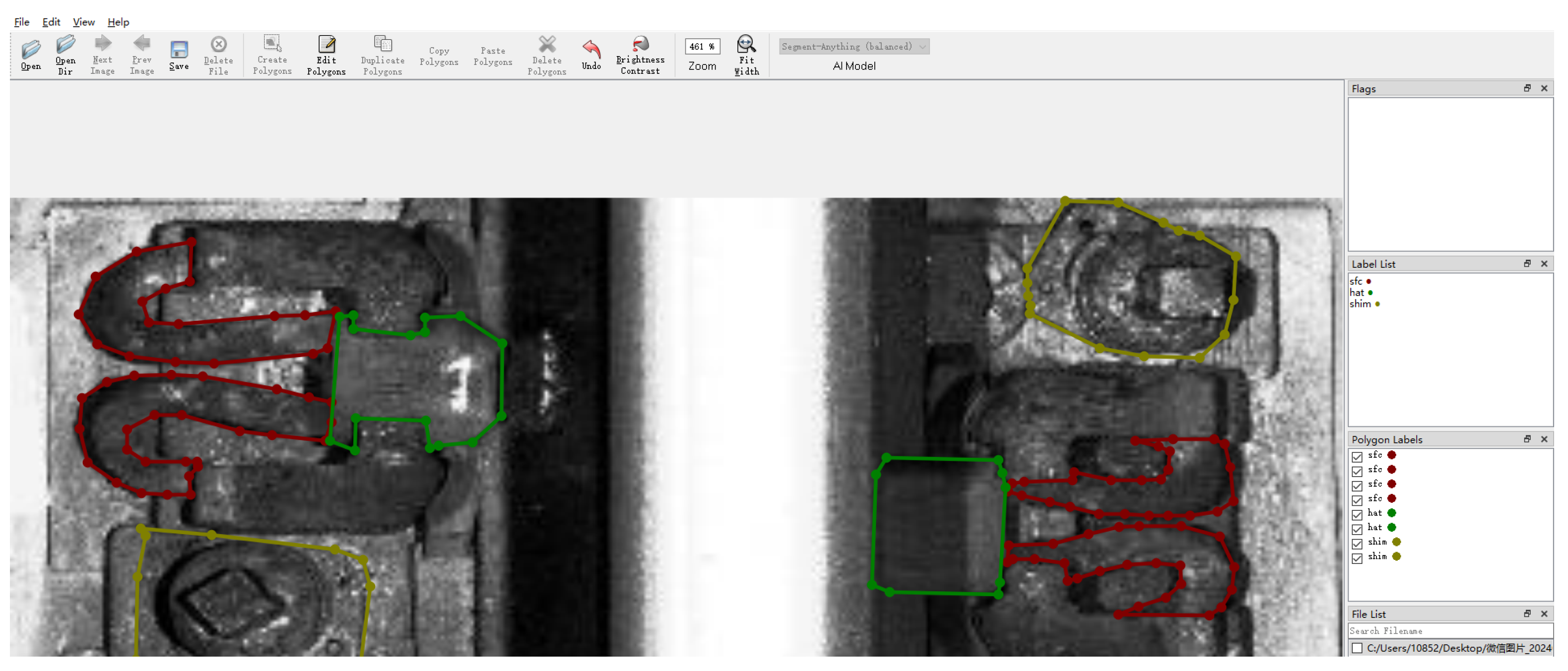
The dataset comprises 900 images of the SFC fastener, captured using two-line scan cameras. The images were split into training, validation, and test sets in a 7:2:1 ratio. Detailed manual annotations were conducted on the training and validation sets using the Labelme platform, ensuring high quality and utility of the dataset shown in Figure 9.

Figure 9.
Annotation screen.
The experimental environment is critical for the segmentation of SFC clip images. As detailed in Table 5, the setup employed a Linux Ubuntu 20.04 OS with an NVIDIA 3080 GPU (Santa Clara, CA, USA), providing robust computational support. Python 1.9.0 and PyTorch 1.11.0 ensured a cutting-edge and stable development environment, whereas 16 GB of RAM facilitated the smooth handling of large-scale data processing and model training.
Table 5.
Detail information of training environment.
The Mask RCNN model was optimized using CWD distillation, incorporating FCRM and FRCN modules. An adaptive learning rate adjustment strategy and early stopping mechanism were implemented. The initial learning rate was set to 0.001 and adjusted based on the validation set performance. Early stopping was triggered when validation performance plateaued. During CWD distillation, the temperature parameter was set to 2, and distillation weights were adjusted to ensure effective knowledge transfer between teacher and student networks in Table 6. The Mask FRCN experiment result is shown as Table 7 and Figure 10. The FIQ score is shown below as Table 8.
Table 6.
Training parameters for Mask FRCN model with CWD distillation.
Table 7.
Evaluation metrics at Mask FRCN optimization stages.

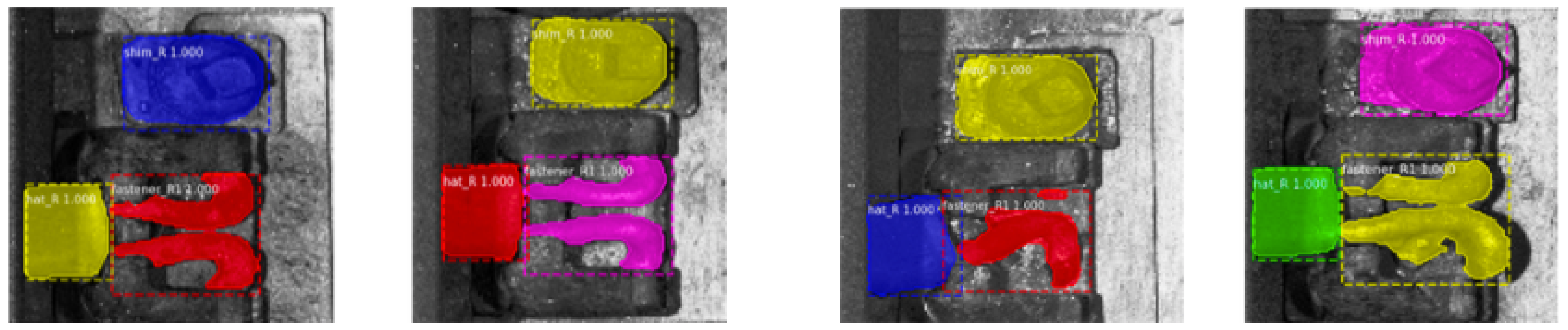
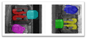
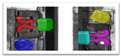
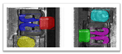
Figure 10.
The predicted result of Mask FRCN.
Table 8.
FIQ score and result.
5.2. Build FIQ Weight Calculation Result
We select 930 sample images as a dataset to obtain FIQ feature weight. The result is in Table 9.
Table 9.
The result of random forest.
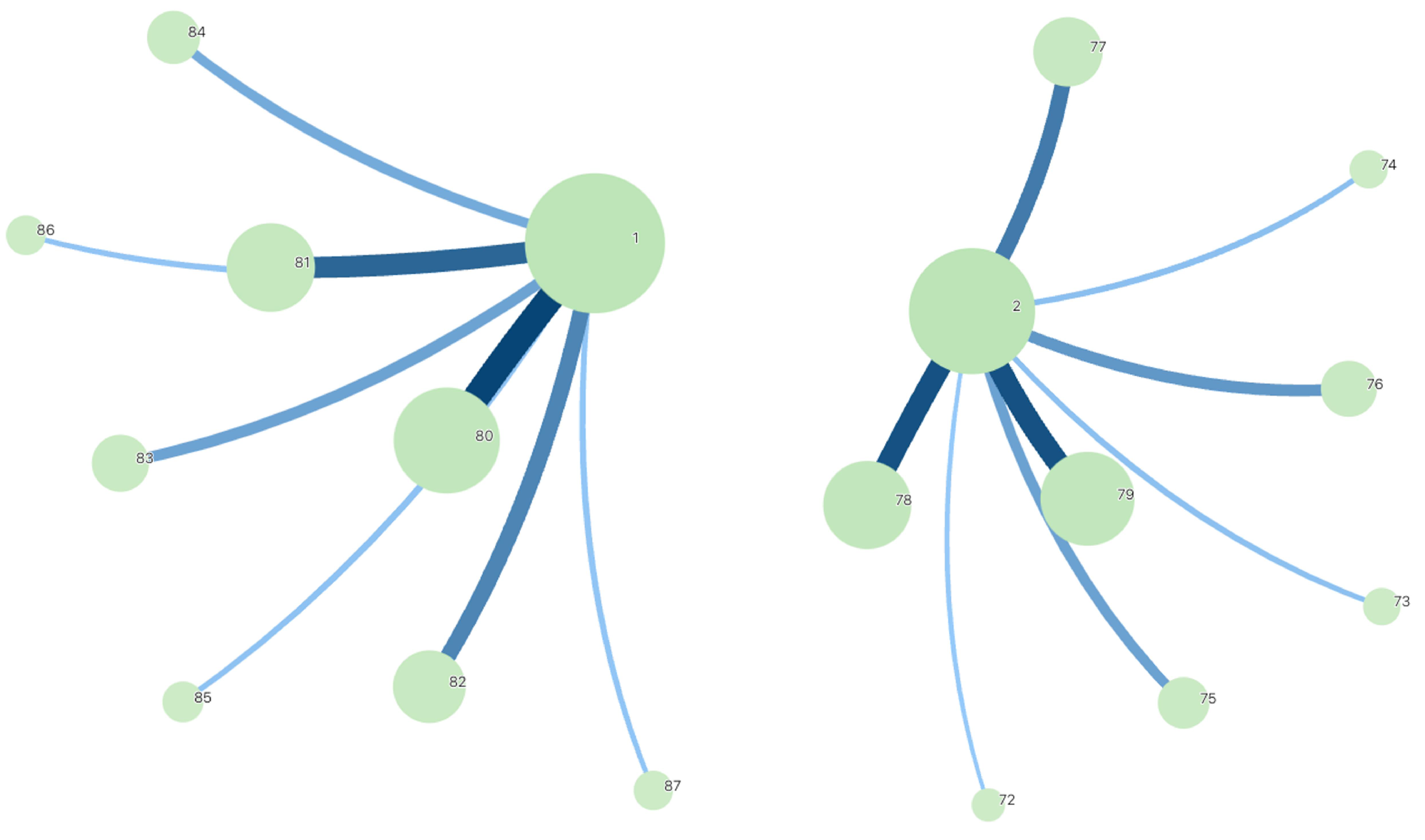
5.3. Cluster Result of Hat Line Length
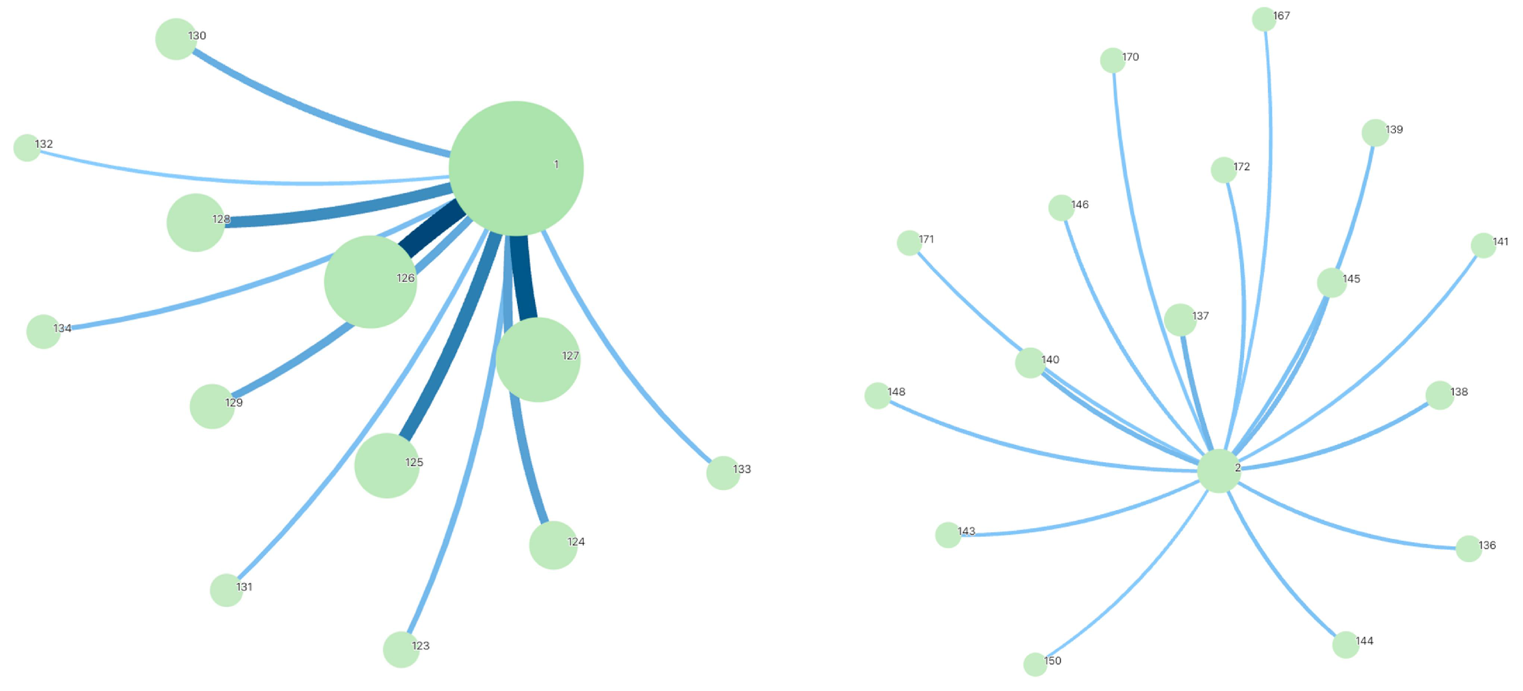
As Table 10 and Figure 11 show, we conducted clustering analysis on the fastener and cap connection lengths of the existing data, and the results are shown in the table below. The mean of normal connection lengths is 127, whereas the outliers are at 145.
Table 10.
The result of hat line length.

Figure 11.
Hat length cluster result. The meaning of this clustering diagram is that the larger the circle, the closer the value, and the thicker the line, the closer the relationship between the two circles.
5.4. Cluster Result of Left Hat and Shim Line Length
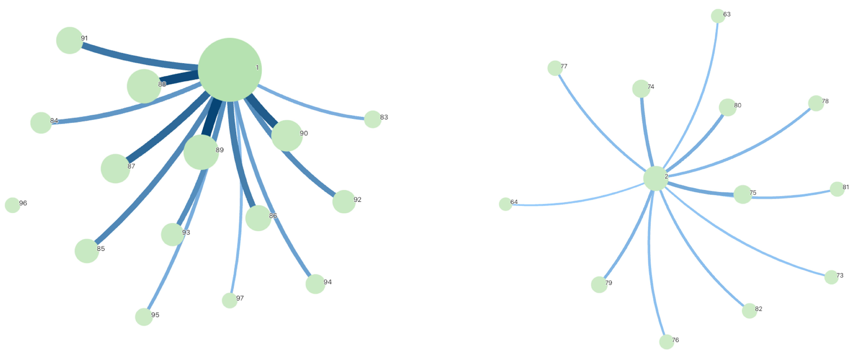
As Table 11, and Figure 12 shows, we conducted clustering analysis on the fastener cap between connection lengths of the existing data, and the results are shown in the table below. The mean of normal connection lengths is 89.55, whereas the outliers are at 76.95.
Table 11.
Cluster result of left hat and shim line length.

Figure 12.
Left hat and shim length cluster result.
5.5. Cluster Result of Right Hat and Shim Line Length
As Table 12 and Figure 13 show, We conducted clustering analysis on the fastener cap and shim connection lengths of the existing data, and the results are shown in the table below. The mean of normal connection lengths is 81.32 and 78.46, whereas the outliers are at 76.95.
Table 12.
Cluster result of right hat and shim line length.

Figure 13.
Right hat and shim length cluster result.
5.6. Cluster Result of Shim’s Recetangle
As Figure 14 shows, we conducted clustering analysis on the length and width of the minimum bounding rectangle of the shim and obtained the mean value.

Figure 14.
Shim cluster result.
5.7. Final Experiment Result
After constructing the FIQ, we obtained the final quantification system for track fasteners. We tested it on a dataset of 350 images, and the experimental results are shown in Table 13 and Table 14. Traditional object-detection algorithms such as SSD [27] and YOLO [28,29] have weak robustness in track fastener scenes, resulting in some failures to detect damaged fasteners. However, our proposed FIQ method can effectively use image segmentation results to calculate an objective evaluation of track fasteners, reducing the current rate of missed detections.
Table 13.
Comparison of experimental results.
Table 14.
The result of different inception methods.
6. Conclusions
In real railway scenarios, the occurrence of abnormal fasteners is significantly lower than that of normal fasteners. Imbalanced datasets can affect the stability and accuracy of inspection models. Therefore, we need an abnormal fastener quantification method to determine whether a fastener needs to be fixed or not. To address this issue, a lightweight high-precision segmentation network and quantification system for track fasteners is proposed. This method first uses MASK-FRCN to segment the foreground clipping area of the fasteners. After obtaining the segmented connected domains, the state of the track fasteners is quantitatively evaluated by our designed FIQ, which obtains evaluation scores and determines the quality and degree of damage of the track fasteners. Experimental results show that this fastener defect detection method performs well on imbalanced datasets, achieving significant accuracy and speed and has strong robustness. This method can be applied to various types of fastener detection tasks and has important theoretical and practical value.
This approach effectively reduces false positives and false negatives, improving the accuracy and stability of detection. Our enhanced Mask-FRCN improves segmentation accuracy to 96.01% and reduces network size to 36.1M. FIQ improves the fault detection accuracy of SFC-type fasteners to 95.13%, highlighting our method’s efficacy and efficiency.
The current study, although presenting a novel approach to fastener inspection, acknowledges the need for further optimization to enhance the model’s accuracy and processing speed, essential for real-time applications. Moreover, this research is recognized to have simplified the analysis by not extensively addressing the complexities of imbalanced samples. Future work will concentrate on refining the model for real-time detection capabilities and expanding the method to include deep learning-based detection of defects in WJ-7 fasteners, thereby tackling the limitations of imbalanced datasets more effectively.
Author Contributions
L.L., Z.S. and S.Z.; data collection: Z.S. and L.L.; analysis and interpretation of results: Z.S. and Y.M.; draft manuscript preparation: Z.S., S.Z. and R.S. All authors reviewed the results and approved the final version of the manuscript.
Funding
This work was supported in part by the National Natural Science Foundation of China (Grant Nos. 51975347 and 51907117) and in part by the Shanghai Science and Technology Program (Grant No. 22010501600).
Data Availability Statement
The raw data supporting the conclusions of this article will be made available by the authors on request.
Acknowledgments
The authors wish to express sincere appreciation to the reviewers for their valuable comments, which significantly improved this paper. The authors would like to give thanks to the Shanghai University of Engineering Science, for promoting this research and providing the laboratory facility and support.
Conflicts of Interest
The authors declare that they have no conflicts of interest to report regarding the present study.
References
- Xia, Y.; Gao, L.; Zhang, J.; Liu, Y. Fastener detection in high-speed railway based on Adaboost cascade classifier. J. Signal Inf. Process. 2013, 4, 337–342. [Google Scholar]
- Feng, J.; Chen, Z.; Wang, Y. Fast detection of railway track fastener defects based on Haar-like features. Signal Process. 2013, 93, 2812–2823. [Google Scholar]
- Yuan, Z.; Zhu, S. Vibration-based damage detection of rail fastener clip using convolutional neural network: Experiment and simulation. Eng. Fail. Anal. 2021, 119, 104906. [Google Scholar] [CrossRef]
- Liu, J.; Liu, H. Cascade Learning Embedded Vision Inspection of Rail Fastener by Using a Fault Detection IoT Vehicle. IEEE Internet Things J. 2023, 10, 3006–3017. [Google Scholar] [CrossRef]
- Wei, X.; Wei, D.; Suo, D.; Jia, L.; Li, Y. Multi-target defect identification for railway track line based on image processing and improved YOLOv3 model. IEEE Access 2020, 8, 61973–61988. [Google Scholar] [CrossRef]
- Wang, J.; Li, L.M.; Zheng, S.B.; Zhao, S.G.; Chai, X.D. A detection method of bolts on axle box cover based on cascade deep convolutional neural network. Comput. Model. Eng. Sci. 2022, 134, 1671–1706. [Google Scholar]
- Ling, X.; Chen, L.; Xiao, J.; Yuan, Y. A hierarchical features-based railway fastener detection method. IEEE Trans. Instrum. Meas. 2020, 69, 7580–7590. [Google Scholar]
- Liu, F.; Zhu, Z.; Feng, J. Railway fastener detection using deep learning. In Proceedings of the International Conference on Intelligent Transportation Systems, ITSC 2018, Maui, HI, USA, 4–7 November 2018; pp. 2605–2609. [Google Scholar]
- Zheng, D.Y.; Li, L.M.; Zheng, S.B.; Chai, X.D.; Zhao, S.G. A defect detection method for rail surface and fasteners based on deep convolutional neural network. Comput. Intell. Neurosci. 2021, 2021, 2565500. [Google Scholar] [CrossRef] [PubMed]
- Liu, J.; Liu, F.; Feng, J. Railway fastener detection based on U-Net and GANs. In Proceedings of the International Conference on Intelligent Transportation Systems (ITSC 2019), Auckland, New Zealand, 27–30 October 2019; pp. 3392–3396. [Google Scholar]
- Goodfellow, I.; Pouget-Abadie, J.; Mirza, M.; Xu, B.; Warde-Farley, D.; Ozair, S.; Bengio, Y. Generative adversarial nets. Adv. Neural Inf. Process. Syst. 2014, 27, 2672–2680. [Google Scholar]
- Su, S.; Du, S. RFS-Net: Railway Track Fastener Segmentation Network with Shape Guidance. IEEE Trans. Circuits Syst. Video Technol. 2023, 33, 1398–1412. [Google Scholar] [CrossRef]
- Muhammad, O.; Hussain, I. Railway Track Joints and Fasteners Fault Detection using Principal Component Analysis. In Proceedings of the International Conference on Robotics and Automation (ICRA 2023), London, UK, 29 May–2 June 2023; pp. 1–6. [Google Scholar]
- Liu, J.; Huang, Y.; Wang, S.; Zhao, X.; Zou, Q. Rail fastener defect inspection method for multi railways based on machine vision. Railw. Sci. 2022, 1, 210–223. [Google Scholar] [CrossRef]
- Chandran, P.; Asber, J.; Thiery, F.; Odelius, J.; Rantatalo, M. An investigation of railway fastener detection using image processing and augmented deep learning. Sustainability 2021, 13, 12051. [Google Scholar] [CrossRef]
- Wei, X.K.; Jiang, S.Y.; Li, Y.; Li, C.L.; Jia, L.M. Defect detection of pantograph slide based on deep learning and image processing technology. IEEE Trans. Intell. Transp. Syst. 2021, 21, 947–958. [Google Scholar] [CrossRef]
- Kim, B.; Jeon, Y. Multi-task Transfer Learning Facilitated by Segmentation and Denoising for Anomaly Detection of Rail Fasteners. J. Electr. Eng. Technol. 2023, 18, 2383–2394. [Google Scholar] [CrossRef]
- Wei, W.; Cai, Z.; Zhang, Z. Railway fastener detection based on Faster-RCNN and YOLO V3. IOP Conf. Ser. Mater. Sci. Eng. 2019, 569, 042060. [Google Scholar]
- Wang, H.; Wang, Z.; Liu, Z. Railway fastener detection method based on improved Faster R-CNN. In Proceedings of the International Conference on Control, Automation and Robotics (ICCAR 2019), Beijing, China, 19–22 April 2019; pp. 580–584. [Google Scholar]
- Zhang, S.; Wen, L.; Bian, X.; Lei, Z.; Li, S.Z. Single-shot object detection with enriched semantics. In Proceedings of the IEEE/CVF Conference on Computer Vision and Pattern Recognition (CVPR 2018), Salt Lake City, UT, USA, 18–22 June 2018; pp. 5813–5821. [Google Scholar]
- He, K.; Gkioxari, G.; Dollár, P.; Girshick, R. Mask R-CNN. In Proceedings of the 2017 IEEE International Conference on Computer Vision (ICCV 2017), Venice, Italy, 22–29 October 2017; pp. 2961–2969. [Google Scholar]
- He, K.; Zhang, X.; Ren, S.; Sun, J. Deep residual learning for image recognition. In Proceedings of the 2016 IEEE Conference on Computer Vision and Pattern Recognition (CVPR), Las Vegas, NV, USA, 27–30 June 2016; pp. 770–778. [Google Scholar]
- Park, W.; Kim, D.; Lu, Y.; Cho, M. Relational Knowledge Distillation. In Proceedings of the 2020 IEEE/CVF Conference on Computer Vision and Pattern Recognition, CVPR Workshops 2020, Seattle, WA, USA, 14–19 June 2020; pp. 5957–5966. [Google Scholar]
- Hu, J.; Shen, L.; Sun, G. Squeeze-and-Excitation Networks. In Proceedings of the 2018 IEEE Conference on Computer Vision and Pattern Recognition Workshops, CVPR Workshops 2018, Salt Lake City, UT, USA, 18–22 June 2018; pp. 7132–7141. [Google Scholar]
- Frosst, N.; Hinton, G. Distilling a Neural Network Into a Soft Decision Tree. arXiv 2017, arXiv:1711.09784. [Google Scholar]
- Woo, S.; Park, J.; Lee, J.-Y.; Kweon, I.S. CBAM: Convolutional Block Attention Module. In Proceedings of the European Conference on Computer Vision (ECCV), Munich, Germany, 8–14 September 2018; pp. 3–19. [Google Scholar]
- Liu, W.; Anguelov, D.; Erhan, D.; Szegedy, C.; Reed, S.; Fu, C.-Y.; Berg, A.C. SSD: Single Shot MultiBox Detector. In Proceedings of the Computer Vision—ECCV 2016: 14th European Conference, Amsterdam, The Netherlands, 11–14 October 2016; pp. 21–37. [Google Scholar]
- Redmon, J.; Farhadi, A. YOLOv3: An Incremental Improvement. arXiv 2018, arXiv:1804.02767. [Google Scholar]
- Bochkovskiy, A.; Wang, C.-Y.; Liao, H.-Y.M. YOLOv5: Optimal Speed and Accuracy of Object Detection. arXiv 2021, arXiv:2004.10934. [Google Scholar]


Disclaimer/Publisher’s Note: The statements, opinions and data contained in all publications are solely those of the individual author(s) and contributor(s) and not of MDPI and/or the editor(s). MDPI and/or the editor(s) disclaim responsibility for any injury to people or property resulting from any ideas, methods, instructions or products referred to in the content. |
© 2024 by the authors. Licensee MDPI, Basel, Switzerland. This article is an open access article distributed under the terms and conditions of the Creative Commons Attribution (CC BY) license (https://creativecommons.org/licenses/by/4.0/).