Abstract
This paper proposes a dead-reckoning (DR) method for vehicles using Lie theory. This approach treats the pose (position and attitude) and velocity of the vehicle as elements of the Lie group and follows the computations based on Lie theory. Previously employed DR methods, which have been widely used, suffer from cumulative errors over time due to inaccuracies in the calculated changes from velocity during the motion of the vehicle or small errors in modeling assumptions. Consequently, this results in significant discrepancies between the estimated and actual positions over time. However, by treating the pose and velocity of the vehicle as elements of the Lie group, the proposed method allows for accurate solutions without the errors introduced by linearization. The incremental updates for pose and velocity in the DR computation are represented in the Lie algebra. Experimental results confirm that the proposed method improves the accuracy of DR. In particular, as the motion prediction time interval of the vehicle increases, the proposed method demonstrates a more pronounced improvement in positional accuracy.
1. Introduction
In the realm of pose (position and attitude) estimation, dead-reckoning (DR) plays a pivotal role, particularly in Kalman filter (KF)-based methods where it is utilized during the prediction stage. The accuracy of DR is paramount in improving the performance of pose estimation algorithms. As DR is employed to forecast the future state of a vehicle based on its current state and motion dynamics, any inaccuracies in DR computations can significantly impact the accuracy of the estimation process. Therefore, ensuring precise DR calculations is essential to enhance the overall estimation performance [1,2,3,4]. However, most previously used DR approaches are prone to errors due to inevitable approximations in numerical integration and approximations in attitude-related operations. In other words, they face issues such as decreasing accuracy of position with increasing time of numerical integration and problems in handling attitude and rotation operations in Cartesian space.
DR involves predicting the position and attitude of a vehicle through integration, which introduces approximation errors due to sensor-measured data integration over the motion prediction time [5]. These errors accumulate over time, leading to significant discrepancies between the predicted and actual poses [6,7]. Although shorter prediction time intervals may reduce errors, precision is not guaranteed. Consequently, implementing DR with approximate integration decreases prediction accuracy and increases uncertainty, especially in recursive filters like the KF. Additionally, as the prediction cycle of the vehicle increases, the method’s accuracy diminishes, making it unsuitable for position prediction with long velocity measurement cycles. Therefore, ensuring precise DR calculations is essential to enhance the overall prediction performance.
The rotation and attitude of a vehicle cannot be perfectly represented and computed within the linear space of Cartesian coordinates [8,9]. When the attitude is approximated and calculated within this linear space, errors due to approximation arise, leading to a decrease in position accuracy. Numerous researchers have assumed that attitudes, represented by Euler angles, form a linear space and have performed calculations based on this assumption. However, Euler angles can lead to gimbal lock, where a particular rotation axis becomes aligned with another axis [10,11]. Euler angles indeed encounter difficulties in accurately representing all attitudes, particularly when the pitch axis nears ±90 degrees, thereby complicating processing and representation tasks [12,13]. However, when it comes to DR, the challenges are more nuanced and stem from the limitations of Euler angles in expressing and operating rotations. Specifically, the use of Euler angles introduces singularities, such as gimbal lock, which can disrupt the continuity of orientation measurements and lead to inaccuracies in pose estimation during DR calculations. Furthermore, the nonlinear nature of Euler angle transformations complicates the integration process, making it susceptible to cumulative errors over time. These issues highlight the inadequacy of Euler angles in robustly representing motion dynamics, particularly in dynamic environments where precise pose estimation is crucial for navigation and localization tasks. The primary limitation of previously used DR methods stems from approximating the motion of the vehicle during a single sampling period as linear, leading to errors in position calculation. Another significant issue arises from the linear piecewise approximation of the continuous and coupled changes in pose, which introduces uncertainties. These uncertainties include errors resulting from simply integrating angular rates to estimate changes in attitude, the assumption of attitudes forming a linear space, and the occurrence of gimbal lock.
Research aimed at minimizing cumulative errors to enhance the accuracy of DR is actively being conducted across various fields [14,15,16,17,18]. Shurin et al. (2022) proposed pedestrian DR to address the drift issue over time caused by errors and noise in inertial sensor measurements in the navigation of quadcopters [14]. Jang et al. (2024) developed a position and direction estimation algorithm for active driving of wheelchairs using ultra-wideband (UWB) sensors [15]. Zhang et al. (2023) proposed an accurate underwater DR mathematical model based on the motion model of autonomous underwater vehicles (AUVs) to recursively compute ground truth and associated errors [16]. Bai et al. (2023) proposed a method for tracking upper limb segments using a single inertial sensor to reduce drift in DR-based position tracking [17]. Cao et al. (2023) proposed a DR method using only wheel speeds to achieve accurate path tracking in extreme situations where location sensors are absent [18].
To further enhance the robustness and accuracy of DR systems, recent studies have explored the integration of factor graphs [19,20]. Zhang et al. (2024) optimized AUV navigation by integrating side-scan sonar (SSS) data and inertial measurement units (IMU) using factor graphs, demonstrating significant improvements in positioning accuracy under challenging conditions [19]. Similarly, Ma et al. (2021) developed a multi-source information fusion algorithm based on factor graphs for AUVs, achieving enhanced computational efficiency and navigation performance by processing asynchronous heterogeneous measurements [20]. Additionally, information geometry has been employed to optimize navigation algorithms by enhancing their robustness and accuracy [21,22]. Shahoud et al. (2022) utilized street geometry information to improve visual navigation and path tracking for drones. This approach compensated for visual odometry drift through scene matching and servo control, leveraging known street geometries to enhance the precision of image alignment [21]. Moreover, information geometry principles have been applied to improve unmanned aerial vehicle (UAV) circular control by optimizing Fisher information, thus enhancing the stability and accuracy of the navigation system [22]. These advanced approaches address the limitations of traditional methods by effectively handling attitude and rotation in nonlinear spaces and reducing numerical approximation errors.
To overcome these limitations, this paper proposes a DR approach by representing the pose and velocity of the vehicle in the three-dimensional special Euclidean group, an extended Lie group ((3)), based on Lie theory [23,24,25]. The proposed method resolves the approximation error issue of previously used DR by computing the attitude of objects moving in nonlinear spaces. Additionally, as the attitude of the vehicle is also represented by the Lie group, the 3D special orthogonal group (SO(3)), there is no need to approximate the attitude in a linear space, thus addressing the issue of model uncertainty concerning attitude. Lie theory-based DR handles the integration of the attitude of vehicles accurately and without approximation, significantly reducing the influence of time intervals compared to previously used DR methods [26,27]. Constructing the state as a Lie group in Lie theory-based DR provides highly accurate spatial representations, overcoming the limitations of previously used DR methods and achieving improved performance in terms of accuracy, consistency, and stability.
The main contributions and novel aspects of this study can be summarized as follows:
- Enhanced Accuracy in Pose Prediction: The proposed method significantly improves the accuracy of pose prediction for vehicle motion. By employing Lie theory-based methods, the approach enables rigorous DR calculations without approximations, precisely modeling translations and rotations, especially in three-dimensional space. This results in more accurate vehicle pose determination.
- Elimination of Linear Space Assumptions: Utilizing Lie groups, the method eliminates the necessity to assume that vehicle rotation or attitude forms a linear space. This avoids the need to force rotations or attitudes into a linear space, thereby preventing the introduction of approximation errors and enhancing overall prediction accuracy.
- Reduction of Cumulative Approximation Errors: The proposed method addresses and overcomes the limitations of conventional DR methods that suffer from cumulative approximation errors in integration operations. These errors are typically caused by inaccuracies in linear and angular velocity measurements, motion prediction time intervals, and computational limitations. By performing accurate computations in nonlinear spaces, the proposed method effectively reduces these cumulative errors, enhancing the overall estimation accuracy.
- Application in Pose Estimation Algorithms: The method can be seamlessly integrated as a process model in pose estimation algorithms, such as the KF. It provides highly accurate predictions of the current state during the prediction phase, thereby reducing estimation uncertainty and improving the robustness and reliability of the estimation process.
The significance of the results can be highlighted as follows:
- The results demonstrate a substantial improvement in the accuracy and reliability of vehicle pose prediction.
- The proposed method’s ability to mitigate cumulative errors and operate effectively in nonlinear spaces highlights its potential for practical applications in autonomous driving and other related fields.
- The findings suggest that adopting this method can lead to more precise and dependable navigation systems, ultimately contributing to the advancement of autonomous vehicle technologies.
- This novel approach not only enhances the theoretical foundation of vehicle pose estimation but also provides a practical solution that can be directly implemented in real-world autonomous systems.
- The method offers significant benefits in terms of performance and reliability, making it a valuable contribution to the field of autonomous driving.
In Section 2, we provide an overview of the previous DR methods commonly used and discuss their limitations. Section 3 presents an overview of the theoretical background, Lie theory, and describes the Lie theory-based DR method. Section 4 illustrates how the proposed method outperforms previously used methods using experimental results obtained from real-world data. Finally, in Section 5, we summarize the research findings and present future research directions.
2. Limitation of Previously Used Dead-Reckoning Approach
In this section, we describe the previously widely used DR approaches and discuss their limitations.
The state at time t consists of the position , velocity , and attitude as follows:
In Equation (1), the position and velocity of the vehicle belong to a three-dimensional real vector space. Both position and velocity are described in the east-north-up (ENU) coordinate frame.
The attitude is expressed as Euler angles as follows:
Previously widely used DR predicts the pose and velocity of a vehicle through a motion model from the state and the measured input as follows:
where f(·) denotes a time-varying nonlinear function, and is the process noise. The expression is the measured input and is expressed as follows:
In Equation (6), is the linear velocity of the vehicle, is the acceleration of the vehicle, and is the angular velocity of the vehicle.
The position, velocity, and attitude of the vehicle at the th time step can be calculated as follows:
Equation (7) is rephrased as
The change in position, , is calculated from the rotation matrix (), linear velocity (), and the data reception period ().
where is . In Equation (9), the linear velocity is the linear velocity in the body frame of the vehicle, so the coordinate transformation is performed to the ENU coordinate frame through the rotation matrix. The rotation matrix is expressed from the attitude of the vehicle as follows:
where
The change in velocity, , is calculated from the acceleration and . However, because the acceleration is the acceleration in the body frame of the vehicle, the coordinate transformation to the ENU coordinate frame must be performed as follows:
The attitude change vector is calculated using the angular velocity vector . This expresses the relationship between angular velocity and attitude, modeling the time variation of attitude. The connection between angular velocity and attitude change is represented by the derivative of the rotation matrix with respect to the Euler angles.
The previous method corresponds to a first-order approximation.
Here, Equations (9), (11) and (12) correspond to for position, velocity, and attitude, respectively.
Previously widely used DR inevitably leads to errors between the measured discrete rotation values and the actual continuous rotation values due to approximate integration. This is because the approximate integration error in the time interval accumulates, causing a drift phenomenon. As the integration error accumulates, it becomes difficult to accurately calculate the attitude as the dynamic movement time of the vehicle increases, leading to a decrease in position prediction accuracy. Additionally, since the attitude is forcibly approximated and expressed in a linear space, errors due to approximation occur, leading to a decrease in accuracy for position.
3. Lie Theory-Based Dead-Reckoning Approach
In this section, we propose a Lie theory-based DR to overcome the limitations mentioned in Section 2. The measured input is the same as in Section 2.
3.1. Lie Theory Tools for Dead-Reckoning
To overcome the limitations of previously widely used DR methods, this paper introduces Lie theory. The introduced Lie theory includes theories related to physical roles according to the concepts of Lie groups and Lie algebras.
Lie groups are used to represent continuous transformations in DR systems. The position, velocity, and attitude of a vehicle are expressed as elements of a Lie group, and these elements are used to change over time and perform various transformations. Lie groups are also important tools for understanding the symmetry of DR systems, allowing for the study and analysis of transformations performed by the system. Lie groups are one of the key concepts in algebraic structure and differential geometry. Mathematically, it is a special set that is both a group and a smooth manifold. The concept of a smooth manifold is related to differential geometry, and the smoothness of a Lie group means that the operation between transformations is differentiable. Commonly used Lie groups in robotics include the n-dimensional special orthogonal group () [28], which represents rotation transformations, the n-dimensional special unitary group (), which plays an important role in quantum mechanics, and the special Euclidean group (), which represents rotations and translations in three-dimensional space [29,30,31]. In addition, there is extended from for rigid body transformations related to transformations or kinematic changes [26,32,33,34].
Lie algebra is an important mathematical structure connected to Lie groups. Whereas Lie groups are special sets that are algebraically smooth and at the same time smooth manifolds, Lie algebras are algebraic objects that represent transformations around the identity element of the corresponding group. Lie algebras are used to provide information about small changes in Lie groups. Therefore, small dynamic changes or errors of a vehicle can be expressed as elements of a Lie algebra. Lie algebras are mainly defined as the tangent space of a Lie group, that is, the tangent space near the identity element of the group. In particular, Lie algebras representing small transformations in Lie groups are mainly expressed as a set of skew-symmetric matrices. Therefore, they are expressed as a set of matrices that satisfy . The size of the matrix depends on the dimension of the Lie group.
Therefore, in Lie theory-based DR, Lie groups and Lie algebras act as important tools for modeling the pose and velocity of vehicles and understanding transformations. These concepts are essential in the design and improvement of DR algorithms and play an important role in improving accuracy and stability. Additionally, Lie theory-based DR performs calculations for rotation and translation of vehicles directly within the Lie group, dividing each rotation into small steps and minimizing approximation errors. In other words, because global optimization is performed through calculations within the Lie group, cumulative errors and approximation errors can be minimized, and accuracy can be maintained.
Figure 1 illustrates the correspondence between Lie groups and Lie algebras and demonstrates the role of the function, a key concept within Lie theory. The function enables the mapping of elements from the Lie algebra to elements of the Lie group. If represents a point on the Lie group (), the velocity at this point () belongs to the tangent space of the Lie group at that point. The structure of this tangent space is consistently maintained throughout the manifold due to its natural smoothness. Notably, the tangent space at the identity element of the group corresponds to the Lie algebra (). Elements within the Lie algebra are represented as skew-symmetric matrices. These matrices can be expressed using the operator ^, which converts column vectors into matrices. The exponential map function is employed to ensure a unique transformation from the Lie algebra to the Lie group matrix. This transformation allows for the mapping of elements from the Lie algebra to their corresponding elements in the Lie group.

Figure 1.
Lie theory.
Mathematically expressing the relationship between the Lie group and Lie algebra, let be a Lie group and be the Lie algebra corresponding to the Lie group . The function maps the Lie algebra element to the Lie group element . The expression is defined differently depending on the group [33]. If , then is as follows:
and are calculated as
where , and is an operator that transforms a vector into a skew-symmetric matrix.
3.2. Lie Theory Application for Three-Dimensional Dead-Reckoning of Vehicles
The group is a group extended from for rigid body transformations related to kinematic changes. The DR process in the Lie group is as follows:
In Equation (16), ⊕ is an operator that combines Lie group elements and Lie algebra elements, and the result of the operation belongs to the Lie group. The Lie group is a transformation matrix that constitutes the position, velocity, and attitude of a vehicle in 3D space, and is expressed as follows:
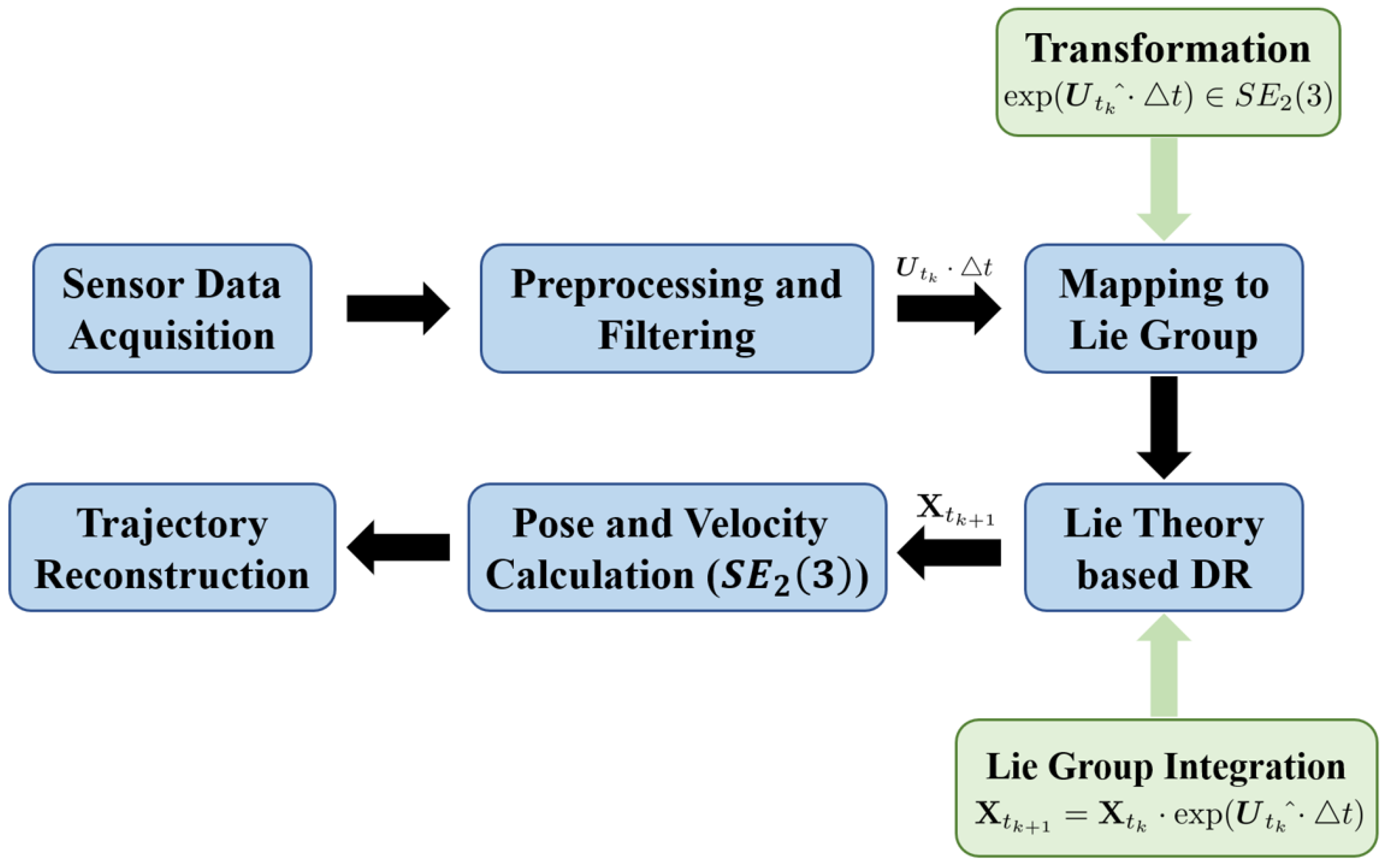
The expressions and also represent the position and velocity of the vehicle in the ENU coordinate frame. The measured input is the same as Equation (6) in Section 2. The expression is calculated from Equation (15). The comprehensive overview of the entire algorithm is presented as a block diagram, as shown in Figure 2.

Figure 2.
Overview of the Lie theory-based dead-reckoning algorithm.
4. Experiments and Results
This section demonstrates the improvements achieved by applying Lie theory through real-world experimental data. The proposed method is compared with the previously widely used DR. The comparison focuses on the accuracy of the prediction results when the sensor data reception cycle is varied. The prediction results refer to the calculated position, velocity, and attitude. Hereafter, the proposed method will be referred to as “proposed”, and “Conv-DR” will represent the previous method, i.e., the previously widely used linear approximation-based DR.
4.1. Experimental Environment
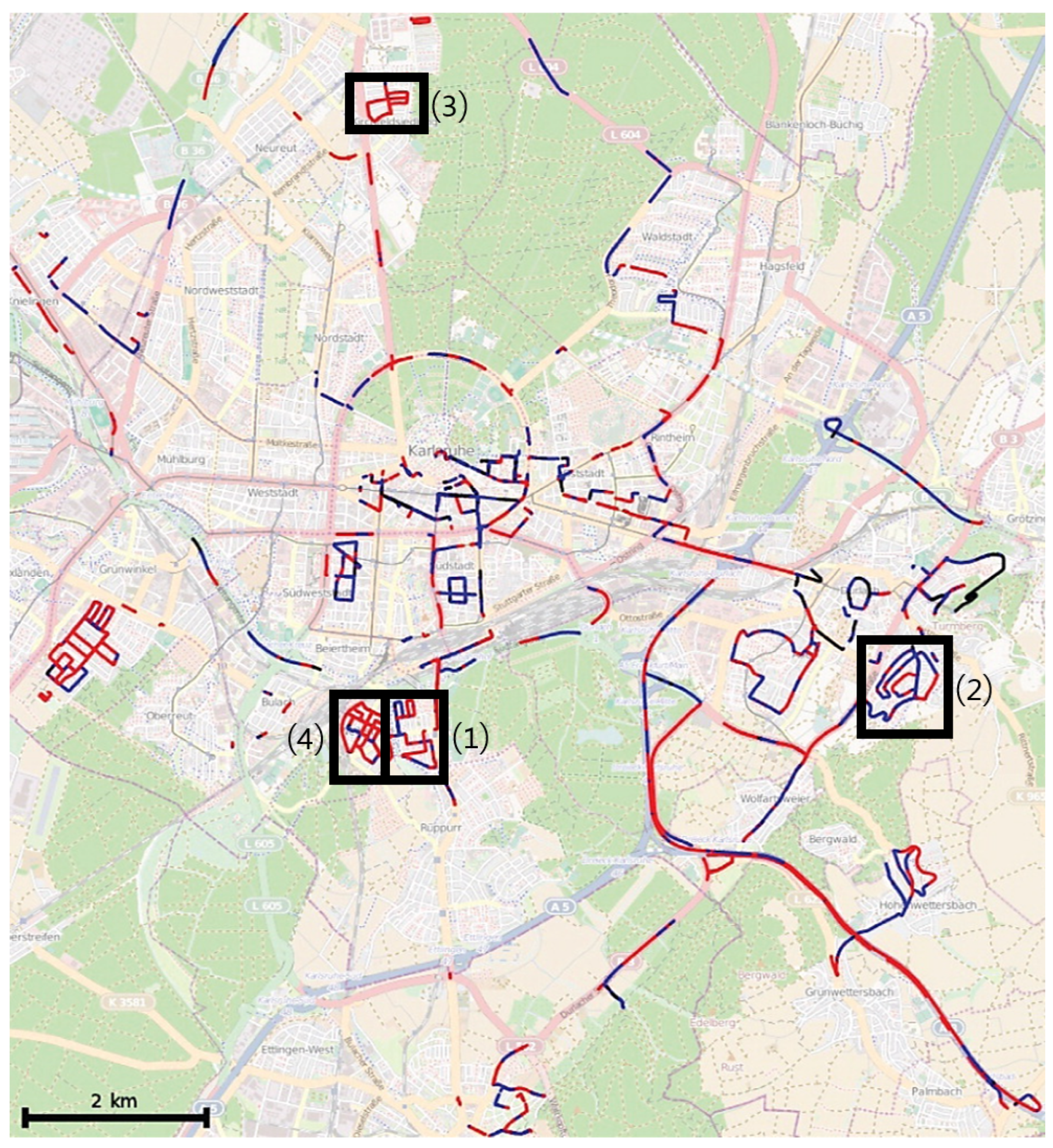
The proposed method was validated using the KITTI dataset, which is widely employed in autonomous driving research by scholars [35]. This dataset captures recordings of vehicle movements in and around Karlsruhe, Germany, incorporating various real-world factors such as noise, drift, and friction. It encompasses camera images, laser scans, precise GPS measurements, and IMU acceleration data collected via a combined GPS/IMU system. Figure 3 shows a map where the colors encode GPS signal quality. The red track is precisely recorded using real time kinematic (RTK)-GPS correction values, the blue track is without correction, and the black track indicates areas excluded from the dataset due to unusable GPS signals.

Figure 3.
Experimental location.
The dataset scenarios provided by [35] are diverse, ranging from highways in rural areas around the medium-sized city of Karlsruhe to urban scenes with many static and dynamic objects. The data used in this paper are from a residential area, characterized by densely packed housing and commercial buildings, narrow roads, numerous intersections, and roadside parking spaces. This data is calibrated, synchronized, and timestamped, and includes both the rectified and raw image sequences. The experiments were conducted during the day.
The vehicle used in the experiments is a VW Passat station wagon modified for autonomous driving research. It is equipped with LiDAR, GPS/IMU, and four video cameras. Our analysis utilized data from four distinct locations, as illustrated in Figure 3, with specifics outlined in Table 1.

Table 1.
Organizing experiment data.
4.2. Position Results
The error of the calculated position in the ENU coordinate frame was compared with the error of the previously used DR. The performance of the method is compared based on the distance error. The distance error indicates the distance between the calculated position and the reference position as shown in Equation (18).
Here, the reference position was obtained using RTK-GPS, which shows the highest accuracy.
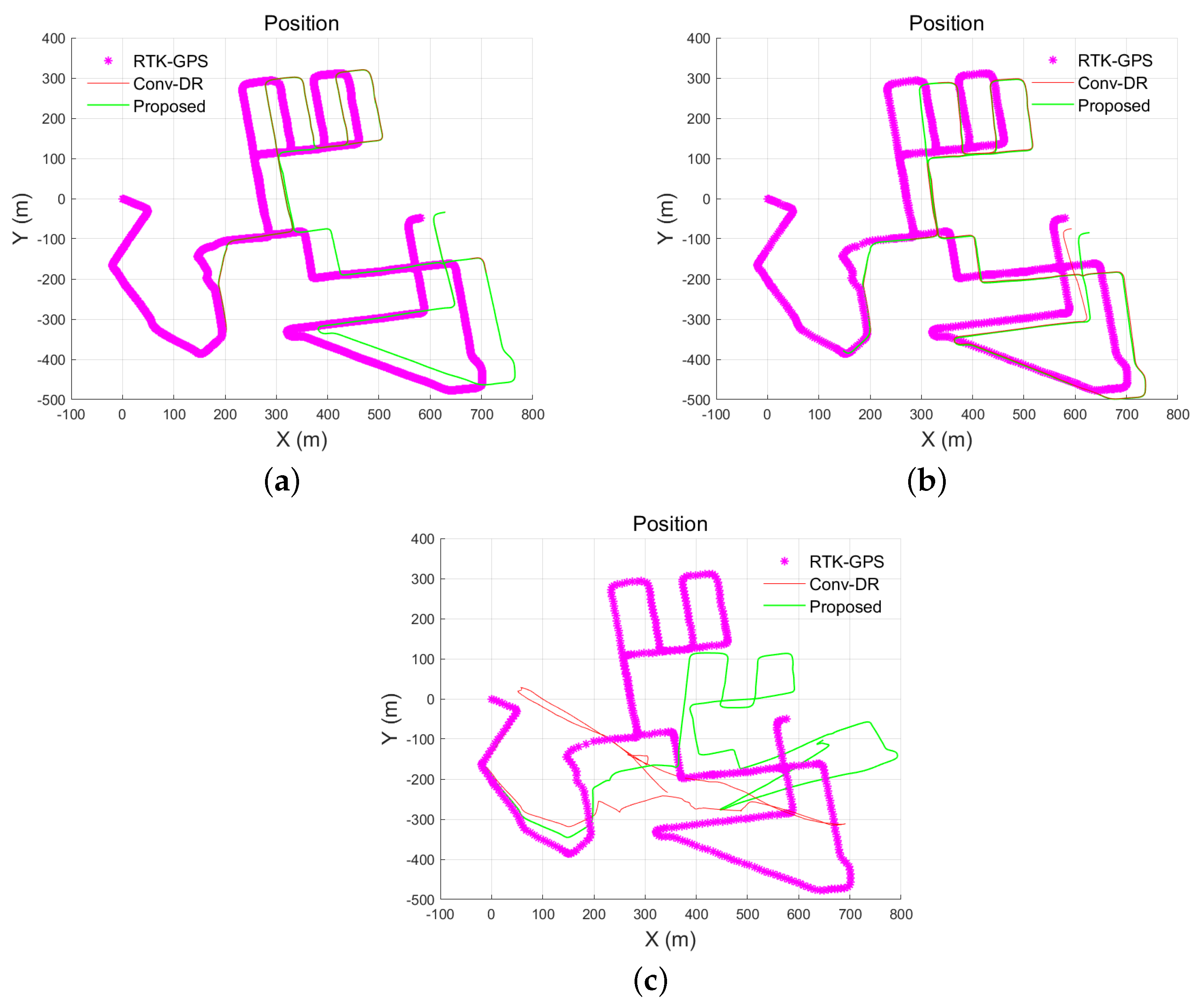
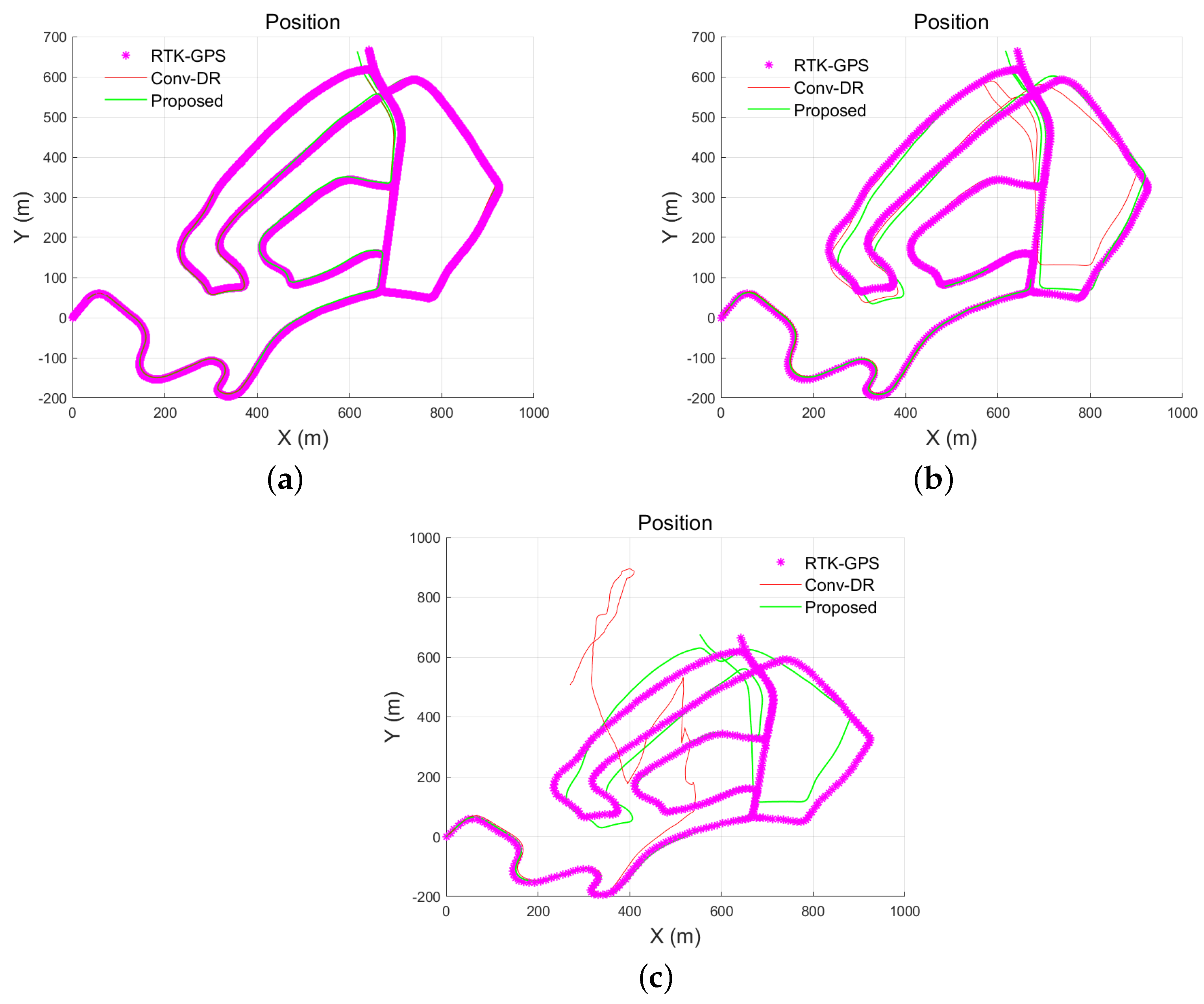
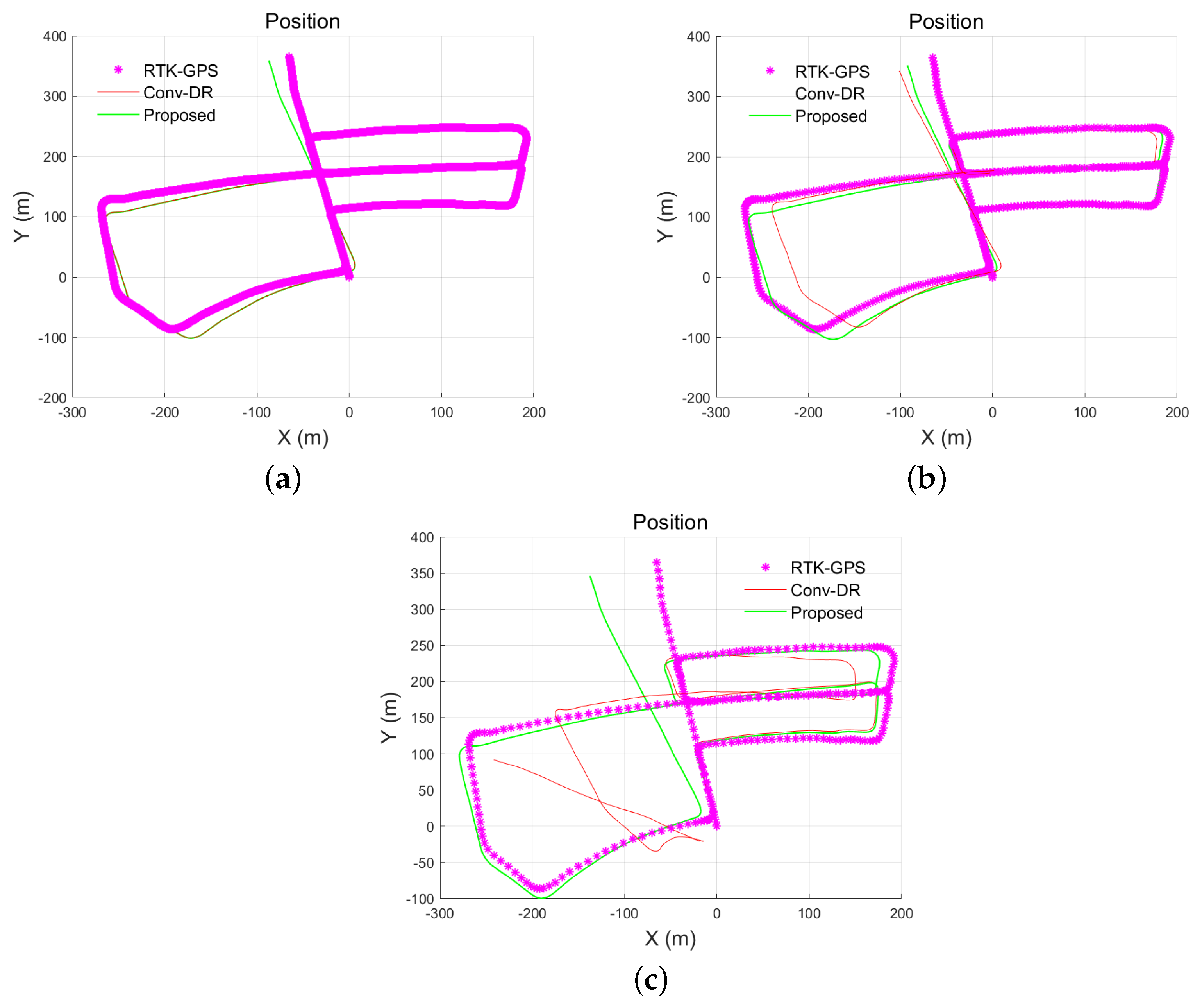
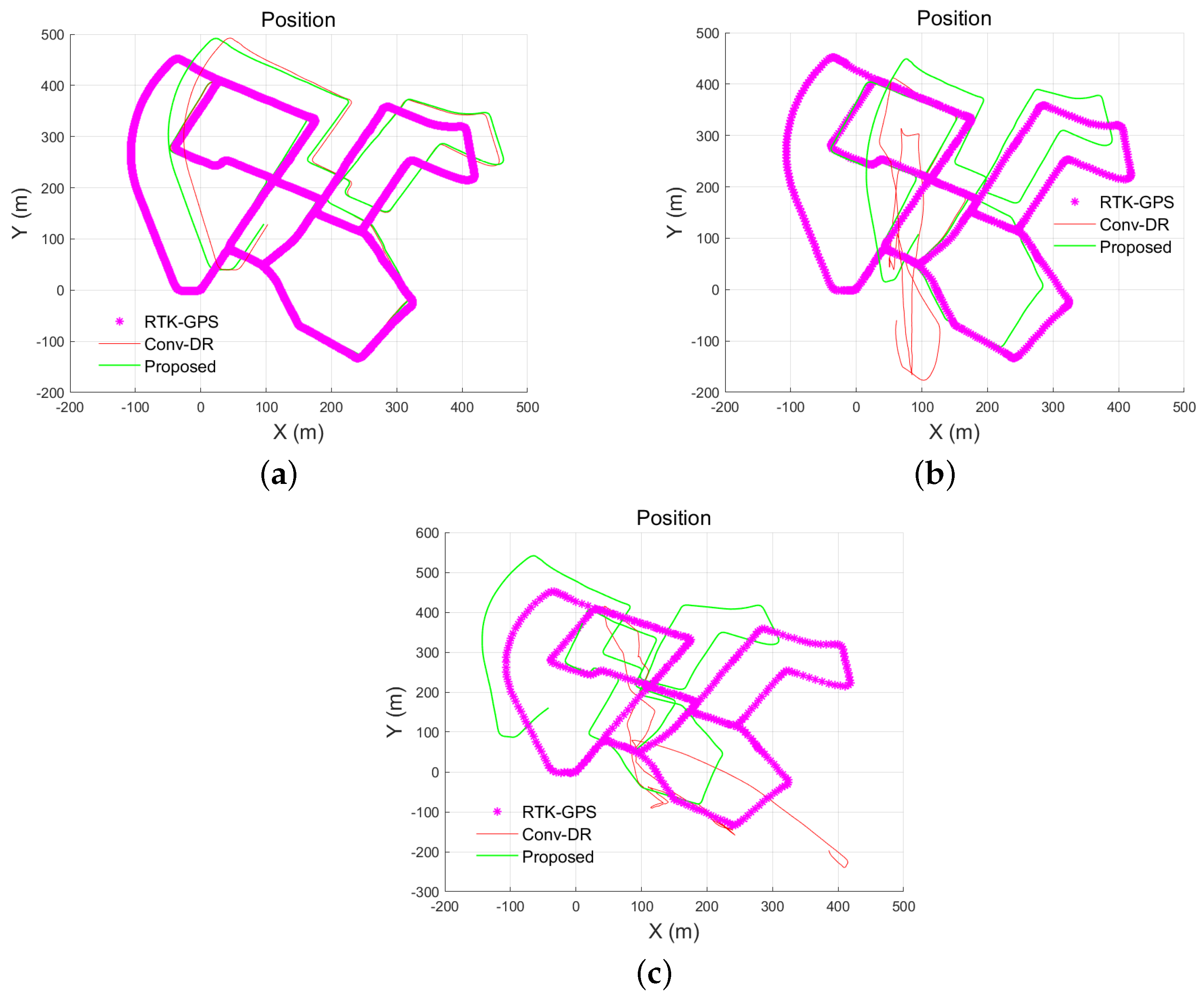
Figure 4, Figure 5, Figure 6 and Figure 7 show the predicted position trajectories on the plane for the experiments conducted in the four regions indicated in Figure 3. The pink graph represents the trajectory measured by RTK-GPS, which is used as the reference in this figure. The red graph indicates the results calculated using the previous method, and the green graph shows the results from the proposed method. In each figure, (a) represents the results when the data reception period is 0.1 s, (b) represents the results for a data reception period of 0.5 s, and (c) represents the results for a data reception period of 1 s.

Figure 4.
Dead-reckoned trajectory calculated by the local data at region (1): (a) has a data reception period of 0.1 s; (b) has a data reception period of 0.5 s; and (c) has a data reception period of 1 s.

Figure 5.
Dead-reckoned trajectory calculated by the local data at region (2): (a) has a data reception period of 0.1 s; (b) has a data reception period of 0.5 s; and (c) has a data reception period of 1 s.

Figure 6.
Dead-reckoned trajectory calculated by the local data at region (3): (a) has a data reception period of 0.1 s; (b) has a data reception period of 0.5 s; and (c) has a data reception period of 1 s.

Figure 7.
Dead-reckoned trajectory calculated by the local data at region (4): (a) has a data reception period of 0.1 s; (b) has a data reception period of 0.5 s; and (c) has a data reception period of 1 s.
Both methods perform only prediction without correction through external measurements, leading to inevitable shifts and rotations in the calculated trajectories, with calculation errors accumulating over time and travel distance. However, the proposed method consistently exhibits a smaller calculation error than the previously widely used DR method, even as the data reception period increases, ensuring that the trajectory does not significantly deviate from the reference trajectory.
Comparing the figures, it can be observed that the proposed method (green graph) consistently shows closer alignment to the reference trajectory (pink graph) compared to the previous method (red graph). This difference becomes more pronounced as the data reception period increases. As the data reception period increases from 0.1 s (a) to 1 s (c), both methods show increasing deviations from the reference trajectory, but the deviation in the proposed method is significantly smaller. Additionally, while the degree of deviation varies slightly across the four regions, the overall trend remains consistent, indicating the robustness of the proposed method across different environments. These observations highlight the advantages of the proposed method in reducing cumulative errors and maintaining trajectory accuracy over extended periods and varying data reception intervals.
In Table 2, we compare the mean error (Mn), standard deviation of the error (Std), and root mean square (RMS) of the distance errors in the ENU coordinate frame. The proposed method consistently shows smaller errors than the previously widely used DR in most experimental results. This is because the proposed method operates directly on the Lie group, exactly representing the pose and velocity of the vehicle without approximation.
Table 2.
Analysis of the distance error in the ENU coordinate frame.
To highlight the performance differences, we have marked the best (B) and worst (W) cases within each group defined by the data reception period and methods. Specifically, for each combination of data reception period (0.1 s, 0.5 s, 1 s) and methods, we identified the minimum and maximum values across the columns (1), (2), (3), and (4). The minimum values were marked as the best cases (B), and the maximum values were marked as the worst cases (W). This approach ensures a clear comparison of performance metrics across different configurations. Whereas the previous method performs well only when the data reception period is small, the results indicate that as the data reception period increases, the proposed method consistently outperforms the previous method.
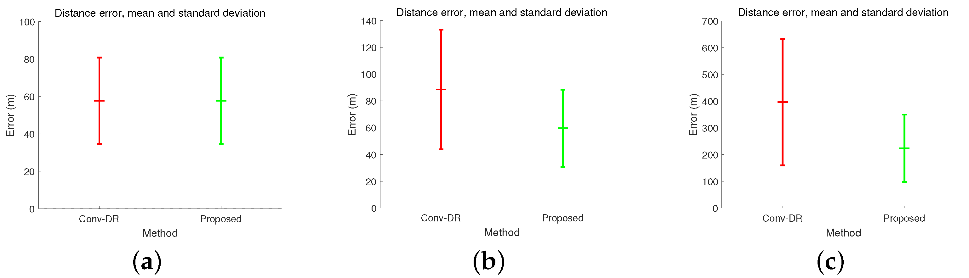
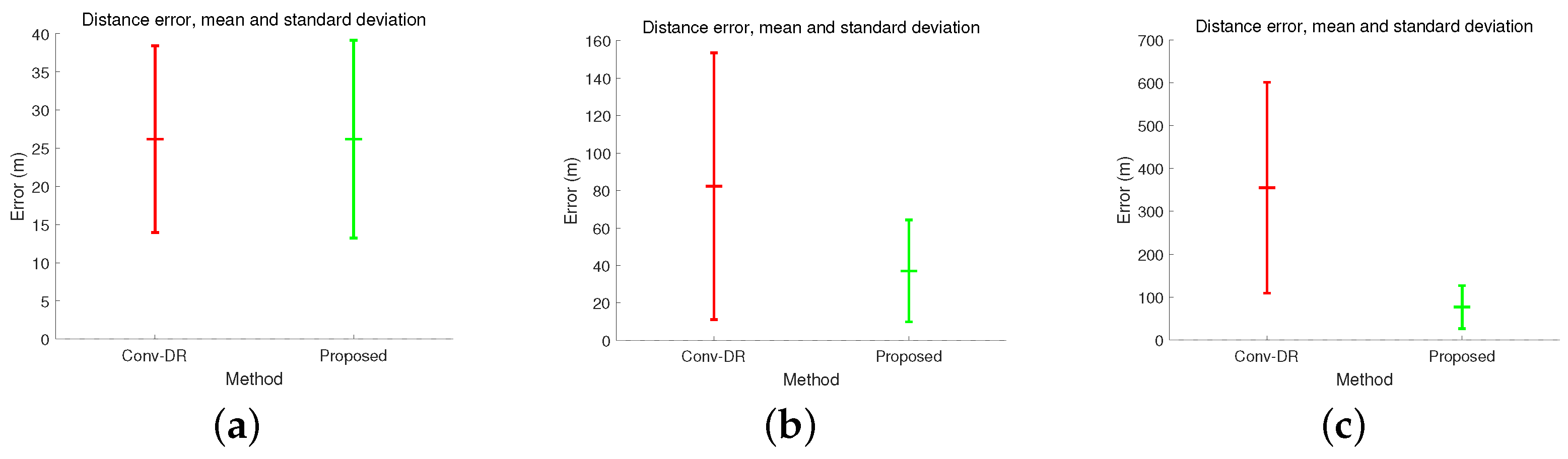
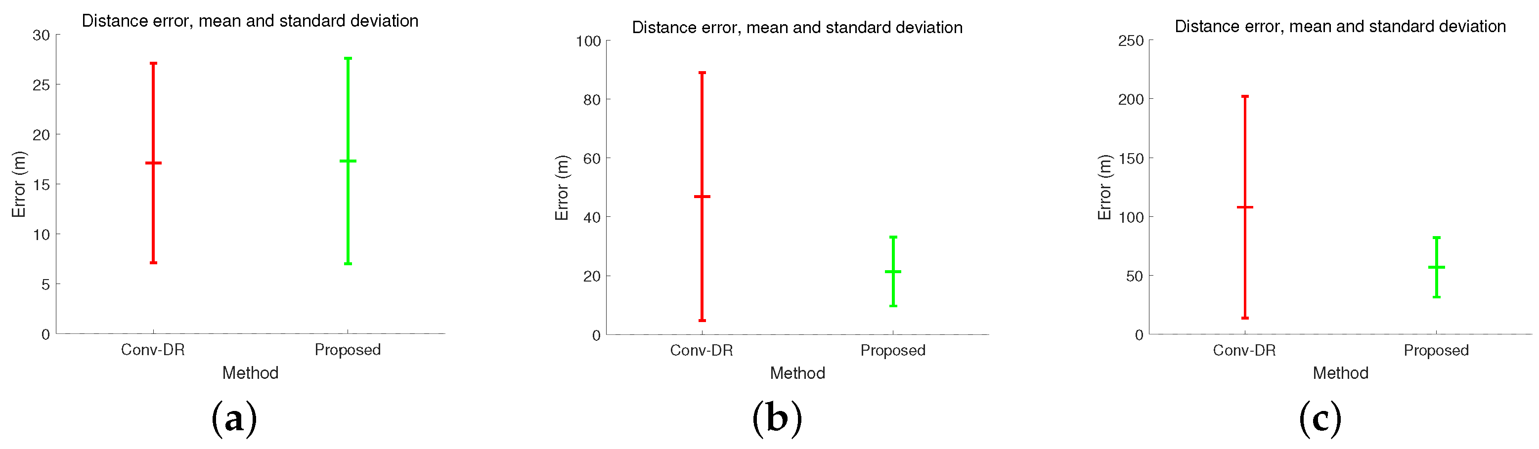
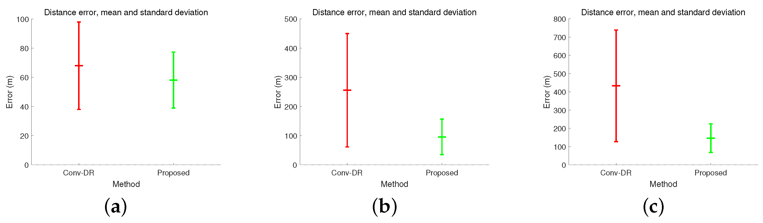
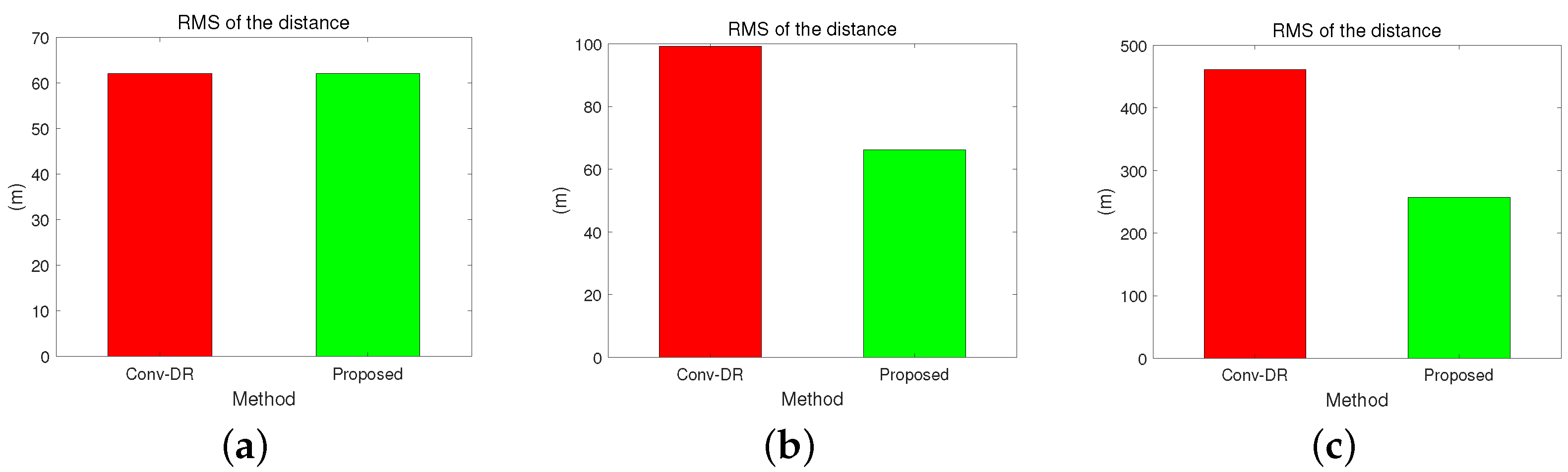
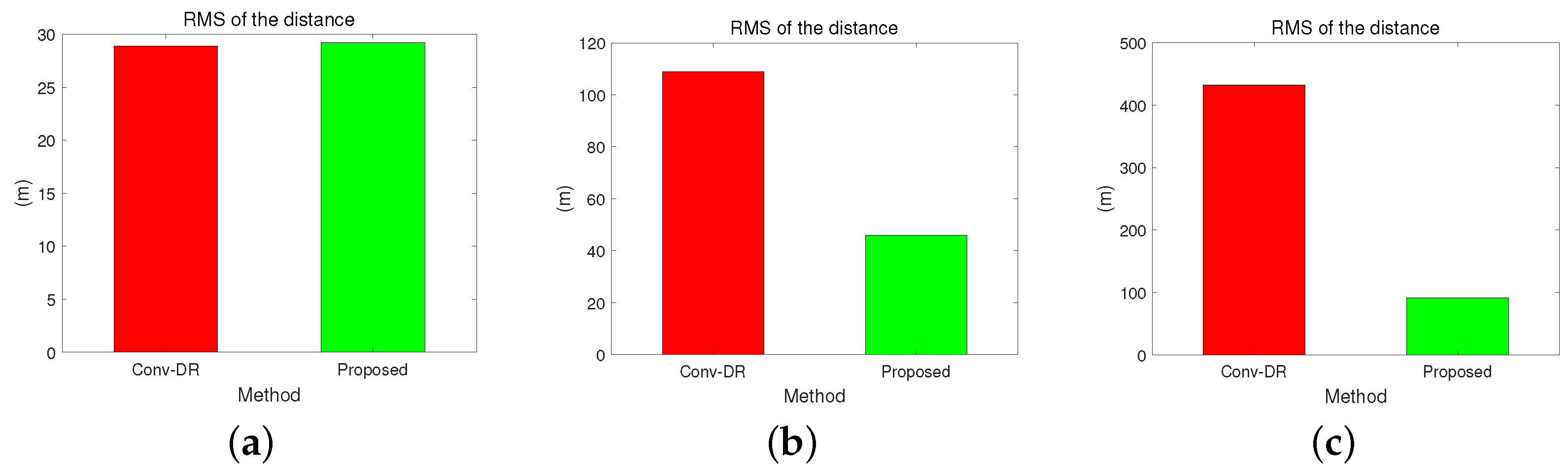
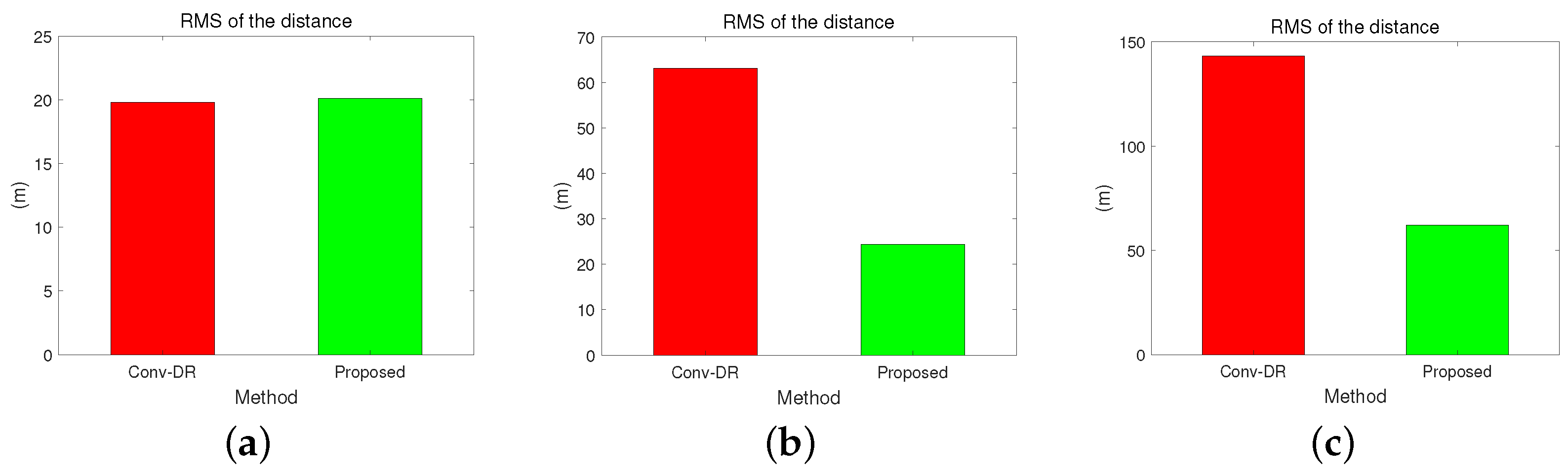
Figure 8, Figure 9, Figure 10, Figure 11, Figure 12, Figure 13, Figure 14 and Figure 15 graphically compare the distance errors of position prediction based on Table 2. The path predicted by the proposed method is closer to the true path than that predicted by the previous method. Any trajectory error in the proposed method arises from errors in measured velocity and inherent computation. Unlike Equations (9), (11) and (12), the motion Equation (16) does not involve any approximation. Additionally, the proposed method can reduce cumulative errors, thereby improving accuracy even when the data reception period is long. These results demonstrate the overall effectiveness of the proposed method under various conditions.

Figure 8.
Comparison of distance error, mean, and standard deviation in region (1): (a) has a data reception period of 0.1 s; (b) has a data reception period of 0.5 s; and (c) has a data reception period of 1 s.

Figure 9.
Comparison of distance error, mean, and standard deviation in region (2): (a) has a data reception period of 0.1 s; (b) has a data reception period of 0.5 s; and (c) has a data reception period of 1 s.

Figure 10.
Comparison of distance error, mean, and standard deviation in region (3): (a) has a data reception period of 0.1 s; (b) has a data reception period of 0.5 s; and (c) has a data reception period of 1 s.
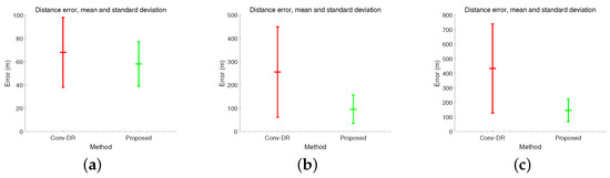
Figure 11.
Comparison of distance error, mean, and standard deviation in region (4): (a) has a data reception period of 0.1 s; (b) has a data reception period of 0.5 s; and (c) has a data reception period of 1 s.

Figure 12.
Comparison of distance error, including RMS, in region (1): (a) has a data reception period of 0.1 s; (b) has a data reception period of 0.5 s; and (c) has a data reception period of 1 s.

Figure 13.
Comparison of distance error, including RMS, in region (2): (a) has a data reception period of 0.1 s; (b) has a data reception period of 0.5 s; and (c) has a data reception period of 1 s.

Figure 14.
Comparison of distance error, including RMS, in region (3): (a) has a data reception period of 0.1 s; (b) has a data reception period of 0.5 s; and (c) has a data reception period of 1 s.
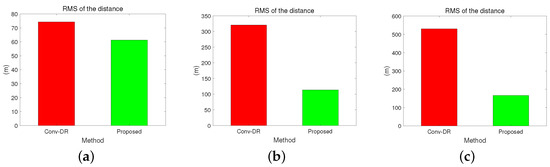
Figure 15.
Comparison of distance error, including RMS, in region (4): (a) has a data reception period of 0.1 s; (b) has a data reception period of 0.5 s; and (c) has a data reception period of 1 s.
4.3. Speed Results
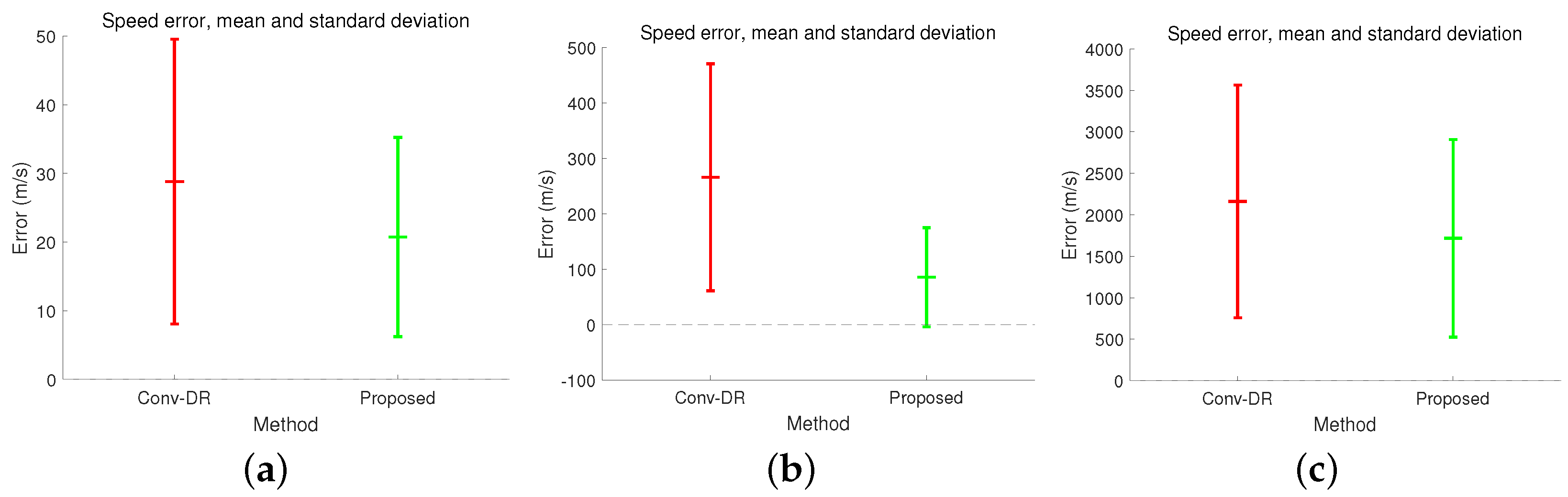
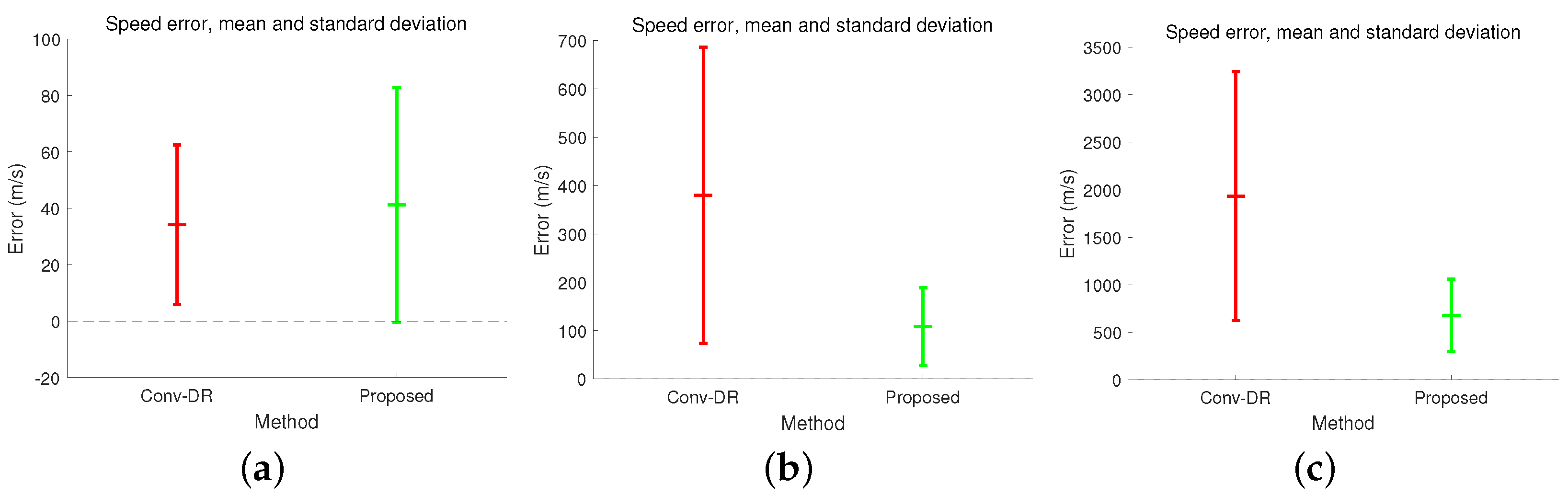
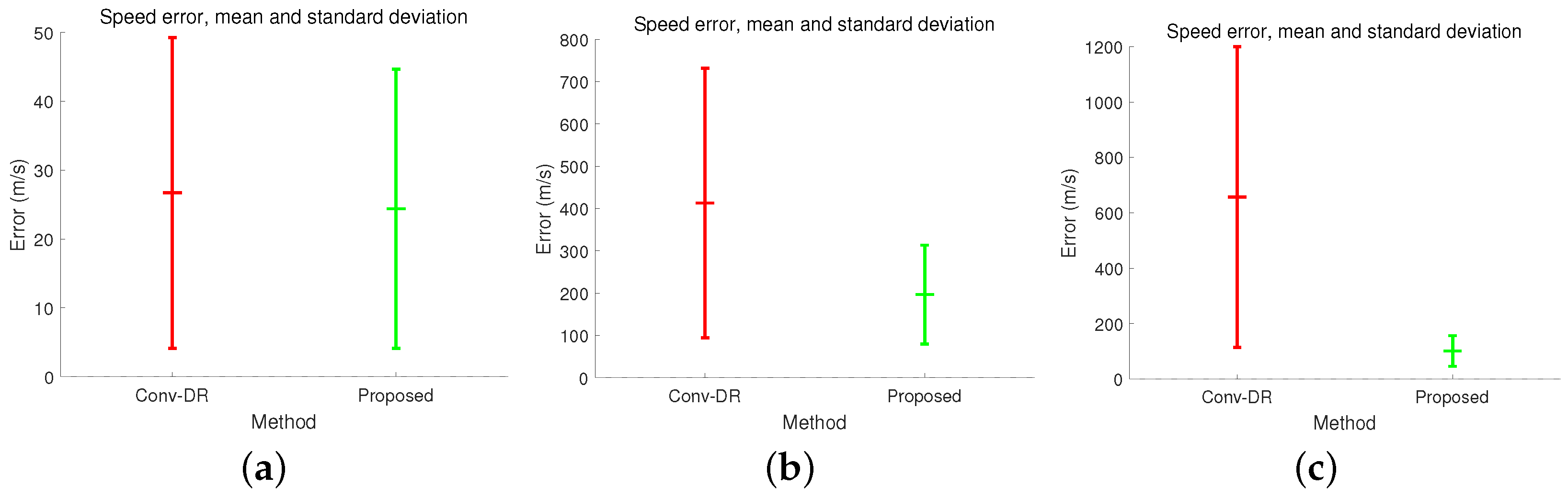
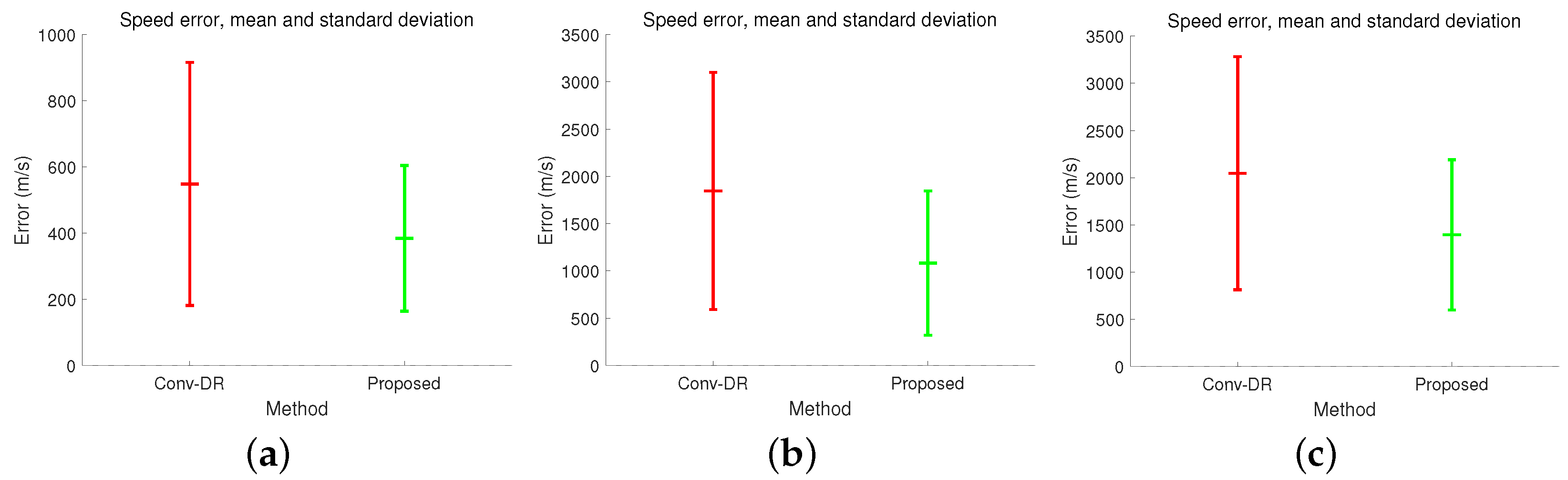
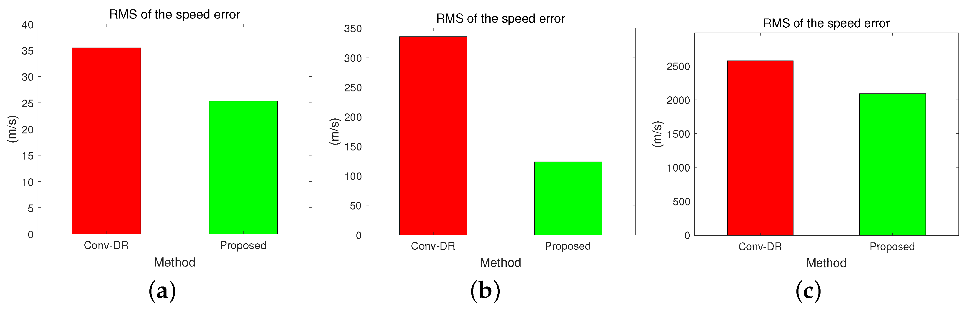
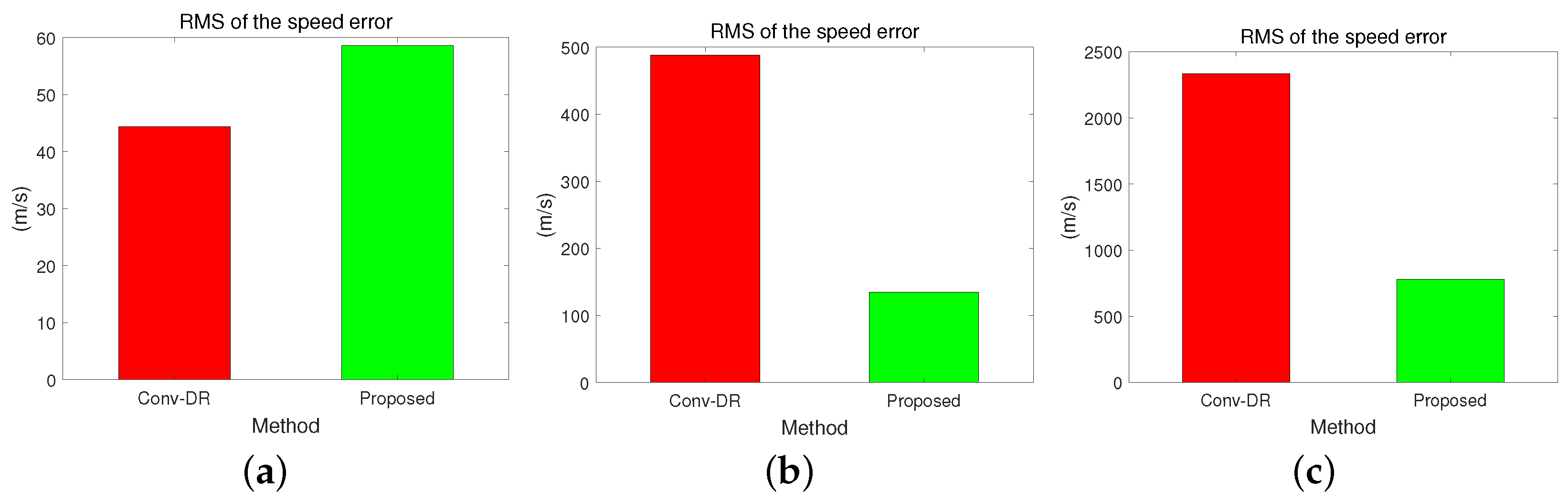
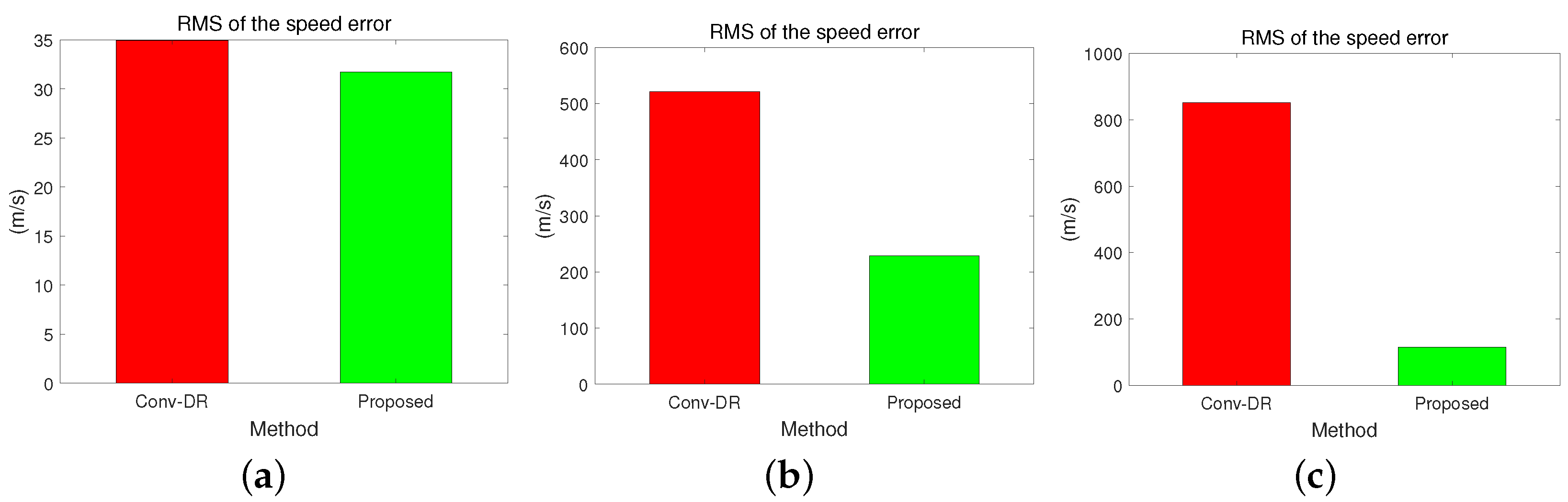
The calculated velocity errors in the ENU coordinate frame were compared with the previously used DR errors. The reference velocity was obtained using the speed output from the GPS. Figure 16, Figure 17, Figure 18, Figure 19, Figure 20, Figure 21, Figure 22 and Figure 23 graphically compare the errors in velocity prediction based on Table 3. Similar to the position results, the proposed method shows mostly smaller or similar results in mean error, standard deviation, and RMS values compared to the previously widely used DR. Additionally, the proposed method shows improved results in terms of velocity prediction accuracy as the data reception cycle becomes longer. Unlike the previously widely used DR, the proposed method performs accurate calculations in nonlinear space. However, the previously widely used DR considers attitude as a variable in linear space. Therefore, the previously widely used DR employs typical arithmetic operations. These operations lead to approximation errors.

Figure 16.
Comparison of speed error, mean, and standard deviation in region (1): (a) has a data reception period of 0.1 s; (b) has a data reception period of 0.5 s; and (c) has a data reception period of 1 s.

Figure 17.
Comparison of speed error, mean, and standard deviation in region (2): (a) has a data reception period of 0.1 s; (b) has a data reception period of 0.5 s; and (c) has a data reception period of 1 s.

Figure 18.
Comparison of speed error, mean, and standard deviation in region (3): (a) has a data reception period of 0.1 s; (b) has a data reception period of 0.5 s; and (c) has a data reception period of 1 s.

Figure 19.
Comparison of speed error, mean, and standard deviation in region (4): (a) has a data reception period of 0.1 s; (b) has a data reception period of 0.5 s; and (c) has a data reception period of 1 s.

Figure 20.
Comparison of speed error, including RMS, in region (1): (a) has a data reception period of 0.1 s; (b) has a data reception period of 0.5 s; and (c) has a data reception period of 1 s.

Figure 21.
Comparison of speed error, including RMS, in region (2): (a) has a data reception period of 0.1 s; (b) has a data reception period of 0.5 s; and (c) has a data reception period of 1 s.

Figure 22.
Comparison of speed error, including RMS, in region (3): (a) has a data reception period of 0.1 s; (b) has a data reception period of 0.5 s; and (c) has a data reception period of 1 s.
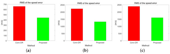
Figure 23.
Comparison of speed error, including RMS, in region (4): (a) has a data reception period of 0.1 s; (b) has a data reception period of 0.5 s; and (c) has a data reception period of 1 s.
Table 3.
Analysis of the speed error in the ENU coordinate frame.
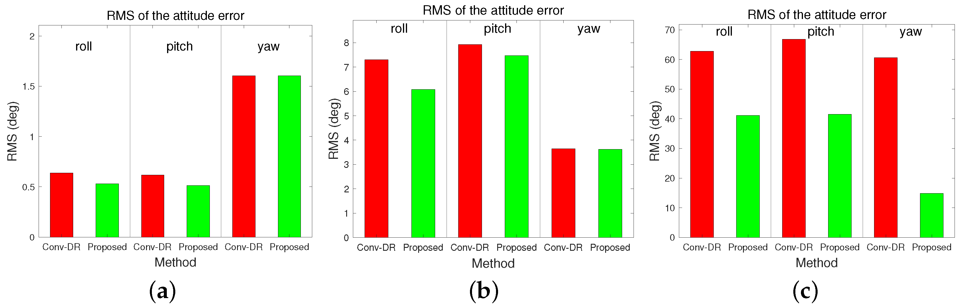
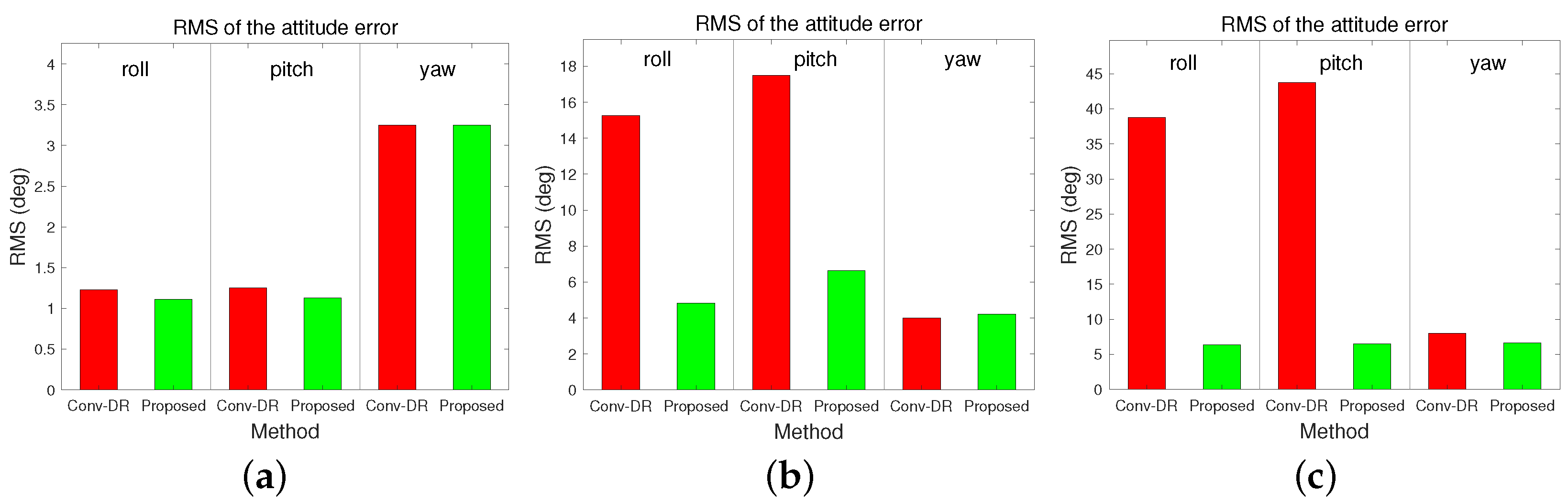
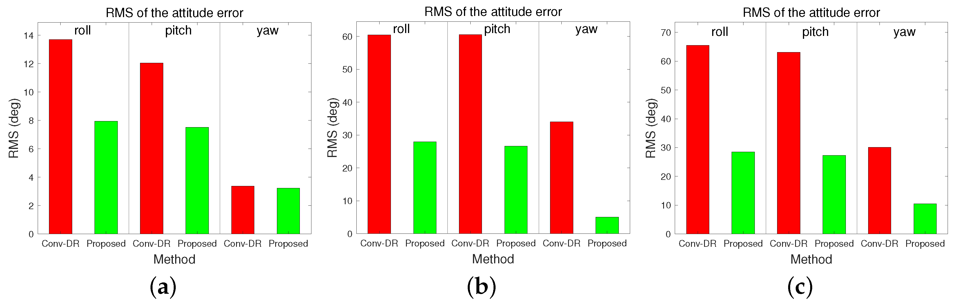
4.4. Attitude Results
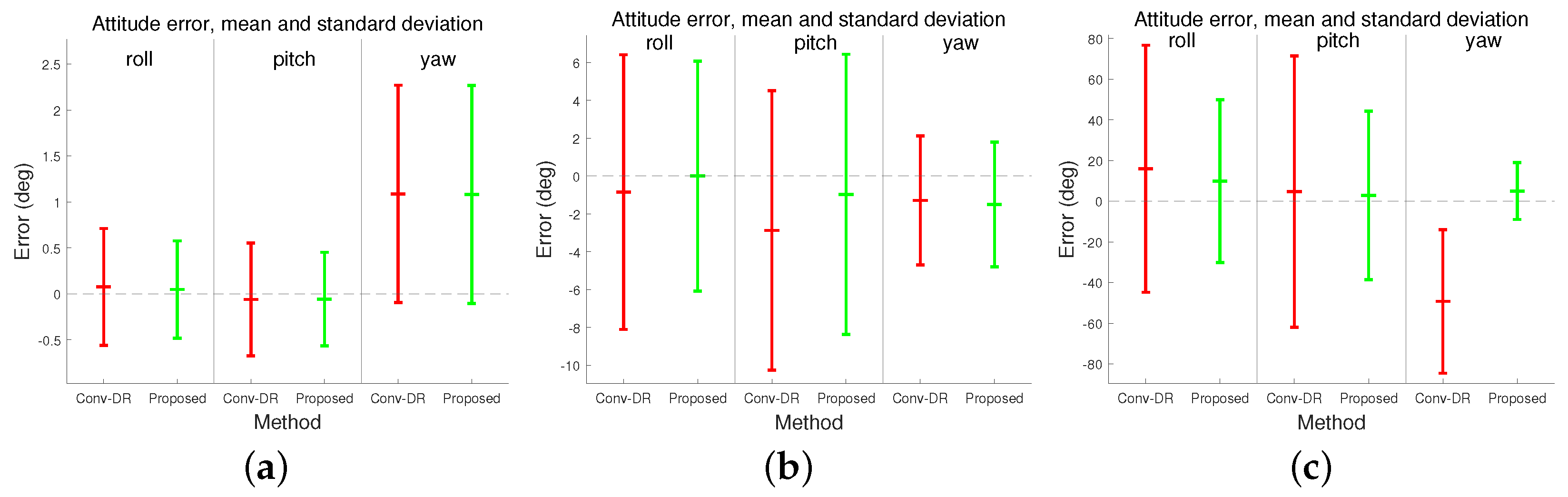
Figure 24, Figure 25, Figure 26, Figure 27, Figure 28, Figure 29, Figure 30 and Figure 31 graphically compare the errors in attitude based on Table 4. It can be confirmed that the proposed method shows mostly smaller values in mean error, standard deviation, and RMS. Attitude and rotation cannot be perfectly represented and computed in linear space. The previously widely used DR inevitably includes errors that occur in the linearization process. However, the proposed method accurately represents attitude and handles operations in a nonlinear space called the Lie group. Therefore, it does not cause errors that force approximation into a linear space, and it was able to reduce the overall DR error.

Figure 24.
Comparison of attitude error, mean, and standard deviation in region (1): (a) has a data reception period of 0.1 s; (b) has a data reception period of 0.5 s; and (c) has a data reception period of 1 s.

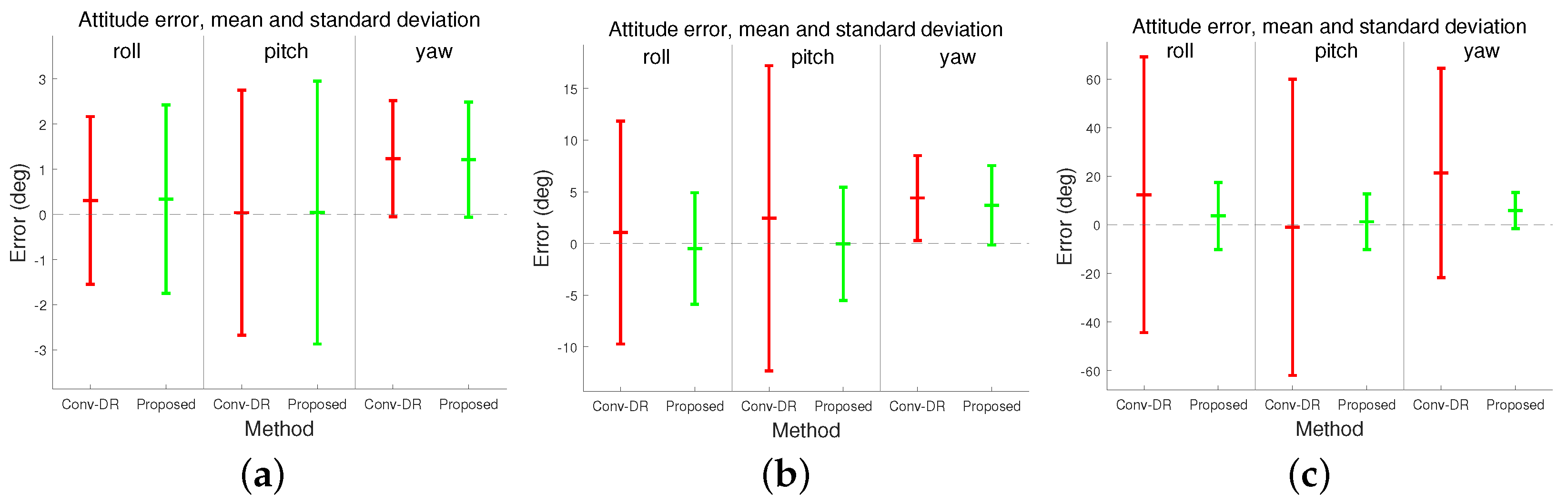
Figure 25.
Comparison of attitude error, mean, and standard deviation in region (2): (a) has a data reception period of 0.1 s; (b) has a data reception period of 0.5 s; and (c) has a data reception period of 1 s.

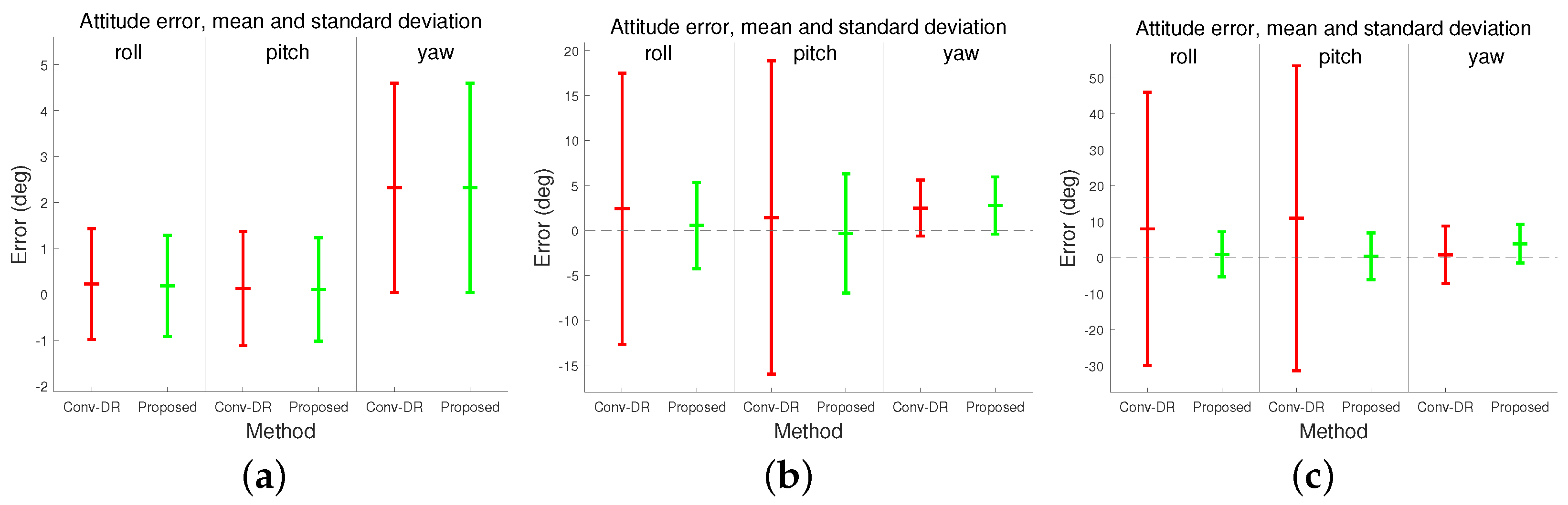
Figure 26.
Comparison of attitude error, mean, and standard deviation in region (3): (a) has a data reception period of 0.1 s; (b) has a data reception period of 0.5 s; and (c) has a data reception period of 1 s.

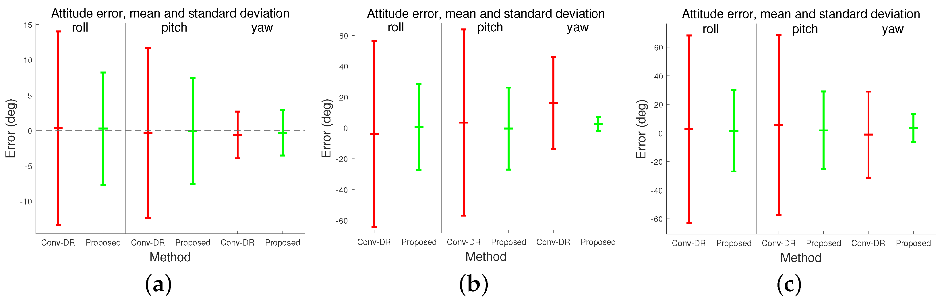
Figure 27.
Comparison of attitude error, mean, and standard deviation in region (4): (a) has a data reception period of 0.1 s; (b) has a data reception period of 0.5 s; and (c) has a data reception period of 1 s.

Figure 28.
Comparison of attitude error, including RMS, in region (1): (a) has a data reception period of 0.1 s; (b) has a data reception period of 0.5 s; and (c) has a data reception period of 1 s.
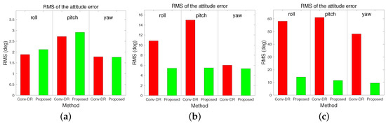
Figure 29.
Comparison of attitude error, including RMS, in region (2): (a) has a data reception period of 0.1 s; (b) has a data reception period of 0.5 s; and (c) has a data reception period of 1 s.

Figure 30.
Comparison of attitude error, including RMS, in region (3): (a) has a data reception period of 0.1 s; (b) has a data reception period of 0.5 s; and (c) has a data reception period of 1 s.

Figure 31.
Comparison of attitude error, including RMS, in region (4): (a) has a data reception period of 0.1 s; (b) has a data reception period of 0.5 s; and (c) has a data reception period of 1 s.
Table 4.
Analysis of the attitude error.
5. Conclusions
This paper presents a novel approach to DR for vehicles. This method utilizes Lie theory by treating the position and velocity of the vehicle as elements of the Lie group . Previously widely used DR methods have faced challenges due to approximation errors when handling nonlinear transformations and uncertainties. However, this method enables accurate solutions without linear approximation errors by treating the position and velocity of the vehicle as elements of a Lie group. In the DR operation process, the increments for pose and velocity are expressed in the Lie algebra, which is a linear space. Real-world experimental results have confirmed that this method improves accuracy. Notably, even when the time interval is long and increments increase, this method significantly reduces errors compared to previously used DR. In other words, the proposed method can overcome approximation errors due to integration and uncertainty errors caused by forced approximation of attitude into a linear space. In future work, the proposed method will be used as a process model in recursive filters such as the KF to improve the accuracy of state prediction. Additionally, the convergence performance of internal parameters such as measurement innovation and Kalman gain will be enhanced based on the improved state prediction values.
Author Contributions
Conceptualization, D.B.J. and N.Y.K.; methodology, D.B.J. and N.Y.K.; software, D.B.J. and N.Y.K.; validation, D.B.J., N.Y.K. and B.L.; formal analysis, D.B.J. and N.Y.K.; investigation, D.B.J., N.Y.K. and B.L.; resources, D.B.J. and N.Y.K.; data curation, D.B.J., N.Y.K. and B.L.; writing—original draft preparation, D.B.J.; writing—review and editing, N.Y.K.; visualization, D.B.J.; supervision, N.Y.K.; project administration, N.Y.K. and B.L.; funding acquisition, N.Y.K. All authors have read and agreed to the published version of the manuscript.
Funding
This research was supported by Basic Science Research Program through the National Research Foundation of Korea (NRF) funded by the Ministry of Education (NRF-2019R1I1A3A01057691).
Institutional Review Board Statement
Not applicable.
Informed Consent Statement
Not applicable.
Data Availability Statement
The original data presented in the study are openly available in [35].
Conflicts of Interest
The authors declare no conflicts of interest.
References
- Hashim, H.A. GPS-denied navigation: Attitude, position, linear velocity, and gravity estimation with nonlinear stochastic observer. In Proceedings of the 2021 American Control Conference, New Orleans, LA, USA, 25–28 May 2021; pp. 1146–1151. [Google Scholar]
- Nezhadshahbodaghi, M.; Mosavi, M.R.; Hajialinajar, M.T. Fusing denoised stereo visual odometry, INS and GPS measurements for autonomous navigation in a tightly coupled approach. GPS Solut. 2021, 25, 47. [Google Scholar] [CrossRef]
- Liao, J.; Li, X.; Wang, X.; Li, S.; Wang, H. Enhancing navigation performance through visual-inertial odometry in GNSS-degraded environment. GPS Solut. 2021, 25, 50. [Google Scholar] [CrossRef]
- Shi, L.F.; Zhao, Y.L.; Liu, G.X.; Chen, S.; Wang, Y.; Shi, Y.F. A robust pedestrian dead reckoning system using low-cost magnetic and inertial sensors. IEEE Trans. Instrum. Meas. 2018, 68, 2996–3003. [Google Scholar] [CrossRef]
- Jeon, J.; Hwang, Y.; Jeong, Y.; Park, S.; Kweon, I.S.; Choi, S.B. Lane detection aided online dead reckoning for GNSS denied environments. Sensors 2021, 21, 6805. [Google Scholar] [CrossRef] [PubMed]
- Nagin, I.A.; Inchagov, Y.M. Effective integration algorithm for pedestrian dead reckoning. In Proceedings of the 2018 Moscow Workshop Electronic and Networking Technologies, Moscow, Russia, 14–16 March 2018; pp. 1–4. [Google Scholar]
- Welte, A.; Xu, P.; Bonnifait, P. Four-wheeled dead-reckoning model calibration using RTS smoothing. In Proceedings of the 2019 International Conference on Robotics and Automation (ICRA), Montreal, QC, Canada, 20–24 May 2019; pp. 312–318. [Google Scholar]
- Zlotnik, D.E.; Forbes, J.R. Exponential convergence of a nonlinear attitude estimator. Automatica 2016, 72, 11–18. [Google Scholar] [CrossRef]
- Hashim, H.A.; Abouheaf, M.; Vamvoudakis, K.G. Neural-adaptive stochastic attitude filter on SO(3). IEEE Control Sys. Lett. 2021, 6, 1549–1554. [Google Scholar] [CrossRef]
- Hashim, H.A. Systematic convergence of nonlinear stochastic estimators on the special orthogonal group SO(3). Int. J. Robust Nonlinear Control 2020, 30, 3848–3870. [Google Scholar] [CrossRef]
- Hashim, H.A.; Brown, L.J.; McIsaac, K. Nonlinear stochastic attitude filters on the special orthogonal group 3: Ito and Stratonovich. IEEE Trans. Sys. Man Cyber. Sys. 2019, 49, 1853–1865. [Google Scholar] [CrossRef]
- Medeiros, R.A.; Pimentel, G.A.; Garibotti, R. Embedded quaternion-based extended Kalman filter pose estimation for six degrees of freedom systems. J. Intell. Robot. Syst. 2021, 102, 18. [Google Scholar] [CrossRef]
- Candan, B.; Soken, H.E. Estimation of attitude using robust adaptive Kalman filter. In Proceedings of the IEEE 8th International Workshop on Metrology for AeroSpace (MetroAeroSpace), Naples, Italy, 23–25 June 2021; pp. 159–163. [Google Scholar]
- Shurin, A.; Klein, I. QuadNet: A Hybrid Framework for Quadrotor Dead Reckoning. Sensors 2022, 22, 1426. [Google Scholar] [CrossRef]
- Jang, E.; Eom, S.-H.; Lee, E.-H. A Study on the UWB-Based Position Estimation Method Using Dead Reckoning Information for Active Driving in a Mapless Environment of Intelligent Wheelchairs. Appl. Sci. 2024, 14, 620. [Google Scholar] [CrossRef]
- Zhang, Y.; Zhang, F.; Wang, Z.; Zhang, X. Localization Uncertainty Estimation for Autonomous Underwater Vehicle Navigation. J. Mar. Sci. Eng. 2023, 11, 1540. [Google Scholar] [CrossRef]
- Bai, L.; Pepper, M.G.; Wang, Z.; Mulvenna, M.D.; Bond, R.R.; Finlay, D.; Zheng, H. Upper Limb Position Tracking with a Single Inertial Sensor Using Dead Reckoning Method with Drift Correction Techniques. Sensors 2023, 23, 360. [Google Scholar] [CrossRef] [PubMed]
- Cao, S.; Jin, Y.; Trautmann, T.; Liu, K. Design and Experiments of Autonomous Path Tracking Based on Dead Reckoning. Appl. Sci. 2023, 13, 317. [Google Scholar] [CrossRef]
- Zhang, L.; Gao, Y.; Guan, L. Optimizing AUV Navigation Using Factor Graphs with Side-Scan Sonar Integration. J. Mar. Sci. Eng. 2024, 12, 313. [Google Scholar] [CrossRef]
- Ma, X.; Liu, X.; Li, C.-L.; Che, S. Multi-source information fusion based on factor graph in autonomous underwater vehicles navigation systems. Assem. Autom. 2021, 41, 536–545. [Google Scholar] [CrossRef]
- Shahoud, A.; Shashev, D.; Shidlovskiy, S. Visual Navigation and Path Tracking Using Street Geometry Information for Image Alignment and Servoing. Drones 2022, 6, 107. [Google Scholar] [CrossRef]
- Yu, Y.; Wang, X.; Shen, L. Optimal UAV Circumnavigation Control with Input Saturation Based on Fisher Information. IFAC-PapersOnLine 2020, 53, 2471–2476. [Google Scholar] [CrossRef]
- Xie, B.; Dai, S. A comparative study of extended Kalman filtering and unscented Kalman filtering on lie group for stewart platform state estimation. In Proceedings of the 2021 6th International Conference on Control and Robotics Engineering (ICCRE), Beijing, China, 16–18 April 2021; pp. 145–150. [Google Scholar]
- Wong, J.N.; Yoon, D.J.; Schoellig, A.P.; Barfoot, T.D. A data-driven motion prior for continuous-time trajectory estimation on SE(3). IEEE Robot. Autom. Lett. 2020, 5, 1429–1436. [Google Scholar] [CrossRef]
- Tang, T.Y.; Yoon, D.J.; Barfoot, T.D. A white-noise-on-jerk motion prior for continuous-time trajectory estimation on SE(3). IEEE Robot. Autom. Lett. 2019, 4, 594–601. [Google Scholar] [CrossRef]
- Luo, Y.; Guo, C.; You, S.; Hu, J.; Liu, J. SE2(3) based Extended Kalman Filter and Smoothing for Inertial-Integrated Navigation. arXiv 2021, arXiv:2102.12897. [Google Scholar]
- Brossard, M.; Barrau, A.; Chauchat, P.; Bonnabel, S. Associating Uncertainty to Extended Poses for on Lie Group IMU Preintegration with Rotating Earth. IEEE Trans. Robot. 2022, 38, 998–1015. [Google Scholar] [CrossRef]
- Hauffe-Waschbüsch, A.; Krieg, A. The Hilbert modular group and orthogonal groups. Res. Number Theory 2022, 8, 47. [Google Scholar] [CrossRef]
- Wu, Y.; Carricato, M. Persistent manifolds of the special Euclidean group SE(3): A review. Comput. Aided Geom. Des. 2020, 79, 101872. [Google Scholar] [CrossRef]
- He, X.; Geng, Z. Trajectory tracking of nonholonomic mobile robots by geometric control on special Euclidean group. Int. J. Robust Nonlinear Control 2021, 31, 5680–5707. [Google Scholar] [CrossRef]
- Jeong, D.B.; Ko, N.Y. Sensor Fusion for Underwater Vehicle Navigation Compensating Misalignment Using Lie Theory. Sensors 2024, 24, 1653. [Google Scholar] [CrossRef] [PubMed]
- Sola, J. Quaternion kinematics for the error-state Kalman filter. arXiv 2017, arXiv:1711.02508. [Google Scholar]
- Sola, J.; Deray, J.; Atchuthan, D. A micro Lie theory for state estimation in robotics. arXiv 2018, arXiv:1812.01537. [Google Scholar]
- Ko, N.Y.; Song, G.; Youn, W.; You, S.H. Lie group approach to dynamic-model-aided navigation of multirotor unmanned aerial vehicles. IEEE Access 2022, 10, 72717–72730. [Google Scholar] [CrossRef]
- Geiger, A.; Lenz, P.; Stiller, C.; Urtasun, R. Vision meets Robotics: The Kitti Dataset. Int. J. Robot. Res. 2013, 32, 1231–1237. [Google Scholar] [CrossRef]


Disclaimer/Publisher’s Note: The statements, opinions and data contained in all publications are solely those of the individual author(s) and contributor(s) and not of MDPI and/or the editor(s). MDPI and/or the editor(s) disclaim responsibility for any injury to people or property resulting from any ideas, methods, instructions or products referred to in the content. |
© 2024 by the authors. Licensee MDPI, Basel, Switzerland. This article is an open access article distributed under the terms and conditions of the Creative Commons Attribution (CC BY) license (https://creativecommons.org/licenses/by/4.0/).