Investigation of Structural Seismic Vulnerability Using Machine Learning on Rapid Visual Screening

Abstract

Seismic vulnerability assessment is one of the most impactful engineering challenges faced by modern societies. Thus, authorities require a reliable tool that has the potential to rank given structures according to their seismic vulnerability. Various countries and organizations over the past decades have developed Rapid Visual Screening (RVS) tools aiming to efficiently estimate vulnerability indices. In general, RVS tools employ a set of structural features and their associated weights to obtain a vulnerability index, which can be used for ranking. In this paper, Machine Learning (ML) models are implemented within this framework. The proposed formulation is used to train binary classifiers in conjunction with ad hoc rules, employing the features of various Codes (e.g., the Federal Emergency Management Agency, New Zealand, and Canada). The efficiency of this modeling effort is evaluated for each Code separately and it is clearly demonstrated that ML-based models are capable of outperforming currently established engineering practices. Furthermore, in the spirit of the aforementioned Codes, a linearization of the fully trained ML model is proposed. ML feature attribution techniques, namely SHapley Additive exPlanations (SHAP) are employed to introduce weights similar to engineering practices. The promising results motivate the potential applicability of this methodology towards the recalibration of the RVS procedures for various types of cases.

1. Introduction

The destructive potential of an earthquake constitutes one of the most severe and impactful engineering challenges faced by modern societies. On the one hand, the global population has increased dramatically during the last century. Coupled with a corresponding increase in urbanization, this has led to a concentration of humans and valuable infrastructure in large urban areas. On the other hand, many structures in the available building stock do not adhere to modern safety standards and, thus, seismic events over the past decades (USA, Turkey, Pakistan, India, Greece, New Zealand) have demonstrated the potential catastrophic results these earthquakes might cause.

Government bodies should be able to identify the most seismically vulnerable buildings in the population. This should enable the allocation of the available resources for preventative actions. In this context, seismic vulnerability refers to the potential of a structure to suffer a certain degree of damage under an earthquake of a predefined intensity level [1,2]. However, the seismic vulnerability of all buildings in a given population cannot be ascertained using the highest possible scrutiny (e.g., using analytical methods like step-by-step dynamic analysis) due to the limitation in resources. To this end, most countries have developed multi-step processes, wherein an initial screening step is performed to identify the potentially most vulnerable structures, which are subjected to further analysis later.

The initial step in the aforementioned processes usually consists of a so-called Rapid Visual Screening (RVS) procedure where structural characteristics that are critical to the overall seismic behavior of the building are rapidly documented by an expert. Such characteristics could include the structural type, the underlying soil, or the height of the building. These are then weighted by expert-defined coefficients to produce a vulnerability index which can be used to rank the given population of structures. The subsequent analysis focuses on the top structures that were obtained according to the respective resource constraints.

The first RVS procedure was developed by the USA Federal Emergency Management Agency (FEMA) in 1988 [3], which was subsequently revised and updated in 2002 [4]. Since the initial version of FEMA 1988, many countries and organizations that face similar challenges have developed their own adaptations of RVS. The most notable ones include the New Zealand Society for Earthquake Engineering [5], the Indian Institute of Technology [6], the Greek Earthquake Planning and Protection Organization (OASP) [7], and the Canadian Office of Critical Infrastructure Protection and Emergency Preparedness (OCIPEP) [8]. Inspired by FEMA, these adaptations share some common elements; however, as their variety indicates, they also have some differences with each other. Indeed, different countries and organizations consider different structural characteristics to be the most crucial and, thus, employ different sets of features in their respective RVS procedures. Even when the same sets of features are employed, different weights can be assigned to them according to the respective experts’ opinions. The accuracy and efficiency of these methodologies can be assessed using data from near-field earthquakes [9,10] which have also been used to calibrate the above procedures [11,12].

On the other hand, the emergence and rapid development of Machine Learning (ML) techniques has highlighted the potential applicability of ML-based methodologies to tackle many complex challenges. To this end, researchers have proposed different approaches that combine the demonstrated power of ML with the established RVS procedures. Yu et al. [13] trained a Convolutional Neural Network (CNN) to ascertain the presence of a soft story, given street view images. Similarly, Ruggieri et al. [14] implemented an ML-based image recognition system to identify the structural parameters of buildings from images which were then employed within the RVS framework to compute a vulnerability score. Bektaş and Kegyes-Brassai [15] employed a Multi-Layer Perceptron (MLP) to predict the damage degree. This was achieved by developing respective classification models using data from the 2015 Nepal earthquake with the corresponding set of features. Finally, Harirchian et al. [16] used data based on RVS features from earthquakes in Ecuador, Haiti, Nepal, and South Korea to assess the predictive power of different ML algorithms, including Support Vector Machines (SVMs), k-Nearest Neighbors (k-NN) and Random Forests.

Novelty of the Research

The novelty and contributions of the present research are twofold. On the one hand, we implement Machine Learning classification models for seismic vulnerability ranking. As a matter of fact, these models perform pairwise comparisons between distinct structures. This methodology is applied to a variety of the most well-known and widely applicable RVS procedures (FEMA, Canada, India, New Zealand, Greece-OASP), to demonstrate its strong potential to outperform the currently established engineering practices. On the other hand, inspired by the linear approaches employed by the existing Codes for the computation of the respective RVS scores, this paper introduces a linearization of the fully trained ML models. Machine learning feature attribution methods are employed to compute the weights for each structural parameter. This procedure aims to provide a technique which can be used to recalibrate the existing methodologies.

The case study of this research is based on real measurements, performed on 457 reinforced concrete structures after the 1999 Athens earthquake. Given the promising results presented herein, the proposed methodologies could be implemented using datasets from different countries and organizations and even different structural types. Even though the features could be different, the data could be used to train the ML models and to obtain recalibrated weights that are more closely attuned to the individual conditions of each Seismic Code.

2. Materials and Methods

2.1. Dataset Description

The dataset employed in the present work consists of a collection of Rapid Visual Screening measurements pertaining to 457 structures. These were drawn after the 7 September 1999 Athens earthquake [17]. The samples in the dataset exhibited a varying degree of damage across the spectrum, ranging from partial or total collapse to moderate or minimal damages. To enhance the dataset diversity, the structures were drawn from various regions in the greater Athens Metropolitan area. This mitigated the influence of local effects, such as distance from the earthquake epicenter or ground conditions, on the observed damage states. The authors in [17] took further steps to mitigate these effects; when one structure was selected from a specific building block, structures across the damage spectrum were also selected from the same area [18]. The observed damage states were classified into four distinct classes, namely:

• “Black”: The category suffering the most severe damages. Structures belonging to this label suffered partial or total collapse during the earthquake, crossing the so-called Collapse Limit State (CLS).
• “Red”: While the structures belonging to this label did not cross the CLS, they suffered extensive damages to their structural members and crossed the so-called Ultimate Limit State (ULS).
• “Yellow”: Structures of this category suffered only moderate damages to their structural members. While these structures did not cross the ULS, they did cross the so-called Serviceability Limit State (SLS).
• “Green”: The structures of this class suffered only minor damages.

The distribution of structures across the damage spectrum is shown in the following

Table 1. Distribution of structures across the damage spectrum.

Damage Label	Number of Structures
Black	93
Red	201
Yellow	69
Green	94

.

Table 2. Attributes employed by each Seismic Code.

Attribute	Seismic Code
	FEMA 1988	FEMA 2002	OASP (2000–2004)	India	Canada	New Zealand
Structural type	✓	✓	✓	✓	✓	✓
Significant height	✓	✓	✓	✓	✗	✓
Poor condition	✓	✗	✓	✗	✓	✗
Vertical irregularity	✓	✓	✓	✓	✓	✓
Horizontal irregularity	✓	✓	✓	✓	✓	✓
Soft story	✓	✓	✓	✓	✓	✓
Torsion	✓	✗	✓	✗	✓	✓
Pounding	✓	✗	✓	✗	✓	✓
Heavy non-structural elements	✓	✗	✓	✗	✗	✓
Short columns	✓	✗	✓	✗	✓	✓
Benchmark year	✓	✓	✓	✓	✓	✓
Soil type	✓	✓	✓	✓	✓	✓
Moderate height	✗	✓	✗	✓	✗	✗
Lack of Seismic Code design	✗	✓	✓	✗	✗	✗
Wall filling regularity	✗	✗	✓	✗	✗	✗
Previous damages	✗	✗	✓	✗	✓	✗

shows which attributes have been considered by each Seismic Code. It is a fact that each code considers its own vector of structural aspects [3,4,5,6,7,8,17].

• Structural type: In general, Seismic Codes distinguish buildings according to their structural type, e.g., framed structures or frames with shear walls [8].
• Significant height: This is an attribute that most Seismic Codes take into consideration. It affects structures whose height exceeds a predefined threshold. However, this threshold varies between Seismic Codes. For example, FEMA sets this threshold at 7 stories, while this threshold for OASP equals 5. In addition to the above, some Seismic Codes, e.g., that of India, distinguish structures with “moderate height” as a separate category.
• Poor condition: This attribute accounts for potential deterioration in the design seismic capacity of the building. This may be due to corroded reinforcement bars or due to poor concrete quality (e.g., aggregate segregation or erosion) [8].
• Vertical irregularity: This attribute pertains to structures with significant variations in their height, which leads to discontinuities in the paths of the vertical loads.
• Horizontal irregularity: This feature affects structures whose floor plans exhibit sharp, re-entrant corners, such as “L”, “T”, or “E”, which have the potential to develop higher degrees of damage [8].
• Soft story: This pertains to structures wherein one story has significantly less stiffness than the rest; for example, due to a discontinuity of the shear walls.
• Torsion: Structures with high eccentricities suffer from torsional loads during an earthquake. This could lead to higher degrees of damage.
• Pounding: This attribute is considered when two adjacent structures do not have a sufficient gap between them and especially when the buildings have different heights, which may lead to the slabs of one structure ramming into the columns of the other.
• Heavy non-structural elements: While they are non-structural, the displacement of such elements during an earthquake can lead to eccentricities and to additional torsion.
• Short columns: This attribute refers to columns wherein modifications have resulted in a reduction in their active length. Such modifications include the addition of spandrel beams, or wall sections that do not cover the full height of the story [8].
• Benchmark year: Various Seismic Codes define the so-called “benchmark years” where an improved version of the Code took effect.
• Soil type: Generally, Seismic Codes classify soil types ranging from rock and semi-rock formations to loose fine-grained silt [19]. The quality of the underlying soil is a significant factor of the overall seismic behavior of the building.
• Lack of Seismic Code design: This attribute pertains to structures that were designed without adhering to the provisions of a dedicated Seismic Code.
• Wall filling regularity: When the infill walls are of sufficient thickness and with few openings, they can support the surrounding frames during an earthquake, leading to improved overall performance.
• Previous damages: This attribute pertains to structures whose previous damages have not been adequately repaired, leading to a deterioration of their overall seismic capacity.

As it is evident from the above, the existing Seismic Codes consider distinct feature vectors in their respective RVS procedures. The selection of these features is based on experts’ knowledge, which varies from country to country and from institution to institution. Even when the same features are used, different weights might be assigned to them and the calculation of the final vulnerability score might be carried out using different procedures. This calls for the need for the use of Machine Learning data-driven models. These models can learn from the spectrum of the available data vectors, and they can lead to ranking improvements, which is the aim of this study.

2.2. Overview of the Proposed Formulation

At high levels, the employed formulation is based on the development of a binary classification model $f:{\mathbb{R}}^n\times {\mathbb{R}}^n\to \{-1,+1\}$ that can effectively consider a pair of feature vectors ${\mathbf{x}}_i,{\mathbf{x}}_j\in {\mathbb{R}}^n$, corresponding to a respective pair of structures $s_i,s_j$ in order to rank them. More specifically, the formulation predicts whether $s_j$ should rank higher than $s_j$ (“+1”) or vice versa (“−1”). Overall, the algorithm proceeds as shown in Algorithm 1 and Figure 1 presented below [20]:

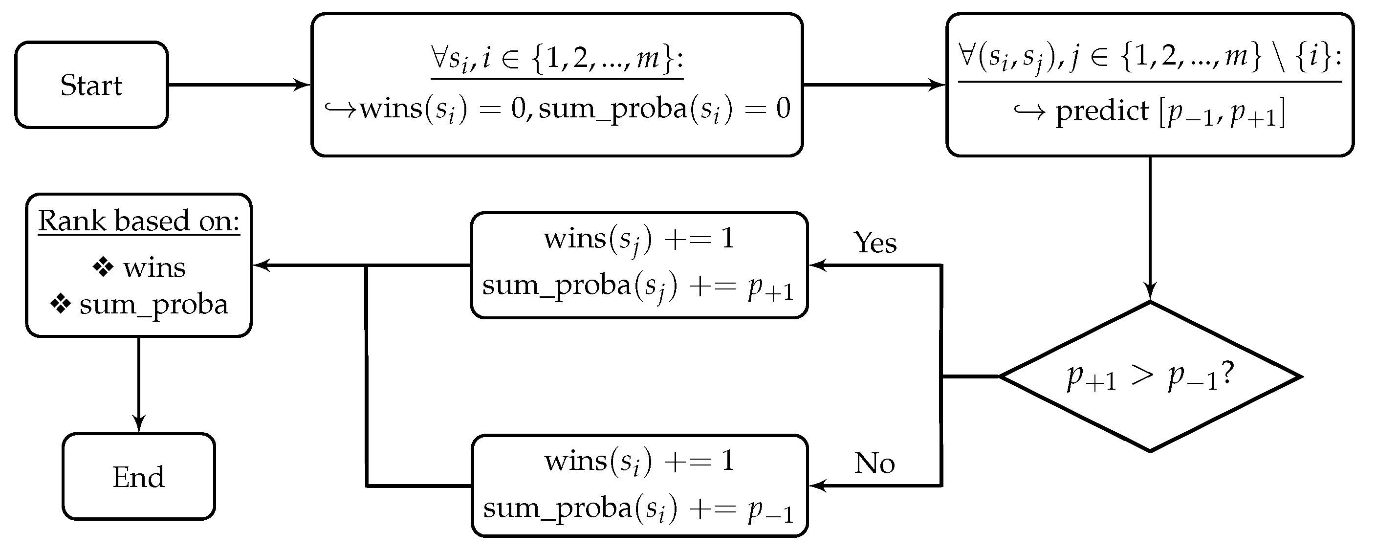
Algorithm 1 Algorithmic seismic vulnerability ranking process using ML model [20].

for $i=1,2,\dots ,m$ do:    Initialize $\mathrm{wins}\left(s_i\right)=0,\mathrm{sum}\text{\_}\mathrm{proba}\left(s_i\right)=0$    for $j=1,2,\dots ,m,j\ne i$ do:          Compute ${\mathbf{x}}_{\mathrm{new}}$ and predict the class probabilities $\left[p_{-1},p_{+1}\right]$          if $p_{+1}>p_{-1}$:             $\mathrm{wins}\left(s_j\right)=0 +=1$, $\mathrm{sum}\text{\_}\mathrm{proba}\left(s_j\right)+=p_{+1}$          else:             $\mathrm{wins}\left(s_i\right)=0 +=1$, $\mathrm{sum}\text{\_}\mathrm{proba}\left(s_i\right)+=p_{-1}$    end for end for Rank the given population of structures based on the total number of “wins”, using the running sum of probabilities as a secondary metric.

Using the above algorithm, originally introduced in [20], the problem of seismic vulnerability ranking can be effectively reduced to that of binary classification.

2.3. Data Preprocessing

Data preprocessing is a vital step in a ML model, which not only prepares the dataset in a form that can be considered by the ML models, but it can also directly affect their performance. The following steps were undertaken in this study.

First, as can be seen in Table 1, the “Red” class heavily dominates the dataset. This leads to the well-known “class imbalance problem”. This problem significantly deteriorates the performance of any ML modeling effort. The developed model is always skewed towards the majority class and it cannot effectively adapt to the feature values related to the minority class. This leads to biased models models which lose the ability to generalize [21,22]. To this end, we undersampled the majority class by a factor of 50% to produce a more balanced dataset [23,24].

Subsequently, the features were transformed using numerical values. Indeed, most of the features in Table 2 are binary, indicating whether the structure had the specific attribute. We modeled these features using the 0, 1 values. Similarly, features like soil or structural type, which had distinct values, were modeled using integers. The damage grades were also modeled with integer values, i.e., {Green, Yellow, Red, Black} → {1, 2, 3, 4} [18,20].

Finally, as shown in the previous section, the ML models were trained to receive a pair of structures $s_i,s_j$ with the corresponding feature vectors ${\mathbf{x}}_i,{\mathbf{x}}_j$ as the input and to predict either “−1” or “+1” as the output, i.e., which of the two given structures should rank higher. To achieve this, the pairwise transformation $T:{\mathbb{R}}^n\times {\mathbb{R}}^n\to {\mathbb{R}}^n$ given by $T\left({\mathbf{x}}_i,{\mathbf{x}}_j\right)={\mathbf{x}}_j-{\mathbf{x}}_i$ was employed [20].This resulted in a transformed input dataset, ${\mathbf{X}}^{new}$, with rows corresponding to the pairwise transformed vectors $T\left({\mathbf{x}}_i,{\mathbf{x}}_j\right)$. It should be noted that for each individual seismic Code, the corresponding vectors ${\mathbf{x}}_i$ contain only the features that the respective Code utilizes, as shown in Table 2. Similarly, a transformed output variable $y^{new}$ was obtained. For a pair of structures $s_i,s_j$ with the original target variables $y_i,y_j,y_i\ne y_j$, the corresponding entry in $y^{new}$ is defined as $sign(y_j-y_i)$, where $sign$ denotes the sign() function. Thus, ${\mathbf{X}}^{new}$ and $y^{new}$ were the input and output variables of the trained ML models.

2.4. Machine Learning Algorithm

As has already been mentioned in Section 2.2, using the proposed formulation, the problem of seismic vulnerability ranking was converted to a binary classification problem. There are many available algorithms in the literature for this task [25,26]. Working on the same dataset as OASP (Greece), the authors in [18,20] have compared a variety of different ML models and they have concluded that the Gradient Boosting (GB) classifier offers the highest performance. Extending the previously established results, we will also employ GB in the sequel and to this end we are presenting a short overview of the algorithm.

Gradient Boosting [27] belongs to the group of the ensemble classifiers [28]. It combines a large number of individual “weak” learners, most often Decision Trees [29]. Specifically, the algorithm incrementally learns a function with the form

$$f\left(\mathbf{x}\right)=\sum _{i=1}^N{\alpha }_i{h}_i(\mathbf{x};{\theta }_i).$$

(1)

The $h_i(\mathbf{x};{\theta }_i)$ stands for the “weak” learners whose parameters ${\theta }_i$ are trained during the iterations, N is a hyperparameter denoting the maximum number of such models and $a_i$ is the learned weights of the ensemble. These are learned via a process known as “boosting” [30], wherein the model iteratively computes the gradient of an arbitrary differentiable loss function $\mathcal{L}$ which is used as an input to train the next iteration. An overview of the process is shown in the following Algorithm 2 [27]. The algorithm was implemented using the Python programming language (v. 3.11.5) and the dedicated Machine Learning library scikit-learn (v. 1.3.0) [31].

Algorithm 2 Gradient Boosting learning process [27].

Initialize $F_0\left(\mathbf{x}\right)$ for $i=1,2,\dots ,N$ do:    Compute $w_j\left({\mathbf{x}}_j\right)={\left.\frac{\partial \mathcal{L}(y_j,F\left({\mathbf{x}}_j\right))}{\partial F\left({\mathbf{x}}_j\right)}\right|}_{F\left(\mathbf{x}\right)=F_{i-1}\left(\mathbf{x}\right)},j=1,2,\dots M$    Compute ${\theta }_i=\underset{\theta ,\mu }{argmin}{\displaystyle \sum _{j=1}^M}{\left[-w_j\left({\mathbf{x}}_j\right)-\mu h_i(\mathbf{x};{\theta }_i)\right]}^2$    Compute ${\alpha }_i=\underset{\alpha }{argmin}{\displaystyle \sum _{j=1}^M}\mathcal{L}(y_j,f_{i-1}+\alpha h_i(\mathbf{x};{\theta }_i))$    Update $f_i\left(\mathbf{x}\right)=f_{i-1}\left(\mathbf{x}\right)+\lambda {\alpha }_i{h}_i(\mathbf{x};{\theta }_i))$ end for

2.5. Proposed Methodology for the Recalibration of RVS Using Machine Learning

As we will examine in the next paragraphs, a hybrid approach that employs the algorithm presented in Section 2.2, in conjunction with the Gradient Boosting classifier presented in Section 2.4, can significantly improve the performance of the currently established RVS procedures for the examined Seismic Codes. In this Section, we examine the potential extension of the above methodology towards a closer alignment with the spirit of the aforementioned Codes. Our motivation stems from the fact that, as is well known, most of the Seismic Codes examined herein and presented in Table 2 are additive. Specifically, each of the features they utilize is assigned a weight, $\Delta V_m$, which can be either negative or positive, and the final vulnerability index is obtained as

$$V_I=V_I^b+\sum \Delta V_m,$$

(2)

wherein $V_I^b$ is a basic vulnerability index which varies in different Seismic Codes. The structures in the population can then be ranked in ascending order of the above computed index. One notable exception is the Canadian Code. In this RVS approach, the employed features are first grouped into intermediate variables pertaining to seismicity, soil conditions structural type, and any potential irregularities. These intermediate variables are obtained in an additive way, while the final index is the product of the intermediate variables. Furthermore, the final ranking is obtained in descending order of the index, unlike most other Codes.

The above observations, especially in the form of (2), provide the motivation for a potential recalibration of RVS using the examined novel pairwise formulation. Indeed, for each Seismic Code, we can define a weight vector $\mathbf{w}=\{w_1,w_2,\dots ,w_n\}$, where n is the number of features of each Seismic Code. Thus, these weights are completely analogous to $\Delta V_m$. Furthermore, these weights allow us to modify Algorithm 1 presented in Section 2.2 as shown in Algorithm 3.

Algorithm 3 Algorithmic seismic vulnerability ranking process using the proposed recalibration procedure.

for $i=1,2,\dots ,m$ do:    Initialize $\mathrm{wins}\left(s_i\right)=0,\theta \left(s_i\right)=0$    for $j=1,2,\dots ,m,j\ne i$ do:          Compute ${\mathbf{x}}_{\mathrm{new}}$ and compute $\theta =\mathbf{w}·({\mathbf{x}}_j-{\mathbf{x}}_i)$          if $\theta >0$:                   $\mathrm{wins}\left(s_j\right)=0 +=1$, $\theta \left(s_j\right)+=\theta$          else:                   $\mathrm{wins}\left(s_i\right)=0 +=1$, $\theta \left(s_i\right)+=\theta$    end for end for Rank the given population of structures based on the total number of “wins”, using the running sum $\theta$ as a secondary metric.

This procedure is fundamentally different from the way RVS rankings are obtained in the established literature. However, it is not independent from the Machine Learning methodology examined in Section 2.2, since, as we will analyze, these weights are obtained from the fully trained ML models using the so-called SHapley Additive exPlanations (SHAP) values. It should be reiterated that the aim of this study is not to provide the values of the weights themselves, but rather to demonstrate a procedure for their estimation. Given the promising results presented in the present study, it is hoped that the proposed methodology will be applied to larger datasets, specifically tailored to each country’s seismic demands, which will yield a more accurate calibration of the models for each individual Seismic Code.

2.6. Explainability and SHAP Values

SHapley Additive exPlanations (SHAP) is a feature attribution methodology recently introduced by Lundberg and Lee [32]. They are based on the so-called Shapley values proposed by Lloyd Shapley in the field of cooperative game theory [33]. They are used to analyze the predictions of a trained Machine Learning model into components pertaining to each individual feature. Specifically, given a trained model f, a local approximation h is constructed as follows [32]:

$$h\left(\mathbf{z}\right)={\varphi }_0+\sum _{i=1}^m{\varphi }_i{z}_i,$$

(3)

where m is the number of features employed by the machine learning model, $\mathbf{z}\in {\{0,1\}}^m$ is a binary vector indicating whether the $i^{\mathrm{th}}$ feature was used in the prediction, and ${\varphi }_i$ is the SHAP values corresponding to that feature. The values of ${\varphi }_i$ are computed in such a way that the so-called “local accuracy” property holds [32], i.e., that they approximate the behavior of the underlying model f. To this end, they are given by the formula [32,34]

$${\varphi }_i=\sum _{S\subseteq N\backslash \left\{i\right\}}\frac{\left|S\right|!(n-|S|-1)!}{n!}\left[f(S\cup \{i\left\}\right)-f\left(S\right)\right].$$

(4)

Following the notation of Lundberg et al., in the above Equation (4) $M=1,2,\dots ,m$ is the set of features employed by f and $S\subset M$ is a subset of M called “coalition”, using the term from cooperative game theory. Intuitively, the contribution of each feature is measured as a weighted average of the model’s predictions with and without the inclusion of the particular feature.

The above provides a motivation to employ these SHAP values as the weights $\mathbf{w}$ in our proposed formulation for the recalibration of RVS, which was presented in Section 2.5. However, these SHAP values are computed for each individual data point in the dataset, i.e., for each individual pair of structures. Thus, they are given in the form of a matrix ${\mathbf{\Phi }}^{k\times m}$, where k is the number of pairs of structures in the transformed dataset and m is the number of features each Seismic Code employs. In order to provide a single weight for the whole dataset, the computed values must be aggregated. To this end, we employed a normalized (dividing by the dimension of the vector) norm of each column in the matrix. The ${\mathcal{L}}_1$ norm, i.e., the sum of absolute squares, is one of the most commonly employed ones in the literature. As an alternative, we employed the ${\mathcal{L}}_2$ norm, i.e., the well-known Euclidean norm. Specifically, we computed [18]

$${\overline{\varphi }}_j=\left\{\begin{array}{cc}{\displaystyle \frac{1}{m}\sum _{i=1}^m\left|{\varphi }_{ij}\right|,}\hfill & \mathrm{using}{\mathcal{L}}_1\hfill \\ {\displaystyle \frac{1}{m}\sqrt{{\displaystyle \sum _{i=1}^m}{\varphi }_{ij}^2},}\hfill & \mathrm{using}{\mathcal{L}}_2\hfill \end{array}\right..$$

(5)

A fundamental difference between the two is that the ${\mathcal{L}}_2$ norm tends to reduce the contribution of small, noisy components, while simultaneously highlighting the effect of the most prominent features [18]. This is due to the fact that it is based on squaring the terms before summation. Thus, using the ${\overline{\varphi }}_j$ as defined in (5), we can define the weights $\mathbf{w}$ of our proposed recalibration procedure for RVS. In the present study, the formulations using ${\mathcal{L}}_2$ outperformed the formulation using ${\mathcal{L}}_1$. Thus, the results we will present are based on this approach. The computation of the SHAP values was carried out using the dedicated Python library by Lundberg et al. [35].

3. Results

In this section, we present the results of the present study. As was mentioned in the Introduction, the goal of this study is twofold: on the one hand, it aims to demonstrate that the proposed formulation, as presented in Section 2.2, outperforms the currently established engineering practices in terms of the seismic vulnerability ranking for all the studied Seismic Codes, some of which are the most applicable at an international level. On the other hand, it aims to employ the fully trained Machine Learning models in order to propose a potential recalibration procedure of the aforementioned Codes.

In order to measure the efficiency of the ranking, we compare it with the “ideal” ranking, i.e., how a human would rank the given structures, having perfect knowledge of their damage labels. Indeed, according to this “ideal” ranking, the first 93 structures should be the ones that suffered total or partial collapse (Black), the following 100 structures (post undersampling) should be the ones that were severely damaged, but did not cross the CLS (Red) and so on. Using the above, the predicted ranking can be subdivided into bins, where each bin’s size is the number of structures of the corresponding damage label. In addition, given a damage index {Black, Red, Yellow, Green}, let $bi{n}_d^{true},bi{n}_d^{pred}$ denote the structures that belong to this label and the structures that the algorithm ranked in the corresponding bin, respectively. The efficiency of the ranking was measured using the bin accuracy (BAC) defined as [20]

$${\mathrm{BAC}}_d=\frac{|bi{n}_d^{true}\cap bi{n}_d^{pred}|}{|bi{n}_d^{true}|}.$$

(6)

Other alternative metrics have also been proposed in the literature. For example, in [36], the authors performed a linear regression to obtain a correlation metric between the observed damage labels and the computed RVS score. However, in the present study, we obtained the ranking directly, without computing a similar score beforehand.

Using the metric defined in (6), we computed the bin accuracy for all damage labels and for each individual Seismic Code. First, we computed the accuracy that was obtained using the RVS scores as given by the Codes in their current form. Subsequently, we obtained the accuracy using the fully trained Machine Learning model. Finally, we computed the accuracy obtained using the ML-based recalibrated RVS procedure, as described in Section 2.5 and Section 2.6. The results are shown in

Table 3. Bin accuracy obtained using the established RVS scores.

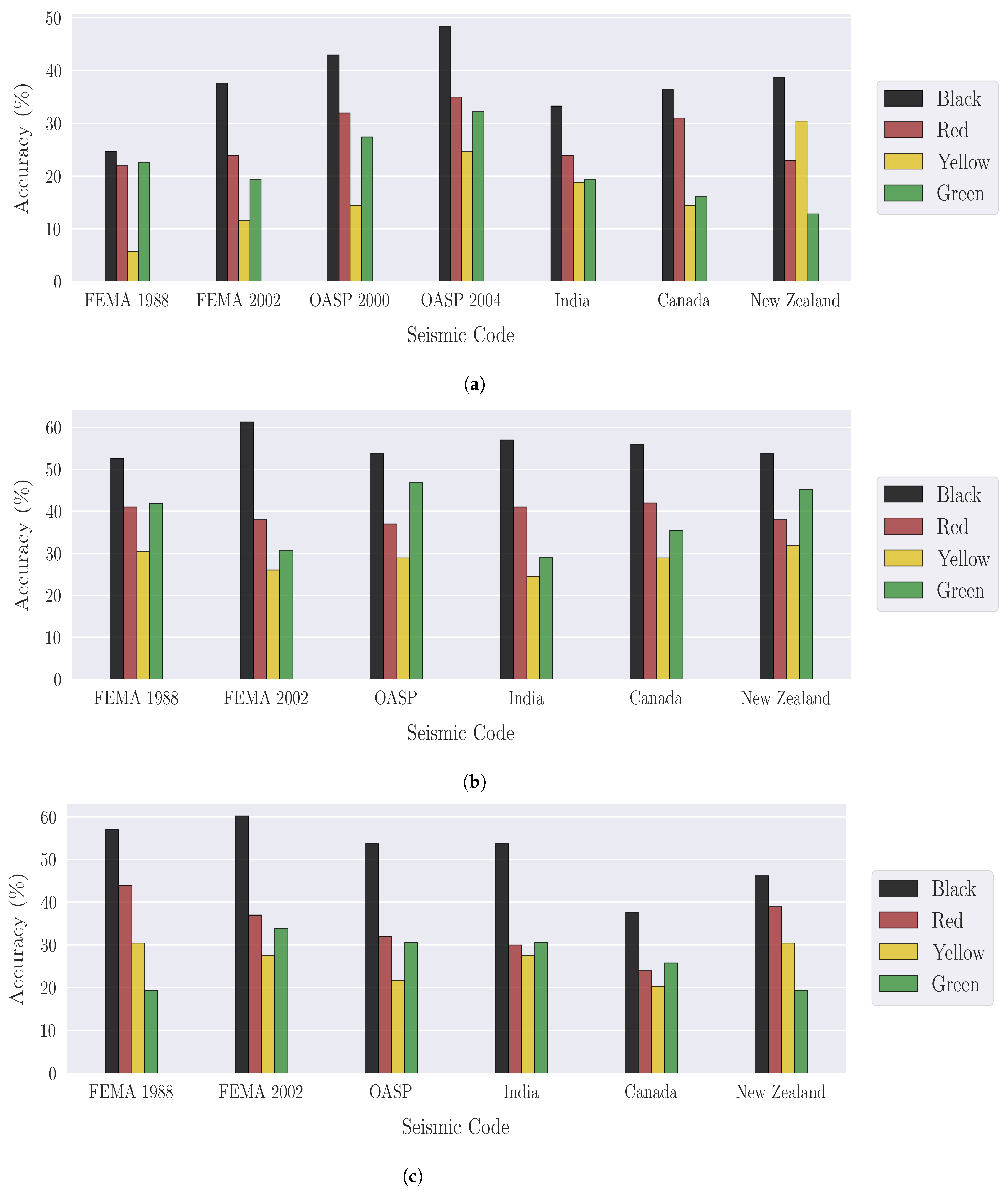
Seismic Code	Bin Accuracy (%)
	Black	Red	Yellow	Green
FEMA 1988	24.73	22.00	5.80	22.58
FEMA 2002	37.63	24.00	11.59	19.35
OASP 2000	43.01	32.00	14.49	27.42
OASP 2004	48.39	35.00	24.64	32.26
India	33.33	24.00	18.84	19.35
Canada	36.56	31.00	14.49	16.13
New Zealand	38.71	23.00	30.43	12.90

,

Table 4. Bin accuracy obtained using the fully trained Machine Learning model.

Seismic Code	Bin Accuracy (%)
	Black	Red	Yellow	Green
FEMA 1988	52.69	41.00	30.43	41.94
FEMA 2002	61.29	38.00	26.09	30.64
OASP (2000 and 2004)	53.76	37.00	28.99	46.77
India	56.99	41.00	24.66	29.03
Canada	55.94	42.00	28.99	35.48
New Zealand	53.76	38.00	31.88	45.16

and

Table 5. Bin accuracy obtained using the proposed recalibrated RVS.

Seismic Code	Bin Accuracy (%)
	Black	Red	Yellow	Green
FEMA 1988	56.99	44.00	30.43	19.35
FEMA 2002	60.22	37.00	27.54	33.87
OASP (2000 and 2004)	53.76	32.00	21.74	30.65
India	53.76	30.00	27.54	30.65
Canada	37.63	24.00	20.29	25.81
New Zealand	46.24	39.00	30.43	19.35

as well as Figure 2, for comparison. It should be reiterated that after undersampling, the dataset contained exactly 100 Red structures ($\left|bi{n}_d^{true}\right|=100$), which is why the corresponding entries in Table 3, Table 4 and Table 5 have integer values.

Comparing the ranking obtained using the established RVS procedures, it can be readily observed that the combination of features with their established weights used in OASP 2000 and 2004 outperformed the other Seismic Codes for this dataset. This improvement in performance was evident for all damage labels. In the label corresponding to collapse (Black), the Codes of New Zealand, FEMA 2002, Canada, and India exhibited slightly lower and comparable performances. It can be observed that, in agreement with the established literature, FEMA 2002 significantly improved over FEMA 1988 in this regard, as the latter exhibited a significantly deteriorated accuracy. Furthermore, it should be noted that a successful ranking should prioritize accuracy in the labels corresponding to “collapse” and “severe damages” (Black and Red, respectively). These are the worst-case damage categories and the most impactful to society. In this regard, all the examined Seismic Codes were successful. In spite of the fact that some performed better than others, the accuracy of the Black bin was significantly higher, with the exception of the FEMA 1988 case, where it was only slightly higher.

We have compared the rankings obtained after running the fully trained Machine Learning models for all the examined Seismic Codes and all the damage categories. We can readily observe that there is a significant increase in the accuracy in all cases. More specifically, the accuracy for the Black class (worst case) was higher than 50% for all employed models. FEMA 2002 achieved a significant accuracy as high as 61%. It should be noted that the same Seismic Code in its current form achieved an accuracy of slightly less than 40% without the use of ML classification algorithms. The models based on the Codes of India, Canada, and New Zealand also exhibited performance improvement. Their accuracy for the Black class bin increased more than 10% with the use of the ML models. OASP exhibited a slight increase of approximately 5% in the accuracy of the Black bin. The highest performance increase for this Code was achieved for the Green class bin, corresponding to buildings that suffered minimal damages. For the Red bin (severe damages), the second most impactful, almost all Seismic Codes exhibited an increase close to 15%. The OASP Code seemed to have benefited the least in this bin as well, with an increase of only 5%. However, it should be reiterated that OASP’s performance was the highest to begin with. Finally, the bin accuracy of the Black label in FEMA 1988 exhibited a noteworthy increase, from approximately 25% to more than 50% when the fully trained ML model was employed.

All of the above clearly indicate the significant benefit of employing ML models for the task of seismic vulnerability ranking. As was demonstrated, using the same features, ML models are capable of learning complex, non-linear relationships that significantly outperform currently established engineering practices.

Finally, we compared the rankings obtained using the proposed ML-based recalibration procedure for RVS. In general, most Seismic Codes benefited from the proposed recalibration, since their accuracy in the most severe damage classes was improved compared to the currently established literature. Furthermore, most of the Codes seemed to have retained high levels of accuracy in the Black and Red bins when compared to the respective scores obtained from the fully trained ML models. On the other hand, most of the loss in accuracy was related to the Green and Yellow bins, which are the least severe and thus the least impactful to society.

The Canadian Code is a notable exception. It exhibited a minimal improvement compared to its currently established form and a considerable loss of accuracy for the Black and Red bins. This is attributed to the fact that the Canadian Code is fundamentally different than the rest. As was mentioned in Section 2.5, most of the examined Seismic Codes are additive, i.e., the computed RVS score is obtained by the summation of (2). On the other hand, the Canadian Code uses summation to obtain a set of intermediate features, which are then multiplied to obtain the final score. The recalibration procedure proposed in this study is linear, which is why it did not fit the Canadian Code as properly as the others.

4. Summary and Conclusions

In the framework of the present study, we have utilized ML-based methodologies to address one of the most severe and impactful engineering challenges; the pre-earthquake seismic vulnerability ranking of a large number of structures within a building stock. As was examined, different countries and organizations have proposed similar yet distinct methodologies. We have examined the approach employed by FEMA (as formulated in 1988 and revised in 2002), India, Canada, New Zealand, and the Greek OASP. As it was shown in Table 2, a different set of features is employed by each of the aforementioned Codes. Even when the same features are used, different weights can be assigned to each of them, based on experts’ opinions. To mitigate this, we have employed a ML-based pairwise methodology, specifically targeting the problem of ranking. More specifically, the Gradient Boosting Machine algorithm was employed to perform comparisons between pairs of structures.

As it can be seen from Table 3 and Table 4, as well as from Figure 2a,b, the proposed methodology was able to outperform currently established engineering practices and to improve on the results obtained with each separate Seismic Code. Regarding the structures that crossed CLS (“Black”), all the examined ML models exhibited an accuracy of over 50%. In some cases, like FEMA 2022 or New Zealand’s Code, we have achieved an accuracy increase between 10 and 20%, compared to the ranking results obtained by the use of the respective Codes’ coefficients. The accuracy improvement for the structures that crossed the ULS (“Red”) was as high as 15% for most of the examined Codes. The performance improved for the other two damage labels as well (moderate—“Yellow”, minimal—“Green”), although these are less impactful than the first two. The above highlight that Gradient Boosting was able to adapt better to the available features and to produce ranking results with higher accuracy and demonstrate its applicability for the task of seismic vulnerability ranking.

Subsequently, the proposed methodology was extended using ML feature attribution techniques, as examined in Section 2.5 and Section 2.6. Inspired by the linearity in which the examined Codes compute their RVS scores, we proposed a linearization of the fully trained ML models using the aggregated metrics of the so-called SHAP values to produce weights similar to the ones employed in a standard RVS procedure. As these values are designed to approximate the behavior of the underlying ML model, we observed that, in most cases, employing this recalibrated and reformulated RVS methodology retained increased performance metrics, compared to the respective currently established approaches.

The benefit of the proposed formulation is that the trained ML models are capable of learning complex, non-linear patterns inherent in the data, which in turn leads to their ability to outperform currently established engineering practices of different countries and organizations. Furthermore, the proposed linearization procedure is also based on the fully trained ML models via the SHAP values feature attribution technique. Thus, even though it inspired by the currently established engineering practices, it provides a basis with which they can be recalibrated to obtain increased accuracy.

Our case study was based on a dataset consisting of real measurements from 457 reinforced concrete structures obtained after the 1999 Athens earthquake. However, given the promising results that were obtained, the proposed methodologies could be expanded. Indeed, different countries and organizations employ different features of interest for pre-earthquake seismic vulnerability ranking in an RVS context. In addition, buildings with different structural types, e.g., masonry buildings commonly found in traditional communities, employ a fundamentally different set of features. Using the respective expanded datasets, individual ML models can be trained for each Seismic Code and structural type, which will be more closely attuned to their individual conditions.

References

- Vicente, R.; Parodi, S.; Lagomarsino, S.; Varum, H.; Silva, J.M. Seismic vulnerability and risk assessment: Case study of the historic city centre of Coimbra, Portugal. Bull. Earthq. Eng. 2011, 9, 1067–1096. [Google Scholar] [CrossRef]
- Lang, K.; Bachmann, H. On the seismic vulnerability of existing buildings: A case study of the city of Basel. Earthq. Spectra 2004, 20, 43–66. [Google Scholar] [CrossRef]
- Federal Emergency Management Agency (FEMA). Rapid Visual Screening of Buildings for Potential Seismic Hazards: A Handbook, 1st ed.; Technical Report; Applied Technology Council: Redwood City, CA, USA, 1988. [Google Scholar]
- Federal Emergency Management Agency (FEMA). Rapid Visual Screening of Buildings for Potential Seismic Hazards: A Handbook, 3rd ed.; Technical Report; Applied Technology Council: Redwood City, CA, USA, 2002. [Google Scholar]
- Brundson, D.; Holmes, S.; Hopkins, D.; Merz, S.; Jury, R.; Shephard, B. The Assessment and Improvement of the Structural Performance of Earthquake Risk Buildings; Technical Report; New Zealand Society for Earthquake Engineering: Wellington, New Zealand, 1996. [Google Scholar]
- Sinha, R.; Goyal, A. A National Policy for Seismic Vulnerability Assessment of Buildings and Procedure for Rapid Visual Screening of Buildings for Potential Seismic Vulnerability; Technical Report; Indian Institute of Technology, Department of Civil Engineering: New Delhi, India, 2002. [Google Scholar]
- Earthquake Planning and Protection Organization (OASP). Provisions for Pre-Earthquake Vulnerability Assessment of Public Buildings (Part A); Technical Report; Greek Society of Civil Engineers: Athens, Greece, 2000. [Google Scholar]
- Foo, S.; Naumoski, N.; Saatcioglu, M. Seismic Hazard, Building Codes and Mitigation Options for Canadian Buildings; Technical Report; Canadian Office of Critical Infrastructure Protection and Emergency Preparedness (CCIPEP): Ottawa, ON, Canada, 2001. [Google Scholar]
- Madariaga, R.; Ruiz, S.; Rivera, E.; Leyton, F.; Baez, J.C. Near-field spectra of large earthquakes. Pure Appl. Geophys. 2019, 176, 983–1001. [Google Scholar] [CrossRef]
- Alhan, C.; Öncü-Davas, S. Performance limits of seismically isolated buildings under near-field earthquakes. Eng. Struct. 2016, 116, 83–94. [Google Scholar] [CrossRef]
- Rossetto, T.; Elnashai, A. Derivation of vulnerability functions for European-type RC structures based on observational data. Eng. Struct. 2003, 25, 1241–1263. [Google Scholar] [CrossRef]
- Eleftheriadou, A.; Karabinis, A. Damage probability matrices derived from earthquake statistical data. In Proceedings of the 14th World Conference on Earthquake Engineering, Beijing, China, 12–17 October 2008; pp. 07–0201. [Google Scholar]
- Yu, Q.; Wang, C.; McKenna, F.; Yu, S.X.; Taciroglu, E.; Cetiner, B.; Law, K.H. Rapid visual screening of soft-story buildings from street view images using deep learning classification. Earthq. Eng. Eng. Vib. 2020, 19, 827–838. [Google Scholar] [CrossRef]
- Ruggieri, S.; Cardellicchio, A.; Leggieri, V.; Uva, G. Machine-learning based vulnerability analysis of existing buildings. Autom. Constr. 2021, 132, 103936. [Google Scholar] [CrossRef]
- Bektaş, N.; Kegyes-Brassai, O. Development in machine learning based rapid visual screening method for masonry buildings. In Proceedings of the International Conference on Experimental Vibration Analysis for Civil Engineering Structures, Milan, Italy, 30 August–1 September 2023; Springer: Cham, Switzerland, 2023; pp. 411–421. [Google Scholar]
- Harirchian, E.; Kumari, V.; Jadhav, K.; Rasulzade, S.; Lahmer, T.; Raj Das, R. A synthesized study based on machine learning approaches for rapid classifying earthquake damage grades to RC buildings. Appl. Sci. 2021, 11, 7540. [Google Scholar] [CrossRef]
- Karabinis, A. Rating of the First Level of Pre-Earthquake Assessment. 2004. Available online: https://oasp.gr/sites/default/files/program_documents/261%20-%20Teliki%20ekthesi.pdf (accessed on 13 May 2024).
- Karampinis, I.; Iliadis, L.; Karabinis, A. Rapid Visual Screening Feature Importance for Seismic Vulnerability Ranking via Machine Learning and SHAP Values. Appl. Sci. 2024, 14, 2609. [Google Scholar] [CrossRef]
- Greek Code for Seismic Resistant Structures–EAK. 2000. Available online: https://iisee.kenken.go.jp/worldlist/23_Greece/23_Greece_Code.pdf (accessed on 13 May 2024).
- Karampinis, I.; Iliadis, L. A Machine Learning Approach for Seismic Vulnerability Ranking. In Proceedings of the International Conference on Engineering Applications of Neural Networks, León, Spain, 14–17 June 2023; Springer: Cham, Switzerland, 2023; pp. 3–16. [Google Scholar]
- Abd Elrahman, S.M.; Abraham, A. A review of class imbalance problem. J. Netw. Innov. Comput. 2013, 1, 9. [Google Scholar]
- Longadge, R.; Dongre, S. Class imbalance problem in data mining review. arXiv 2013, arXiv:1305.1707. [Google Scholar]
- Liu, B.; Tsoumakas, G. Dealing with class imbalance in classifier chains via random undersampling. Knowl.-Based Syst. 2020, 192, 105292. [Google Scholar] [CrossRef]
- Hasanin, T.; Khoshgoftaar, T. The effects of random undersampling with simulated class imbalance for big data. In Proceedings of the 2018 IEEE International Conference on Information Reuse and Integration (IRI), Salt Lake City, UT, USA, 6–9 July 2018; IEEE: New York, NY, USA, 2018; pp. 70–79. [Google Scholar]
- Kumari, R.; Srivastava, S.K. Machine learning: A review on binary classification. Int. J. Comput. Appl. 2017, 160, 11–15. [Google Scholar] [CrossRef]
- Singhal, Y.; Jain, A.; Batra, S.; Varshney, Y.; Rathi, M. Review of bagging and boosting classification performance on unbalanced binary classification. In Proceedings of the 2018 IEEE 8th International Advance Computing Conference (IACC), Greater Noida, India, 14–15 December 2018; pp. 338–343. [Google Scholar]
- Friedman, J.H. Greedy function approximation: A gradient boosting machine. Ann. Stat. 2001, 29, 1189–1232. [Google Scholar] [CrossRef]
- Ganaie, M.A.; Hu, M.; Malik, A.K.; Tanveer, M.; Suganthan, P.N. Ensemble deep learning: A review. Eng. Appl. Artif. Intell. 2022, 115, 105151. [Google Scholar] [CrossRef]
- Kingsford, C.; Salzberg, S.L. What are decision trees? Nat. Biotechnol. 2008, 26, 1011–1013. [Google Scholar] [CrossRef] [PubMed]
- Schapire, R.E. The boosting approach to machine learning: An overview. Nonlinear Estim. Classif. 2003, 171, 149–171. [Google Scholar]
- Pedregosa, F.; Varoquaux, G.; Gramfort, A.; Michel, V.; Thirion, B.; Grisel, O.; Blondel, M.; Prettenhofer, P.; Weiss, R.; Dubourg, V.; et al. Scikit-learn: Machine learning in Python. J. Mach. Learn. Res. 2011, 12, 2825–2830. [Google Scholar]
- Lundberg, S.M.; Lee, S.I. A unified approach to interpreting model predictions. Adv. Neural Inf. Process. Syst. 2017, 30, 4765–4774. [Google Scholar]
- Shapley, L.S. Notes on the n-Person Game: The Value of an n-Person Game; RAND Corporation: Santa Monica, CA, USA, 1951. [Google Scholar]
- Lundberg, S.M.; Erion, G.G.; Lee, S.I. Consistent individualized feature attribution for tree ensembles. arXiv 2018, arXiv:1802.03888. [Google Scholar]
- Lundberg, S.M.; Erion, G.; Chen, H.; DeGrave, A.; Prutkin, J.M.; Nair, B.; Katz, R.; Himmelfarb, J.; Bansal, N.; Lee, S.I. From local explanations to global understanding with explainable AI for trees. Nat. Mach. Intell. 2020, 2, 56–67. [Google Scholar] [CrossRef] [PubMed]
- Kapetana, P.; Dritsos, S. Seismic assessment of buildings by rapid visual screening procedures. Earthq. Resist. Eng. Struct. VI 2007, 93, 409. [Google Scholar]