Article

Design and Evaluation of Face Mask Filtration: Mechanisms, Formulas, and Fluid Dynamics Simulations

by
Francesca Pisapia
1,
David Rees
2 and
Manoochehr Rasekh
2,*
1
Newcells Biotech, The Biosphere, Drayman Helix, South Street, Newcastle upon Tyne NE4 5BX, UK
2
College of Engineering, Design and Physical Sciences, Brunel University London, Uxbridge UB8 3PH, UK
*
Author to whom correspondence should be addressed.
Appl. Sci. 2024, 14(13), 5432; https://doi.org/10.3390/app14135432
Submission received: 15 May 2024 / Revised: 17 June 2024 / Accepted: 19 June 2024 / Published: 22 June 2024
(This article belongs to the Special Issue Research on Environmental Health: Sustainability and Innovation)

Abstract

:
The global adoption of face masks as a preventive measure against the spread of the SARS-CoV-2 virus (COVID-19) has spurred extensive research into their filtration efficacy. This study begins by elucidating various mechanisms of particle penetration and comparing filtration efficiency formulas with experimental data from prior studies. This is compared to the filtration efficiency experimental measurement developed in our previous study. Moreover, it delves into fluid dynamics simulations to examine different turbulent airflow models. Specifically, it contrasts the airflow velocity distribution of the k-ω and k-ε turbulent flow models with that of a quadrant-based average velocity model developed within this research. Furthermore, the study conducts fluid dynamic simulations to assess airflow profiles for six distinct medical and non-medical face masks. The results underscore substantial disparities among the simulations, emphasising the criticality of employing accurate fluid dynamics models for evaluating airflow patterns during diverse respiratory activities such as breathing, coughing, or sneezing, thereby enhancing environmental health in the realm of infectious disease prevention.

1. Introduction

In the past three years, the use of personal protective equipment (PPE) has increased rapidly due to the spread of the severe acute respiratory syndrome coronavirus (SARS-CoV-2, COVID-19). The use of face coverings has been found effective in preventing the transmission of infectious particles between individuals. In general, face masks are considered an effective shield to protect the respiratory system against harmful airborne particles. These particles can be biological organisms (e.g., viruses, bacteria) or man-made, such as industrial emissions [1,2]. PPE is no longer mandatory, but its use is still encouraged in many countries around the world [3,4]. One of the parameters used to determine the performance of a face mask is its filtration efficiency [5]. Filtration efficiency is defined as the ability of a face mask to protect the wearer from the passage of airborne particles [6]. Face masks have different filtration efficiency based on fiber size, morphology (random or ordered structure), pore size, and material weave. Furthermore, air flow velocity and breathing have an impact on filtration efficiency [7,8,9,10]. Therefore, researchers are investigating the fabrication of face masks with high filtration efficiency to decrease the spread of airborne diseases. For instance, Kunda et al. [11] have shown that flow rate and filtration efficacy are inversely proportional, i.e., as the flow rate increases, the filtration efficiency decreases. This behaviour was confirmed by Qian et al. [12] and Richardson et al. [6], who analyzed the relationship between flow rate and particle penetration, showing that these are directly proportional. Therefore, as the flow rate increases, the particle penetration through the mask increases. This phenomenon may occur because high flow rates can enlarge the pore size in a single-layer material, allowing more particles to pass through. Fortunately, the porosity of overlaid face coverings can be restricted by multiple layers of structural orientation and material folding. Previous studies by other scientists demonstrated that layering different filter materials enhanced the filtration efficiency of face masks [13,14]. Typically, face masks have different layers, with each layer having a specific function [15]. In fact, certified masks can have up to six layers (e.g., FFP3) constructed in this manner. There are several established international standards for testing and certifying the filtration efficiency of face masks [16]. However, the advance of computational fluid dynamics (CFD) has made it possible to perform simulations to predict and improve the filtration efficiency of face coverings. Certain computational studies have been published by different researchers, and in most of these studies, the governing equations used were the mass conservation equation of Navier–Stokes coupled with Darcy’s friction law [17]. For instance, Lei et al. [18] simulated air flow over the human face to predict the leakage between the head and the mask. Their research showed that leakage depends on air flow velocity and the viscous resistance coefficient of the filter. Zhang et al. [19] modelled the flow velocity, the carbon dioxide volume fraction, and the temperature distribution inside an N95 face mask using CFD simulation. They found that the temperature and CO2 level within the mask were higher than the ambient level or room temperature. Furthermore, they demonstrated that the flow distribution inside the mask has a cup-shaped pattern, fitting the shape of the N95 facemask.
This study is to find an expression for air flow visualisation and to make a more precise calculation of filtration efficiency. In this paper, the velocity profile is given great accuracy to allow a more quantitative assessment of filtration efficiency for various mask designs. The three-dimensional (3D) profile of velocity distribution for air flow within a rectangular section duct is examined in connection with the filtration efficiency of face masks. The analysis required an assessment of the maximum velocity at the duct centre and the manner in which this falls to zero at the inner duct surfaces. A representation is given based on an elliptical function with a floating magnitude term to represent reflective velocity (laminar and turbulent flow) effects. This has the advantage of a mathematical analysis of the average air flow velocity in connection with filtration efficiency determination. The latter also requires entry and exit velocities on either side of the suspended mask within our air duct design. In this way, a comparison is possible between the efficiencies of approved face masks. It is found that most masks act as an effective barrier, restricting the air flow passage through the fibers by more than 50%. The present theory demonstrated good agreement with the experimental data, confirming that the velocity profile and filtration efficiency calculations precisely predicted how different masks perform. This alignment indicates that there is a significant relationship between the size of the particles and the morphology of the mask fibers. In particular, the mask fibers’ structure effectively filters out particles of varying sizes, and the consistency between theory and experiment underscores the importance of both particle size and fiber morphology in determining how well a mask can filter out contaminants. This connection suggests that optimizing fiber structure could enhance mask filtration efficiency for particles of specific sizes.
Therein, a mask’s design restricts its porosity by layering, orientating, and folding its various layers. Approved masks can have up to six layers (FFP3) constructed in this manner, but normally fewer layers are employed. A range of masks with these properties were investigated [5,9]. This model has the advantage of a mathematical analysis of the average central air flow velocity in connection with filtration efficiency determination. The present analysis is substantiated with physical air flow measurements using pitot tubes located within the air duct on either side of the suspended mask. In this way, it is possible to compare the various efficiencies of approved medical face masks. While standard techniques employ a circular duct, here we use a rectangular duct to suit the face mask profile better (see Figure 1). The rectangular feature required another novel aspect into the study of rectangular air flow modelling.

2. Modelling

The following analysis (Section 2.1, Section 2.2, Section 2.3 and Section 2.4) is based on well-established theory available in the literature (cited) adapted to suit the present investigations.

2.1. Brownian Diffusion

Brownian diffusion is one of the mechanisms by which aerosols penetrate facemasks. Filtration diffusion is based on the random Brownian motion of small particles (diameter less than 0.2 µm) from regions of high concentration to regions of lower concentration. This mechanism is predominant at low air flow velocities. For a face mask, the single-fiber efficiency (ED) is given by the equations below.
E D = 2 · P e 2 / 3
where:
P e = d f   ·   U 0 D
D = k T C C 3 π μ d p
Pe is the Peclet number, d f is the fiber diameter, U0 is the face velocity, D is the diffusion coefficient, k is the Boltzmann constant, T is the temperature of the fluid, μ is the dynamic viscosity of the fluid, dp is the particle’s diameter, and Cc is the Cunningham correction factor [20,21].

2.2. Inertial Impaction

The inertia impaction is defined by Equations (4)–(6) [20]. This mechanism of penetration is predominant with high air flow velocities and large particles (diameter above 0.4 µm). The effect of inertia impaction on the filtration efficiency of a face mask is described by the following equations [21,22]:
E I = S t k · J 2 · K u 2
S t k = ρ p d p 2 C C U 0 18 µ d f
J = 29.6 28 α 0.62 d p d f 2 27.5 d p d f 2.8 if   d p d f < 0.4
where Stk is the Stokes number, Ku is the Kuwabara hydrodynamic factor, ρp is the particle density, and α is the solidity of the filter (fiber packing density). If we assume the J value to be 2, when dp/df is ≥ 0.4, Otherwise, the J value should be determined by Equation (6) [23].

2.3. Interception

An interception phenomenon occurs when a particle following the air flow comes into contact with the filter that captures the particle. This mechanism involves particles in the 0.1–0.4 µm diameter range. The equation below shows the filtering efficiency due to interception [21,24].
E R = 1 α   · R 2 K u · ( 1 + R )  
where R is the defined as dp/df.

2.4. Total Filtration Efficiency

Based on the aforementioned mechanisms of particle penetration, the total single-fiber filtration efficiency is calculated as a combination of each capture mechanism as follows [8]:
E t o t a l = 1 ( 1 E D ) ( 1 E R ) ( 1 E I )
where ED, ER, and EI are the filtration efficiencies due to diffusion, inertia, and interception, respectively. Instead, in our previous study [9], we developed a new method to calculate the filtration efficiency based on the air flow velocity used to test the facemasks. In particular, the filtration efficiency F, expressed as a weighted percentage, was calculated as the difference between the initial (v0) and final velocity (v1) divided by the initial velocity, as shown below. Validation data on filtration efficiency have been included in our recent study [9], where comparisons are made between experimentally obtained filtration efficiency data and those obtained through simulations using our developed formula. The similarity of the results confirmed the reliability of our equation below. We did not include the same results here to avoid redundancy.
F (%) = [(v0/3 − v1)/(v0/3)] × 100%
which is re-written as:
F (%) = [1 − (3v1)/v0)] × 100%

2.5. Mathematical Analysis Based on Laminar Flow Model

The laminar air flow model is characterised by a parabolic velocity profile that spreads far downstream. This type of flow pattern shows few perturbations and turbulence, and it is typical during normal breathing conditions. In our study, we developed a mathematical model described by Equation (10), where a and b are the rectangular aperture half-lengths and x and y are the base coordinates that define the two laminar profiles intersecting at vmax (see Figure 1b). In the model, the velocity profile at entry falls from vmax to zero at the internal wall surfaces. For this, the equation used to describe velocity profiles intersecting at vmax is given by:
V V m a x = 1 x 2 a 2 y 2 b 2 + x a · y b
where the modulus term x a · y b provides the turbulence base profile shown in Figure 1b.

2.6. Quadrant-Based Average Velocity

From the Equation (10), it is possible to obtain an average velocity based upon the maximum central velocity (Vmax) by double integration as follows (Supplementary Materials S1: quadrant-based average velocity):
V = 7 3   a b   V m a x
V ¯ = 7 12 V m a x
Equations (10)–(12) given above were used to simulate the velocity profile distribution using our model in Figure 4c,f.

2.7. Turbulent Flow Model

On the other hand, the turbulent air flow model is usually used to simulate a cough or sneeze. In this type of situation, the exhaled air flow can be divided into two zones: in the first zone, the stream velocity (Ug) is equal to the initial velocity at the source mouth (U0). No turbulence occurs, and the distance from the source (x) is x ≤ 6.2·Dm, where Dm is the mouth diameter, which is assumed to be 2 cm [25]. In the second zone, the distance from the source is x > 6.2·Dm, and the stream velocity has a Gaussian profile distribution described by the equation below [26].
U g = 6.2 · U 0 D m x
The Reynolds number is used to determine the type of flow. In particular, when the Re number is below 2000, the flow is laminar; when 2000 < Re < 4000, the flow is transient; and when Re > 4000, the flow is turbulent [27].
Reynolds number ( R e ) is defined by the Equation (14), where ρ (kg/m3) is the density of the fluid, u is the flow speed (m/s), L is the characteristic linear dimension (m), and µ (Pa·s) is the dynamic viscosity of the fluid.
R e = ρ u L μ      

3. Results and Discussions

Here, we apply the theory given above using CFD simulations adapted to a novel air flow duct apparatus.

3.1. CAD Designs

Based on the air flow models discussed above, Solidworks 2022 (v. SP 2.0, Dassault Systems, Paris, France) was used to draw all the designs shown in Figure 1 below. Figure 1a shows the design and related dimensions of the air duct mask container used to perform the tests illustrated in our previous paper [9]. The air supply is located at the top of the duct, and the pitot tubes, positioned at 7.5 cm on either side, were used to measure the air flow velocity.
The mean velocity volume and the velocity profile obtained using Equation (10) are shown in Figure 1b,c. From the designs below, it appears that for laminar air flow across a rectangular air duct section, the velocity profile is characterised by a parabolic region that spreads far downstream. At entry to the duct (Figure 1b), the quadratic profile seems to admit a degree of turbulence.

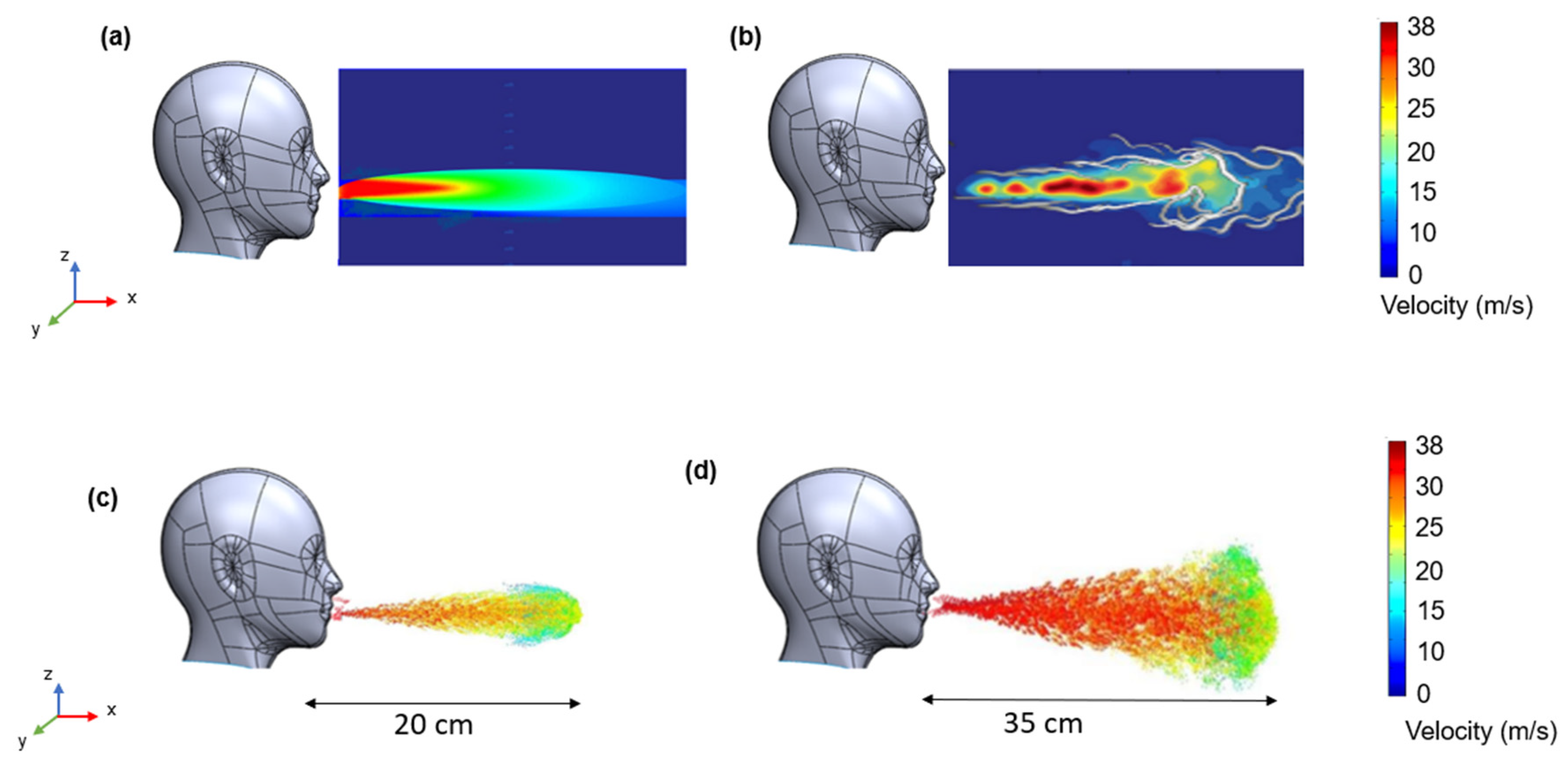
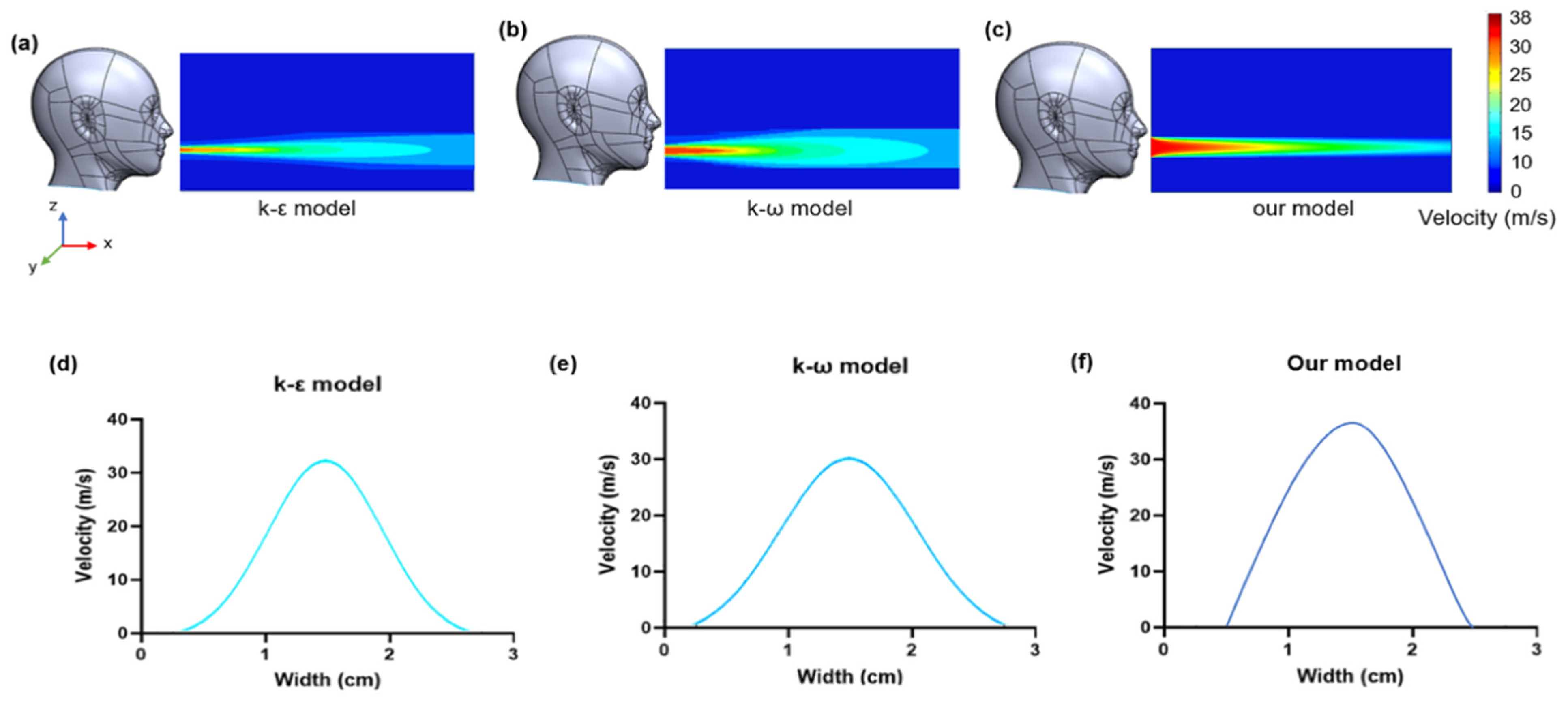
3.2. CFD Simulation Results

Computational fluid dynamics simulations have been carried out using COMSOL Multiphysics (v. 5.6, COMSOL AB, Stockholm, Sweden) in order to give a 3D visualisation of the air flow velocity profile distribution within the air duct (see Figure 2) based on Equation (10). The air flow profile was obtained by creating a cut plane at the desired location in the model. Then, a surface plot was added to the 2D plot group. Finally, a height expression sub-node was added to the surface plot. To perform the simulation, an entry velocity of 38 m/s was chosen based on our previous measurements [9], and the top of the duct was selected as the inlet point. Figure 2a shows a 3D laminar air flow distribution that peaks at 38 m/s on the central access and falls to zero as the air contacts the inner surfaces. It is also assumed that, within the color legend, the velocity partitions into layered stacks with increasing velocity. Figure 2b shows the velocity profile obtained from using the 2D plot feature in COMSOL in combination with Equation (10) when applied to the y-direction.
Subsequently, COMSOL Multiphysics was used to perform CFD simulations to give a flow visualisation of a laminar (see Figure 3a) and turbulent (see Figure 3b) velocity profile contour and to show the respective particle transmission patterns during these two air flow models (see Figure 3c,d). All CFD velocity simulations exclude the presence of the mannequin (see Figure 3a–d). The physical domain comprised the mannequin head, while the external computational domain was reduced to decrease the processing time. The particles were tacked on to trace the air flow trajectory. For the simulations, as a boundary condition, an inlet velocity flow was set to 38 m/s based on our previous study; the ambient temperature was set to 23 °C, while the temperature at the face of the mannequin was set to 32.1 °C, according to the average data obtained from the 12 volunteers [9]. The physical domain is described by the mannequin head, while the external computational domain was reduced to reduce the processing time. This study showed the exhalation phase (t = 3 s) of the breathing cycle to model and visualize the air velocity distribution using the mathematical model developed in this study.
From the simulations, it emerges that for a turbulent air flow model, some particles travel longer distances with a higher velocity compared to particles in laminar air flow. Also, in the turbulent model, the particles tend to disperse into the surrounding environment, as shown in other studies [28,29]. In the laminar flow from the mouth, velocity falls with distance progressively, as the simulation shows and is consistent with Figure 2. But, in the turbulent flow, the velocity distribution is ill-defined, with an island of maximum velocity surrounded by various slower motions with a greater diffusion rate. However, environmental factors such as temperature, relative humidity, and wind affect particle propagation. For instance, Zhao et al. [30] showed that particles travel further in low-temperature, high-humidity environments, while hot, dry environments facilitate particle accumulation. Another study investigated the survival and transmissibility of viruses under different environmental conditions [31]. An additional potential benefit for wearers of masks is that the humidity created within the mask may help combat respiratory diseases such as COVID-19. The results showed that the survival and transmissibility of viruses are high in a low-humidity environment. On the other hand, the transmissibility is low in a highly humid environment. Walker et al. showed [32] that a high level of humidity could limit the spread of viruses to the lungs by stimulating mucociliary clearance (MCC), which is the primary innate defense mechanism of the lung in removing mucus and harmful particles. They showed that a high level of humidity can strengthen the immune system through the secretion of immune signaling proteins such as interferons, which can regulate the fight against viruses.

3.3. Darcy’s Law

Darcy’s law [33] describes the turbulent flow of a fluid through a porous media. This law relates the pressure drop to the velocity. According to the standard physics convention, fluids flow from high-pressure regions to low-pressure regions. In Darcy’s equation, for a turbulent flow through porous media, the pressure drop ∇P due to frictional drag is negatively proportional to the velocity; according to Darcy’s law, “i.e., the negative sign shows that as velocity increases, ∇P decreases”. Therefore, if the ∇P is negative, the flow will be in the positive direction.
P = T f μ k   v
In this equation, ∇P (Pa) is the pressure drop across the filter, Tf is the thickness of the filter (m), k is the permeability coefficient of the filter (m2), µ is the dynamic viscosity of the fluid (Pa s), and v is the face velocity (m/s). Therefore, due to the friction at the inner walls of the duct, the air flow approaches zero near the wall and increases towards the centre of the air duct. According to Darcy’s law, this leads to the formation of a pressure gradient in the same direction as the increasing flow. It should be noted that the permeability of the porous media also plays an important role. In fact, as the porosity of the mask filter decreases, its permeability decreases, and the pressure drop increases [34].

3.4. Brownian Motion Effect

The Brownian motion effect takes place when particle diameters are less than 200 nm. In particular, as particles move in the air, they can be considered a fluid, subjected to two forces, i.e., the inertial force, necessary to generate a variation in the speed of the particles, and the viscous force due to the viscosity of the fluid. The ratio between these two forces is called the Reynolds number (Equation (14)) [27]. Where the COVID-19 particle size ranges from 70 to 90 nm [35,36,37], this means that due to their small size, the inertial force acting on the particles is negligible compared to the laminar force (low Reynolds number). It follows that these particles are subjected to a fluctuating motion, and therefore, they will perform a Brownian motion (stochastic motion). Particle displacement based on Brownian motion is calculated as follows [30]:
x ( t ) = 2 k B T 3 π μ d p t
when k B is the Boltzmann constant (J/K), T is the absolute temperature (K), t is the time (s), μ is the fluid viscosity (Pa·s), and d p is the particle diameter (m). The total particle displacement x at different times (t) is calculated using Equation (16) for a room temperature of 23 °C [9] and d p of 80 nm. The results are shown below (see Table 1).
The results show that Brownian particle motion extends for a long time. This means that COVID-19 particles have a long lifetime since they linger or are suspended in the air for a long time before settling on the ground.

3.5. Prediction from Fluid Flow Mechanics

Navier–Stokes (N-S) equations allow us to predict and compare the behaviour of fluid flow. The main equations are mass and momentum conservation (Supplementary Materials S2: Navier–Stokes equations) [38,39]. Both laminar and turbulent fluid behaviors can be explained by using the N-S equations. However, the phenomenon of turbulence is very complex, and therefore, in order to describe it more simply, turbulence models such as the k-ε and the k-ω are coupled with the N-S equations. These models use turbulent energy dissipation and turbulent kinetic energy factors to provide the time-averaged behaviour of a turbulent fluid [40]. Furthermore, to predict the pressure drop of a fluid passing through porous media (e.g., facemask fabrics) and to simulate the flow resistance through the mask, the following equation was used [28]:
p d f = D   μ f U f 0.5   I   ρ f   U f 2
where (D) is the Darcy viscous coefficient, (I) is the inertial coefficient, and μ f , ρ f and U f are the viscosity, density, and velocity of the fluid, respectively. The Darcy and I coefficients can be estimated according to previous studies [41,42] (Supplementary Materials S3: turbulent flow resistance of porous media). Due to both the Darcy and inertial coefficients, Equation (17) not only takes into account the fluid features (e.g., viscosity, velocity, and density) but also different face mask characteristics such as the fiber diameters, the packing fiber density, and the particle diameter, thus allowing for better prediction accuracy. These properties change the velocity counters for each mask (e.g., in the manner shown in Figure 5).
In this study, we designed and developed a model describing a velocity profile with maximum velocity at the centre (the air duct centre) and a velocity that falls to zero at the inner air duct surfaces. A representation of this model is based on a modulated ellipsoidal function containing a floating term to represent reflective velocity effects. This has the advantage of a mathematical analysis of the average air flow velocity in connection with filtration efficiency determination. COMSOL Multiphysics was used to perform CFD simulations to obtain an overview of the different velocity profiles and contours for the different models discussed above. Again, the initial velocity flow was set to 38 m/s based on the average data in Table 1, the ambient temperature was set to 23 °C, and the temperature at the face of the mannequin was set to 32.1 °C based on the average data obtained from the 12 volunteers [9]. The physical domain is described by the mannequin head, while the external computational domain was reduced to reduce the processing time.
From the simulations above, it emerges that our model (see Figure 4c) generates a larger region with higher velocity (the red region) compared to the k-ω and k-ε models (see Figure 4a,b). Moreover, the model developed in this paper has a high velocity in the centre and a low velocity moving with the x axis from the mannequin mouth (source). As mentioned above, the physical domain included the mannequin head. The externally computational domain (see Figure 4a–c) was reduced to decrease the processing time.
In order to have a better visualisation of the velocity distributions for the three different models, the velocity profiles have been plotted against the width (distance from the mannequin mouth) (see Figure 4d,f). From the velocity profiles above, it emerges that the velocity profile distribution for the k-ε and k-ω models differs from the one obtained for the present model. In particular, for the model presented in this paper, the velocity profile for a rectangular cross section has a parabolic shape, whereas the k-ε and k-ω models have a similar Gaussian velocity distribution for a circular section. When required, the two models described above show a wider velocity distribution, which admits a more accurate prediction of the velocity profile far from the boundary (mannequin mouth). The k-ε model simulates the mean flow features for turbulent flow conditions, primarily for flows with relatively small pressure gradients and high Reynolds numbers. In contrast, the k-ω model captures the effects of turbulent flow conditions and is used for flows with low Reynolds numbers, performing better under adverse pressure gradients. The advantage of using the k-ω model over the k-ε model lies in its greater accuracy in estimating the rate at which flows spread [43,44], although it requires longer computational time to produce a solution. In summary, the k-ε model is more suitable for simulations in indoor environments with low ventilation, while the k-ω model is more reliable for simulating turbulent flow conditions, such as coughing or sneezing [45] in both ventilated indoor and outdoor environments [46].
However, although the k-ε and k-ω models allow a better geometry optimization of the source (mannequin mouth), the two models have been found to overestimate the air flow expansion [47]. On the other hand, the laminar model allows better prediction of the flow behaviour within the entire flow domain.
In our previous study [5], we analyzed the air velocity profile distribution based on the k-ε turbulence model for the six different face masks. In this study, we analyzed the air velocity profile distribution of these masks using the quadrant-based average velocity model (Equation (10)). We simulated the exhalation phase (t = 3 s) of the breathing cycle for modelling and visualizing the air velocity distribution through the face masks by using the mathematical model developed in this study. The pore size data of the masks was measured and used [5] to simulate the air flow resistance. The no-slip boundary condition was applied at the mouth, nose, and forehead of the face mask wearer. For the scope of this study, we did not focus on modeling the shear stress behavior of airflow at these boundaries. Instead, the velocity profile for laminar and turbulent flow were simulated along with temperature influences. An inlet velocity flow based on the quadrant-based average velocity model was considered a boundary condition at the mouth of the mannequin. The external or ambient temperature was set to 23 °C. The initial temperature inside the mask was set at 36.7 °C, and the humidity average was set to 84% based on the average data obtained from the 12 volunteers [9]. The domain was discretized using a grid of tetrahedral cells, with total of approximately 3 × 10⁶ cells. The skewness parameter was evaluated to determine the deviation from the optimal cell size, with a range 0 (ideal) to 1 (worst). In our simulation, the cells exhibited skewness values raging from a minimum of 0.001 to a maximum of 0.80. These simulations showed that the maximum and minimum velocity during the exhalation of six different masks were 2.35 m/s and 0.9 m/s, respectively. The air flow velocity distribution outside the face mask wearer during the exhalation is shown in Figure 5.
The air flow velocity is evenly distributed inside the FFP3 and FFP2 (Figure 5a,b) due to their similar pore sizes (1000 µm and 1600 µm) and fiber diameters (14 µm and 12 µm), respectively. The contour lines showed the disturbance caused by the exhalation of the surrounding air at room temperature into the external domain. The color key shows a range of velocities across the masks. A higher velocity value appears for the Surgical mask (Figure 5c) due to the larger pore size and fiber diameter. The Reusable Cotton, Silk, and Antiviral masks (Figure 5d,f) showed higher air flow velocity. The figure shows that during the exhalation phase, more air passes more quickly through the Silk and Antiviral masks (blue areas in Figure 5e,f). These results correlate with the high pore size and low filtration efficiencies measured for the Silk and Antiviral face masks [5]. Overall, the simulation results obtained using our newly developed model are compatible with the k-ε turbulence model results [1,2,3]. This indicates that both models (k-ε turbulence and quadrant-based average velocity) are suitable for simulating the mask air flow velocity distribution. Alternatively, our symmetrical ellipsoidal surface is sufficiently represented by its quadrant-based formula (Equation (10)). In this paper, we present a new model that is less complex than the k-ε model but equally accurate in simulating the effects of different flow models on air velocity distribution. Our recently published paper [9] simulated the time-dependent temperature distribution for the above six different masks during the berthing cycle at inhalation (t = 3 s) and peak exhalation (t = 1 s). The temperature inside the masks increases during exhalation due to the high temperature of exhaled air, while it remains almost unchanged during inhalation. Different masks exhibit varying behaviors: FFP3 and FFP2 masks show low temperature fluctuations (29–32 °C) but higher temperatures near the nose and mouth (31–33 °C), indicating high resistance to airflow and high filtration efficiency. Surgical and Reusable Cotton masks also show temperature rises during exhalation, particularly around the nose and mouth, but lack high-temperature regions, indicating less airflow resistance. Silk and Antiviral masks show high-temperature areas throughout (30–33 °C), indicating low resistance to airflow. These simulation results align with the velocity profiles and data, confirming the high filtration efficiency of FFP3 and FFP2 masks according to the EN 149 standard [48].
Figure 6 presents a graph based on simulated experimental data obtained in our previous study [9]. The graph shows the temperature distribution inside the face mask while wearing it at the inhalation peak (t = 3 s) and the exhalation peak (t = 1 s) during the breathing cycle. As the temperature of the exhaled air is high, this can increase the temperature inside the mask, whereas during the inhalation phase, the temperature inside the mask remains almost the same. However, different face masks exhibit different behaviors.
Figure 6 indicates that FFP3 and FFP2 masks maintain a high temperature during the exhalation phase, followed by a drop during the inhalation phase. In contrast, Surgical and Reusable Cotton masks exhibit only a small temperature variation between the two phases (approximately 2.5 °C). Meanwhile, Silk and Antiviral masks show a temperature peak during the exhalation phase, followed by a decrease during the inhalation phase.

4. Conclusions

In this study, a description is provided for the various mechanisms of particle penetration across the six different approved face masks. Here, the formula used to calculate the filtration efficiency based on those different mechanisms of particle penetration was compared to the filtration efficiency formula that we developed previously. In addition, this paper evaluates different respiratory airflow dynamic models using CFD simulations. In particular, the velocity profiles were compared with the present model and with the k-ε and k-ω turbulence models. These results demonstrated that particle transmission and velocity profiles are higher in turbulent flow models compared to the more realistic present model. Additionally, in all the models, high-speed flow was observed near the mouth of the mannequin. However, the present model departs from these classical approaches. Here, the velocity profile is described by a parabolic region that spreads far downstream with a maximum velocity at the centre, whereas both turbulent models (k-ε and k-ω) are characterised by a velocity profile that spreads far away from the source. Each model described in this study is suitable for representing respiratory activities. In particular, the turbulent models are useful for describing non-linear or drastic changes in flow gradient. This includes sneezing or coughing, for which the present air flow model is designed to introduce well-defined linear or periodic changes like those that occur during a normal breathing pattern. Finally, it is noted that when SARS-CoV-2 particles leave the humid mouth, they are transported via much larger droplets. It is only after the droplets have evaporated that the SARS-CoV-2 particles released are as small as the particles represented in these simulations.

Supplementary Materials

The following supporting information can be downloaded at: https://www.mdpi.com/article/10.3390/app14135432/s1, Supplementary Material S1–S3.

Author Contributions

Conceptualization, D.R. and M.R.; Methodology, F.P., D.R. and M.R.; Software, F.P.; Validation, D.R. and M.R.; Formal analysis, F.P., D.R. and M.R.; Data curation, D.R. and M.R.; Writing—original draft, F.P., D.R. and M.R.; Writing—review & editing, F.P., D.R. and M.R.; Supervision, M.R. All authors have read and agreed to the published version of the manuscript.

Funding

No funding was received for conducting this study.

Data Availability Statement

The original contributions presented in the study are included in the article; further inquiries can be directed to the corresponding author.

Acknowledgments

The authors would like to thank the Royal Society of Medicine for providing facilities to access the relevant literature. We also thank the Department of Design at Brunel University London for their continuing support.

Conflicts of Interest

The authors declare that the research was conducted without any commercial or financial relationships that could be perceived as potential conflicts of interest.

References

  1. McDonald, F.; Horwell, C.J.; Wecker, R.; Dominelli, L.; Loh, M.; Kamanyire, R.; Ugarte, C. Facemask use for community protection from air pollution disasters: An ethical overview and framework to guide agency decision making. Int. J. Disaster Risk Reduct. 2020, 43, 101376. [Google Scholar] [CrossRef]
  2. Cheng, V.C.-C.; Wong, S.-C.; Chuang, V.W.-M.; So, S.Y.-C.; Chen, J.H.-K.; Sridhar, S.; To, K.K.-W.; Chan, J.F.-W.; Hung, I.F.-N.; Ho, P.-L.; et al. The role of community-wide wearing of face mask for control of coronavirus disease 2019 (COVID-19) epidemic due to SARS-CoV-2. J. Infect. 2020, 81, 107–114. [Google Scholar] [CrossRef] [PubMed]
  3. Rab, S.; Javaid, M.; Haleem, A.; Vaishya, R. Face masks are new normal after COVID-19 pandemic. Diabetes Metab. Syndr. Clin. Res. Rev. 2020, 14, 1617–1619. [Google Scholar] [CrossRef] [PubMed]
  4. Yan, Y.; Bayham, J.; Richter, A.; Fenichel, E.P. Risk compensation and face mask mandates during the COVID-19 pandemic. Sci. Rep. 2021, 11, 3174. [Google Scholar] [CrossRef] [PubMed]
  5. Rasekh, M.; Pisapia, F.; Howkins, A.; Rees, D. Materials analysis and image-based modelling of transmissibility and strain behaviour in approved face mask microstructures. Sci. Rep. 2022, 12, 17361. [Google Scholar] [CrossRef] [PubMed]
  6. Sickbert-Bennett, E.E.; Samet, J.M.; Clapp, P.W.; Chen, H.; Berntsen, J.; Zeman, K.L.; Tong, H.; Weber, D.J.; Bennett, W.D. Filtration efficiency of hospital face mask alternatives available for use during the COVID-19 pandemic. JAMA Intern. Med. 2020, 180, 1607–1612. [Google Scholar] [CrossRef] [PubMed]
  7. Richardson, A.W.; Eshbaugh, J.P.; Hofacre, K.C.; Gardner, P.D. Respirator Filter Efficiency Testing against Particulate and Biological Aerosols under Moderate to High Flow Rates; US Army Edgewood Chemical Biological Center Report for Contract No. SP0700-00-D-3180, Task (335); US Army Edgewood Chemical Biological Center: Edgewood, MD, USA, 2006. [Google Scholar]
  8. Ramarao, B.V.; Tien, C.; Mohan, S. Calculation of single fiber efficiencies for interception and impaction with superposed Brownian motion. J. Aerosol Sci. 1994, 25, 295–313. [Google Scholar] [CrossRef]
  9. Rasekh, M.; Pisapia, F.; Hafizi, S.; Rees, D. Filtering Efficiency and Design Properties of Medical and Non-Medical Grade Face Masks: A Multiscale Modeling Approach. Appl. Sci. 2024, 14, 4796. [Google Scholar] [CrossRef]
  10. Iitani, K.; Tyson, J.; Rao, S.; Ramamurthy, S.S.; Ge, X.; Rao, G. What do masks mask? A study on transdermal CO2 monitoring. Med. Eng. Phys. 2021, 98, 50–56. [Google Scholar] [CrossRef]
  11. Konda, A.; Prakash, A.; Moss, G.A.; Schmoldt, M.; Grant, G.D.; Guha, S. Aerosol filtration efficiency of common fabrics used in respiratory cloth masks. ACS Nano 2020, 14, 6339–6347. [Google Scholar] [CrossRef]
  12. Qian, Y.; Willeke, K.; Grinshpun, S.A.; Donnelly, J.; Coffey, C.C. Performance of N95 respirators: Filtration efficiency for airborne microbial and inert particles. Am. Ind. Hyg. Assoc. J. 1998, 59, 128–132. [Google Scholar] [CrossRef] [PubMed]
  13. O’Kelly, E.; Pirog, S.; Ward, J.; Clarkson, P.J. Ability of fabric face mask materials to filter ultrafine particles at coughing velocity. BMJ Open 2020, 10, e039424. [Google Scholar] [CrossRef]
  14. Brooks, J.T.; Beezhold, D.H.; Noti, J.D.; Coyle, J.P.; Derk, R.C.; Blachere, F.M.; Lindsley, W.G. Maximizing fit for cloth and medical procedure masks to improve performance and reduce SARS-CoV-2 transmission and exposure, 2021. MMWR Morb. Mortal. Wkly. Rep. 2021, 70, 254–257. [Google Scholar] [CrossRef] [PubMed]
  15. Kulmala, I.; Heinonen, K.; Salo, S. Improving filtration efficacy of medical face masks. Aerosol Air Qual. Res. 2021, 21, 200043. [Google Scholar] [CrossRef]
  16. Rengasamy, S.; Shaffer, R.; Williams, B.; Smit, S. A comparison of facemask and respirator filtration test methods. J. Occup. Environ. Hyg. 2017, 14, 92–103. [Google Scholar] [CrossRef]
  17. Tcharkhtchi, A.; Abbasnezhad, N.; Zarbini Seydani, M.; Zirak, N.; Farzaneh, S.; Shirinbayan, M. An overview of filtration efficiency through the masks: Mechanisms of the aerosols penetration. Bioact. Mater. 2021, 6, 106–122. [Google Scholar] [CrossRef]
  18. Lei, Z.; Yang, J.; Zhuang, Z.; Roberge, R. Simulation and evaluation of respirator faceseal leaks using computational fluid dynamics and infrared imaging. Ann. Occup. Hyg. 2013, 57, 493–506. [Google Scholar] [CrossRef] [PubMed]
  19. Zhang, X.; Li, H.; Shen, S.; Cai, M. Investigation of the flow-field in the upper respiratory system when wearing N95 filtering facepiece respirator. J. Occup. Environ. Hyg. 2016, 13, 372–382. [Google Scholar] [CrossRef]
  20. Bai, H.; Qian, X.; Fan, J.; Qian, Y.; Liu, Y.; Duo, Y.; Guo, C.; Wang, X. Microscale layered structural filtration efficiency model: Probing filtration properties of non-uniform fibrous filter media. Sep. Purif. Technol. 2020, 236, 16037. [Google Scholar] [CrossRef]
  21. Monjezi, M.; Jamaati, H. The effects of face mask specifications on work of breathing and particle filtration efficiency. Med. Eng. Phys. 2021, 98, 36–43. [Google Scholar] [CrossRef]
  22. Wang, Q.; Maze, B.; Tafreshi, H.V.; Pourdeyhimi, B. A case study of simulating submicron aerosol filtration via lightweight spun-bonded filter media. Chem. Eng. Sci. 2006, 61, 4871–4883. [Google Scholar] [CrossRef]
  23. Polat, Y.; Calisir, M.; Gungor, M.; Sagirli, M.N.; Atakan, R.; Akgul, Y.; Demir, A.; Kiliç, A. Solution blown nanofibrous air filters modified with glass microparticles. J. Ind. Text. 2021, 51, 821–834. [Google Scholar] [CrossRef]
  24. Zhang, L.; Zhou, J.W.; Zhang, B.; Gong, W. Semi-analytical and computational investigation of different fibrous structures affecting the performance of fibrous media. Sci. Prog. 2020, 103, 0036850419874231. [Google Scholar] [CrossRef] [PubMed]
  25. Wei, J.; Li, Y. Enhanced spread of expiratory droplets by turbulence in a cough jet. Build. Environ. 2015, 93, 86–96. [Google Scholar] [CrossRef]
  26. Lee, J.H.W.; Chu, V. Turbulent Jets and Plumes: A Lagrangian Approach; Springer Science & Business Media: New York, NY, USA, 2012. [Google Scholar]
  27. Wang, C.-S. Airflow in the respiratory system. Interface Sci. Technol. 2005, 5, 31–54. [Google Scholar] [CrossRef]
  28. Dbouk, T.; Drikakis, D. On respiratory droplets and face masks. Phys. Fluids 2020, 32, 063303. [Google Scholar] [CrossRef] [PubMed]
  29. Chen, W.; Zhang, N.; Wei, J.; Yen, H.-L.; Li, Y. Short-range airborne route dominates exposure of respiratory infection during close contact. Build. Environ. 2020, 176, 106859. [Google Scholar] [CrossRef]
  30. Zhao, L.; Qi, Y.; Luzzatto-Fegiz, P.; Cui, Y.; Zhu, Y. COVID-19: Effects of Environmental Conditions on the Propagation of Respiratory Droplets. Nano Lett. 2020, 20, 7744–7750. [Google Scholar] [CrossRef] [PubMed]
  31. Guo, L.; Yang, Z.; Zhang, L.; Wang, S.; Bai, T.; Xiang, Y.; Long, E. Systematic review of the effects of environmental factors on virus inactivation: Implications for coronavirus disease 2019. Int. J. Environ. Sci. Technol. 2021, 18, 2865–2878. [Google Scholar] [CrossRef]
  32. Walker, F.C.; Sridhar, P.R.; Baldridge, M.T. Differential roles of interferons in innate responses to mucosal viral infections. Trends Immunol. 2021, 42, 1009–1023. [Google Scholar] [CrossRef]
  33. Whitaker, S. Flow in porous media I: A theoretical derivation of Darcy’s law. Transp. Porous Media 1986, 1, 3–25. [Google Scholar] [CrossRef]
  34. Mittal, R.; Breuer, K.; Seo, J.H. The Flow Physics of Face Masks. Annu. Rev. Fluid Mech. 2023, 55, 193–211. [Google Scholar] [CrossRef]
  35. Ciofalo, M.; Collins, M.W.; Hennessy, T.R. Modelling nanoscale fluid dynamics and transport in physiological flows. Med. Eng. Phys. 1996, 18, 437–451. [Google Scholar] [CrossRef] [PubMed]
  36. Kim, J.-M.; Chung, Y.-S.; Jo, H.J.; Lee, N.-J.; Kim, M.S.; Woo, S.H.; Park, S.; Kim, J.W.; Kim, H.M.; Han, M.-G. Identification of coronavirus isolated from a patient in korea with COVID-19. Osong Public Health Res. Perspect. 2020, 11, 3–7. [Google Scholar] [CrossRef] [PubMed]
  37. Park, W.B.; Kwon, N.-J.; Choi, S.-J.; Kang, C.K.; Choe, P.G.; Kim, J.Y.; Yun, J.; Lee, G.-W.; Seong, M.-W.; Kim, N.J.; et al. Virus isolation from the first patient with SARS-CoV-2 in Korea. J. Korean Med. Sci. 2020, 35, e84. [Google Scholar] [CrossRef] [PubMed]
  38. White, F.M.; Majdalani, J. Viscous Fluid Flow; McGraw-Hill: New York, NY, USA, 2006; Volume 3, pp. 433–434. [Google Scholar]
  39. Tura, A.; Sarti, A.; Gaens, T.; Lamberti, C. Regularization of blood motion fields by modified Navier–Stokes equations. Med. Eng. Phys. 1999, 21, 27–36. [Google Scholar] [CrossRef] [PubMed]
  40. Zhang, D. Comparison of various turbulence models for unsteady flow around a finite circular cylinder at Re = 20000. J. Phys. Conf. Ser. 2017, 910, 012027. [Google Scholar] [CrossRef]
  41. Jaksic, D.; Jaksic, N. The porosity of masks used in medicine. Tekstilec 2004, 47, 301–304. [Google Scholar]
  42. Jaksic, N.; Jaksic, D. Novel theoretical approach to the filtration of nano particles through non-woven fabrics. In Woven Fabrics; IntechOpen: London, UK, 2012; pp. 205–238. [Google Scholar] [CrossRef]
  43. Anderson, J.D.; Wendt, J. Computational Fluid Dynamics; McGraw-Hill: New York, NY, USA, 1995. [Google Scholar]
  44. Osman, O.; Madi, M.; Ntantis, E.L.; Kabalan, K.Y. Displacement ventilation to avoid COVID-19 transmission through offices. Comput. Part. Mech. 2023, 10, 355–368. [Google Scholar] [CrossRef]
  45. Si, X.A.; Talaat, M.; Xi, J. SARS COV-2 virus-laden droplets coughed from deep lungs: Numerical quantification in a single-path whole respiratory tract geometry. Phys. Fluids 2021, 33, 023306. [Google Scholar] [CrossRef]
  46. Wedel, J.; Steinmann, P.; Štrakl, M.; Matjaž, H.; Jure, R. Can CFD establish a connection to a milder COVID-19 disease in younger people? Aerosol deposition in lungs of different age groups based on Lagrangian particle tracking in turbulent flow. Comput. Mech. 2021, 67, 1497–1513. [Google Scholar] [CrossRef] [PubMed]
  47. Meslema, A.; Bode, F.; Croitoru, C.; Nastase, I. Comparison of turbulence models in simulating jet flow from a cross-shaped orifice. Eur. J. Mech. B/Fluids 2014, 44, 100–120. [Google Scholar] [CrossRef]
  48. EN 149:2001+A1:2009 (E); Respiratory Protective Devices—Filtering Half Masks to Protect against Particles—Requirements, Testing, Marking. European Committee for Standardization (CEN): Brussels, Belgium, 2009.
Figure 1. (a) Design and dimensions of the air duct mask container. (b) Air flow velocity profile for laminar flow model. (c) Mean velocity volume and velocity profile for laminar flow model.
Applsci 14 05432 g001
Figure 2. (a) The 3D and (b) 2D air flow velocity profiles based on laminar flow model.
Applsci 14 05432 g002
Figure 3. CFD simulations of laminar (a) and turbulent (b) velocity profile contours. Particle transmission pattern during laminar (c) and turbulent (d) air flow models. The arrows indicate the distance travelled by the particles.
Applsci 14 05432 g003
Figure 4. CFD simulations of velocity profile contours and respective velocity profile distributions for (a,d) turbulent k-ε model, (b,e) k-ω turbulent model, and (c,f) our model. For all models, the velocity profiles are plotted against the width of the source (distance from the mannequin mouth).
Applsci 14 05432 g004
Figure 5. Velocity profiles during the exhalation phase for FFP3 (a), FFP2 (b), Surgical (c), Reusable Cotton (d), Silk (e), and Antiviral (f) masks.
Applsci 14 05432 g005
Figure 6. A line graph showing the temperature distribution during a breathing cycle, with the exhalation peak occurring at time t = 1 s and the inhalation peak at t = 3 s.
Applsci 14 05432 g006
Table 1. Particle displacement at different time durations.
Time (s)Δx (m)
603 × 10−5
9001 × 10−4
18001.5 × 10−4
27001.8 × 10−4
36002.1 × 10−4
Disclaimer/Publisher’s Note: The statements, opinions and data contained in all publications are solely those of the individual author(s) and contributor(s) and not of MDPI and/or the editor(s). MDPI and/or the editor(s) disclaim responsibility for any injury to people or property resulting from any ideas, methods, instructions or products referred to in the content.

