A New AI Approach by Acquisition of Characteristics in Human Decision-Making Process

Abstract

Planning and decision making are closely interconnected processes that often occur in tandem, influence and informing each other. Planning usually precedes decision making in the chronological sequence, and it can be viewed as a strategy to make decisions. A comprehensive planning or decision strategy can facilitate effective decisions. Thus, understanding and learning human decision-making strategies has drawn intensive attention from the AI community. For example, applying planning algorithms into reinforcement leaning (RL) can simulate the consequence of different actions and select optimal decisions based on learned models, while inverse reinforcement learning (IRL) learns a reward function and policy from expert demonstration and applies them into new scenarios. Most of these methods work based on learning human decision strategies by using modeling of a Markovian decision-making process (MDP). In this paper, we argue that the property of MDP is not fit for human decision-making processes in the real-world and it is insufficient to capture human decision strategies. To tackle this challenge, we propose a new approach to identify the characteristics of human decision-making processes as a decision map, where the decision strategy is defined by the probability distribution of human decisions that are adaptive to the dynamic changes in the environment. The proposed approach was inspired by imitation learning (IL) but with fundamental differences: (a) Instead of aiming to learn an optimal policy based on expert’s demonstrations, we aimed to estimate the distribution of decisions of any group of people. (b) Instead of modeling the environment by an MDP, we used an ambiguity probability model to consider the uncertainty of each decision. (c) The participant trajectory was obtained by categorizing each decision of a participant to a certain cluster based on the commonness in the distribution of decisions. The result shows a feasible way to capture human long-term decision dependency, which provides a complement to the existing machine learning methods for understanding and learning human decision strategies.

1. Introduction

Planning and decision making have been extensively studied in the AI community, with the aim to design and develop an intelligent agent that can interact and act in a variety of environments involving individuals or agents. Planning and decision making are closely related processes. Effective decision making often relies on some form of planning, where individuals or agents consider different options, anticipate potential consequences, and evaluate trade-offs before making a choice. In other words, planning can be viewed as a higher-level cognitive process that supports decision making by providing a structured framework for considering alternatives, setting goals, and organizing actions in pursuit of desired outcomes.

Planning or decision strategies refer to the approaches that individuals use to make decisions [1]. These strategies can vary based on factors such as the decision context, available information, preferences, and cognitive biases [2]. Common decision strategies include heuristic-based approaches (e.g., using rules of thumb or shortcuts) [3], analytical approaches (e.g., systematic analysis of options) [4], and intuitive approaches (e.g., relying on gut feelings) [5]. In other hand, decision making involves various cognitive processes, including perception, attention, memory, reasoning, and judgment. Decision making is also influenced by environmental factors, such as social norms, situational context, available resources, and external constraints. IL is a machine learning approach where an agent learns to perform tasks by observing and mimicking demonstrations provided by an expert. The goal is to replicate the expert’s behavior based on observed actions and outcomes [6]. In IL, the state space and action space are critical components, where the state space encapsulates the environment’s current condition, and the action space defines the agent’s possible decisions or behaviors in response to different states. Imitation learning methods often incorporate planning algorithms to enhance decision-making capabilities. For example, RL techniques combined with planning (such as model-based RL) can enable agents to simulate outcomes of different actions and select optimal decisions based on learned models [7,8]. Planning can also aid in generalization and adaptation in imitation learning settings. Agents can use planning to infer strategies or policies underlying expert demonstrations and apply similar decision-making principles to new scenarios [9]. By integrating planning with imitation learning, agents can exhibit more flexible and robust decision-making behavior, allowing them to handle complex tasks and adapt to changing environments beyond the specific demonstrations they were trained on.

Regarding the different methodologies for reproducing the expert behavior, IL can be generally divided into two major approaches: behavior cloning (BC) and IRL. BC simply tackles the IL problem as a supervised learning problem that aims to build a straightforward mapping from the state space to the action space under the learned policy. But this method can only provide relatively acceptable performance in environments that are the same or similar to the training dataset due to the property of an MDP. However, minor errors can quickly compound when the learned policy departs from the observed states in the demonstration [10]. To increase the awareness of the environment dynamics, an IRL approach uses reinforcement learning methods to extract a reward function based on the optimal expert trajectory and learning a policy from the inferred reward function. However, the IRL method is hardly implemented into real-world tasks since recovering a reward function requires intensive interactions with an external environment, which can be costly in terms of computation and safety [11,12]. Decision making is performed as the center of human interaction with the real world and the decision-making process has a tight relationship with individual characteristics, which was mentioned in our previous work [13]. In this paper, we propose an approach to characterize human decisions. Generally defining the characteristics of decision making may involve understanding the decision strategies employed by individuals or groups in different contexts and examining how the cognitive processes interact to influence decision outcomes. Additionally understanding how the environmental factors shape decision-making behavior can contribute to defining its characteristics. The characteristics of decision making can also be defined in terms of decision outcomes, such as the quality of decisions, decision confidence, decision speed, and decision consistency. Analyzing these outcomes can provide insights into the underlying characteristics of decision-making processes.

The characteristics of decision making can be inferred from analyzing the probability distribution of a group of people’s decisions. Let us break down how this can be achieved:

• Tendency and preference: Analyzing the probability distribution allows us to identify tendencies and preferences within a group. For example, if a certain option is chosen more frequently than others, it suggests a preference for that option within the group [14,15].
• Variability and consensus: The spread or variability of decisions within the probability distribution provides insights into the level of agreement or disagreement between decision makers. A narrow distribution indicates a high level of consensus, whereas a broader distribution suggests greater variability in decision preferences [16,17].
• Decision biases: Certain decision biases may manifest as skewed or asymmetric probability distributions. For instance, if decisions tend to cluster around a particular option due to an anchoring bias or status quo bias, it will be reflected in the shape of the probability distribution [18].
• Risk preferences: Decision making often involves trade-offs between risks and rewards. By analyzing the probability distribution of decisions, we can infer the risk preferences of the group. A risk-averse group may exhibit a probability distribution skewed toward safer options, while a risk-seeking group may display a distribution skewed toward riskier alternatives [19,20].
• Decision stability: The stability of decision making over time can also be assessed through changes in the probability distribution. A consistent probability distribution indicates stable decision-making behavior, whereas fluctuations or shifts in the distribution may signify changes in preferences or external influences [21,22].

While analyzing the probability distribution of decisions provides valuable insights into the characteristics of decision making within a group, it is essential to complement this analysis with other approaches to gain a comprehensive understanding. Factors such as decision strategies, cognitive processes, individual differences, and environmental influences also play significant roles in shaping decision-making behavior. Therefore, a holistic approach that integrates various methods and perspectives is often necessary to fully define the characteristics of decision making.

Our insight is that the difficulty of environment dynamics with previous IL approaches arises from the method for the extraction of human knowledge or experience, i.e., the dynamics of the environment are modeled by an MDP that assumes the next state only depends on the decision (or action) in the current state in the expert trajectory. Thereby, we argue that the extracted human knowledge or experience under MDP settings can only perform well in the low-level task, e.g., object manipulations, where the environmental dynamics are limited. Meanwhile, it is prone to failing in a high-level task, e.g., driving on the highway, which requires high-level knowledge that refers to planning, causal reasoning, or analogical reasoning to handle the environment dynamics. In reality, when human agents use this high-level knowledge to make decisions, they usually consider a long-term relationship, such as what they experienced and what decisions were made. However, MDP settings usually fail to extract such long-term relationships lying in the demonstration data [23,24].

In this paper, we propose a method to extract human knowledge based on the characteristics of decision-making processes from a group of people. This method was inspired by IL but with some fundamental differences: (a) Instead of aiming to learn an optimal policy based on demonstrations, we aimed to estimate the distribution of decisions of a group of people. (b) Instead of modeling the environment by an MDP, we used an ambiguity probability model to consider the uncertainty of each decision. (c) The participant trajectory was obtained by categorizing each decision into a certain cluster based on the commonness compared with the distribution of decisions.

The rest of the paper is organized as follows: the related works are described in Section 2; the challenges in imitation learning are elaborated in Section 3; the proposed method is explained with an application example in Section 4; the results of application example are discussed in Section 5; conclusion and future work are given in Section 6.

2. Related Works

In past decades, the classical AI, known as the good old-fashioned artificial intelligence (GOFAI), has shown itself as powerful and efficient when considering numerous applications [25,26,27]. The GOFAI-based systems supported or even outperformed humans in specific tasks that used to be dominated by human intelligence, for example, IBM’s Deep Blue first defeated the world champion player in the epic chess battle rematch in 1997 [28], and more recently, Google’s AlphaGo system was reported to produce remarkable results in the series of competition with professional Go players from 2015 to 2017 [29]. However, these complicated and challenging problems are considered to be just a fragment of human intelligence in dealing with finite, deterministic, and constrained problems that are a part of the complex and multidimensional intelligence problem spaces [30]. Let us take the board game of checkers as an example. Despite the complexity of the game, which can contain nearly 500 billion possible position moves, it still has a finite number of combinations and a certain number of parameters (i.e., pieces on the board). Besides this, the most important thing is that the board game has fixed rules and perfect information, which means players have insight into everything that has happened before they decide to move a piece. However, unlike these finite, deterministic, constrained board gaming spaces, the real world where humans live are full of uncertainties and usually with limited availability of information for making decisions. Unfortunately, the classical AI tends to fail in pursuing human-level intelligence to deal with problems that are highly dynamic and uncertain. Generally speaking, classical AI has been successful in those tasks that are normally considered difficult, such as playing chess, applying rules of logic, proving a mathematical theorem, or solving certain abstract problems, but fail in those tasks where human actions are experienced as natural, effortless, and dynamic, such as seeing, hearing, talking, walking, and driving; all these skills require common sense [31]. Thus, building systems that incorporate the common sense knowledge became the goal for many classical problem-solving systems, such as CYC (stands for encyclopedia) [32], with the aim to make inferences based on a database of common sense, or the DARPA (Defense Advanced Research Project Agency) project in [33], which is trying to build a machine that can learn by reading a text. However, the successes of these projects are disputed because they are incapable of dealing with common sense in a flexible and adaptive way. One of main reasons is that such systems represent and manipulate the common sense knowledge in an explicit way. For example, in the CYC system, the building blocks of common sense knowledge are propositional statements, such as “cars cannot fly”, “viruses cause infection”, “smoking is harmful to health”, etc.; it is believed that the large collection of such logic-based statements in conjunction with a set of inference rules is all that is needed to represent common sense knowledge. However, common sense is not rigid but highly dynamic and varies in relation to people’s characteristics and background, especially when it refers to the trivial matters in our daily lives [34,35]. For example, we all have an intuitive understanding of the word “driving” that will come to mind if we freely associate with “driving”. It might be turning the wheel, stepping on the gas, a luxury car, a road journey, a car race, the jammed traffic, etc. It is these kinds of variational experiences that form the basis of our common sense, which can never be captured or modeled by such a set of logical statements and rules but requires interactions with the real world.

Common sense reasoning presents challenges in formalization and computational modeling due to its inherent complexity and context-dependent nature. Incorporating common sense into machine learning algorithms, including imitation learning, requires effective representation and integration with data-driven approaches. On the other hand, leveraging common sense can enhance the capabilities of imitation learning agents in addressing real-world tasks that involve rich contextual understanding, intuitive decision making, and adaptive behavior. Integrating common sense reasoning with imitation learning opens up new avenues for developing human-like intelligent systems. Many studies were conducted to explore the relationship between common sense and decision making in different fields, such as managerial decisions in organization [36], integrating common sense as prior knowledge in reinforcement learning [37], and medical decisions in treatment [38]. However, that research put more focus on how common sense as ”practical judgement” influences a decision rather than how common sense is captured as knowledge from lived experience. Despite the fact that in our daily lives, most decision problems are trivial without general agreed-upon criteria, individuals make decisions based on their own perceptions and personality, which are formed by their life experience. This kind of common sense is highly dynamic to different groups of people, and it cannot be simply formalized by a set of rules but requires observations of how individuals interact with the real world and what are the characteristics in those interactions.

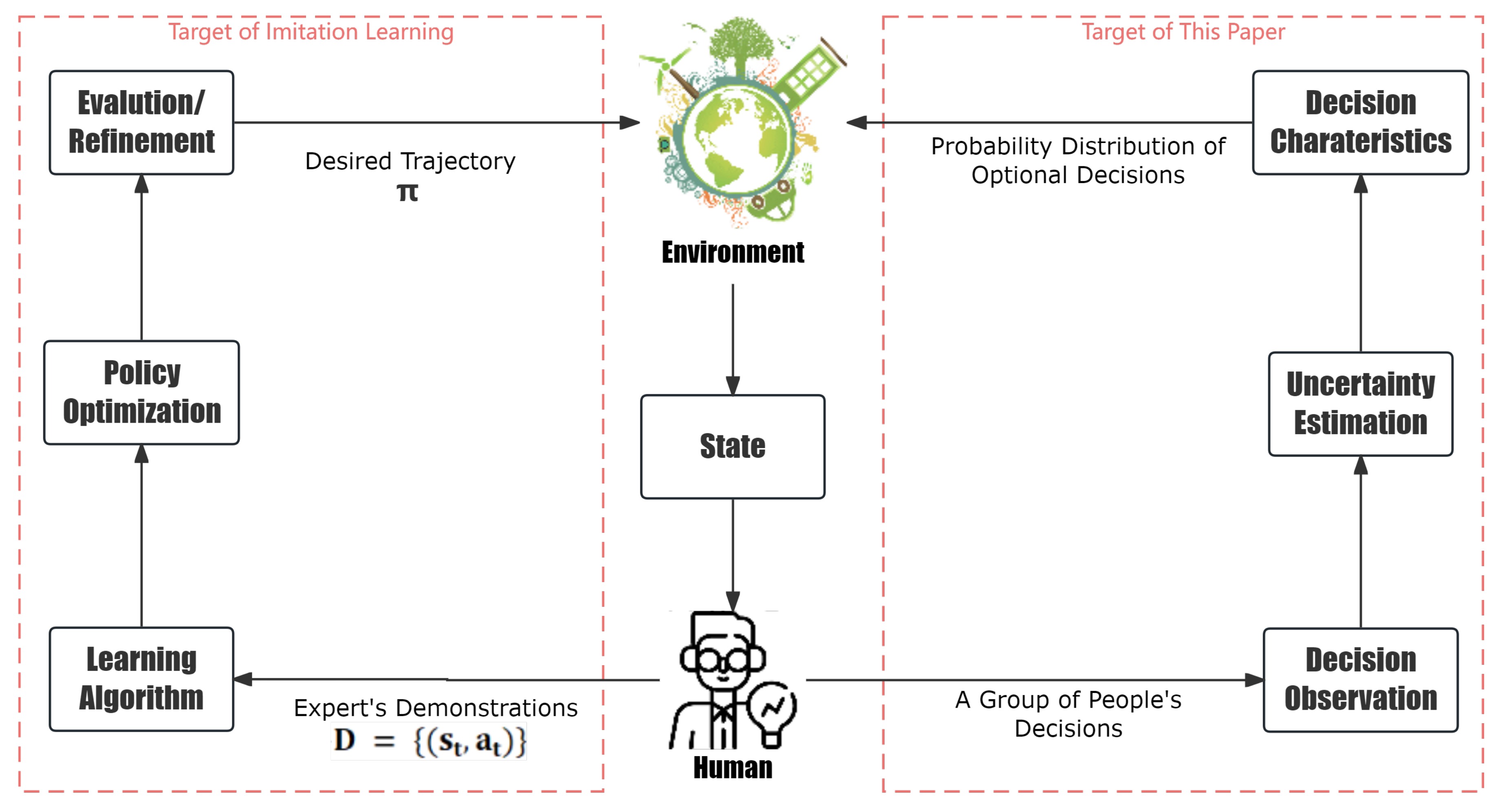
3. Challenges in Imitation Learning

IL as learning from demonstration or apprenticeship learning is generally mathematically formulated within the framework of reinforcement learning [39]. The goal of imitation learning is to enable an agent to mimic expert behavior by learning from observed demonstrations. The following notations are used:

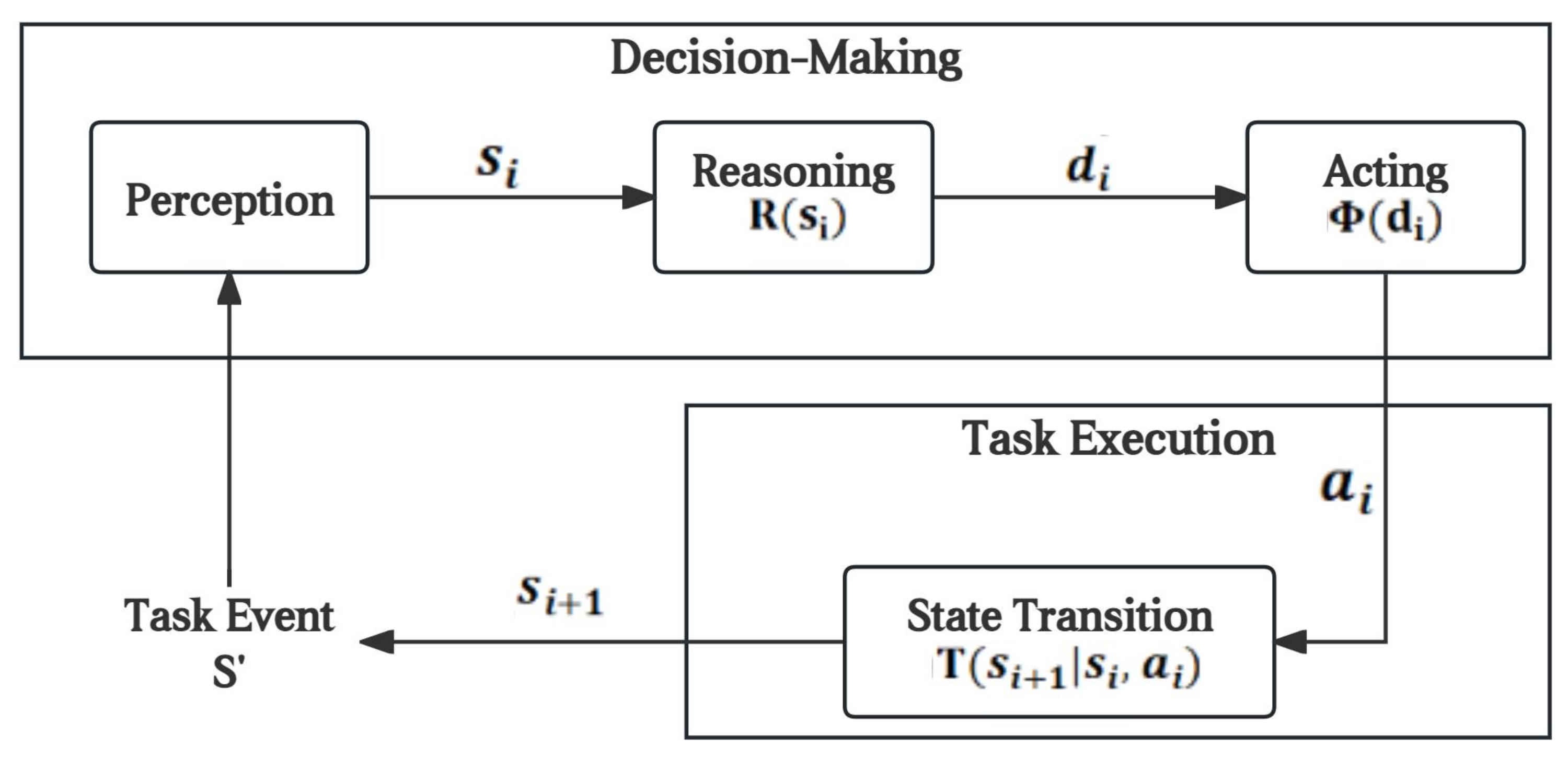
• State space: S, set of all possible states.
• Action space: A, set of all possible actions.
• Reward function: $R:S\times A\to \mathbb{R}$, defines the immediate reward for taking an action in a state.
• Demonstration dataset: $D=\{(s_1,a_1),(s_2,a_2),\dots ,(s_t,a_t)\}$, set of state–action pairs from expert demonstrations.
• Policy: $\pi :S\to A$, agent’s policy mapping states to actions.

The objective of IL is to learn a policy $\pi$ that mimics the expert’s behavior, as demonstrated in D, where the aim is to find a policy $\pi$ that maximizes the expected cumulative reward, like RL but without direct interaction with the environment. In the BC approach, a policy $\pi$ is directly learned that maps state s to action a based on the observed demonstrations [40]. The learning objective of BC can be formulated as minimizing the expected loss between the actions predicted by $\pi$ and the actions in the demonstration dataset D according to

$$mi{n}_{\pi }{\mathbb{E}}_{s\sim D}\left[loss(\pi \left(s\right),a)\right].$$

(1)

Here, $loss$ is a suitable loss function (e.g., mean squared error or cross-entropy) that measures the discrepancy between the predicted action $\pi \left(s\right)$ and demonstrated action a. In the inverse reinforcement learning (IRL) approach, the agent infers the underlying reward function R from the expert’s behavior and then learns a policy $\pi$ that maximizes this inferred reward [41]. The learning process involves estimating the reward function R based on the observed demonstrations and then optimizing the policy $\pi$ to maximize the expected cumulative reward under this reward function according to

$$ma{x}_{\pi }\sum _{t=1}^T{\mathbb{E}}_{S_t\sim p(.)}[R(s_t,\pi \left(s_t\right)],$$

(2)

where $p(.)$ is the distribution over states encountered during the execution of policy $\pi$.

Considering the training and optimization in IL methods, two major trends can be mentioned: the supervised learning approach and iterative improvement. BC can be framed as a supervised learning problem, where the policy $\pi$ is learned using supervised learning techniques (e.g., neural networks) to minimize the prediction error between $\pi \left(s\right)$ and a from D. Iterative approaches, such as policy iteration or gradient-based optimization methods (e.g., policy gradient), can be employed to iteratively update the policy $\pi$ to maximize the expected reward based on the observed demonstrations.

Three major challenges can be considered in relation to IL, which are as follows [6,10,42]:

• Generalization: one key challenge in imitation learning is generalizing the learned policy $\pi$ to new, unseen situations that may differ from the demonstrations;
• Distribution mismatch: the distribution of states encountered during the policy execution by the agent may differ from the distribution of states in the demonstration dataset D, leading to challenges in effective learning;
• Bias and variance trade-off: balancing bias (due to approximation error) and variance (due to noisy demonstrations) is critical for successful imitation learning.

Various techniques and algorithms can be applied to address challenges and achieve effective imitation learning. However, we believe the difficulty of environment dynamics that can be expressed with common sense problems is the major challenge with IL approaches, which cannot be solved due to their fundamental limitation of using an MDP.

4. Method

In this section, we explain the proposed method and elaborate upon it with a game example as a one-dimensional application of the method. The proposed method was inspired by IL approaches.

Figure 1 illustrates the differences between IL approaches and the proposed method to extract human knowledge or experiences. As shown in the left part of Figure 1, an agent learns a task by observing demonstrations performed by an expert. Generally, it extracts expert knowledge through the three processes of a learning algorithm, policy optimization, and evaluation-refinement process. In the demonstration collection procedure, a set of demonstrations is collected from an expert. These demonstrations typically consist of sequences of states and actions that the expert performs while completing the task [43]. The applied learning algorithm process for different methods, such as BC, IRL, or adversarial structured IL, varies, where the goal is to learn a policy or a mapping from states to actions that mimics the behavior of the expert. In the policy optimization process, the learned policy is optimized to minimize the discrepancy between its behavior and that of the expert. This optimization process may involve techniques such as reinforcement learning or supervised learning, depending on the learning algorithm. In the evaluation-refinement process, the learned policy is evaluated on new data to assess its performance. If the performance is not satisfactory, the process may be iterated by collecting more demonstrations, refining the representation, or adjusting the learning algorithm parameters. As shown in the right part of Figure 1, instead of collecting the expert knowledge decisions of a group of people, our proposed method collects decisions to extract the probability distribution of optional decisions through the three processes of decision observation, uncertainty estimation, and the decision characteristics process. In the following, these three processes are elaborated in detail.

As mentioned in the introduction, decision making is the fundamental human activity for interaction with the real world. Figure 2 shows how individuals generally interact with the outside world through decision making. Let us assume the world consists of a set of infinite task events S, where each task event is a subset of S and is denoted as $S^{\prime }=s_i,i=0\dots n$, where $s_i$ is a state of the task event and n is the number of states, which is determined by the sequence of actions (see Figure 2 bottom). The impact of an action on the state, i.e., the state of a task event, is represented by the state transition function $T(s_{i+1}{s}_i,a_i)$, where the $a_i$ represents the action and occurs according to decision making (see Figure 1 top). The decision making contains three processes: perception, reasoning, and acting. In perception, the state is perceived through the measurements of the current state, such as temperature, velocity, and position, so that the state is perceived by a set of parameters and their values. Note that the perception of state is task-oriented, which means the choices of parameters are related to the task under the decision-making process. For example, normally a driver does not look at the back mirror when the car is driven straight forward, but the back mirror is used when driver needs to change lane or drive in reverse. For succinctness, the “state” is used interchangeably with “perceived state” throughout the text and is denoted by $s_i$. The decision $d_i$ is selected after the perception through the reasoning of alternatives, denoted as the function $R\left(s_i\right)$; this process is mostly based on personal experience and other personal factors, such as preference and emotions [44]. A physical action, denoted by the function $\varphi \left(d_i\right)$, happens after a decision. The states during the task execution keep changing until the task event is accomplished. The number of states and their order within the task event are determined by the sequence of actions. It should be noted that Figure 1 illustrates two types of common sense in conjunction with the relation between the decision making and task execution. Implementing the flow chart in the figure from the top to bottom, i.e., using the function $\varphi \left(R\left(s_i\right)\right)$, the figure represents the first type of common sense, i.e., ”the knack for seeing things as they are, or doing things as they ought to be done”. While, implementing the flow chart from the bottom to top, i.e., estimation of the function $\varphi \left(R\left(s_i\right)\right)$, the figure represents the second type of common sense, i.e., the commonsensical experiences of a group for the execution of a task.

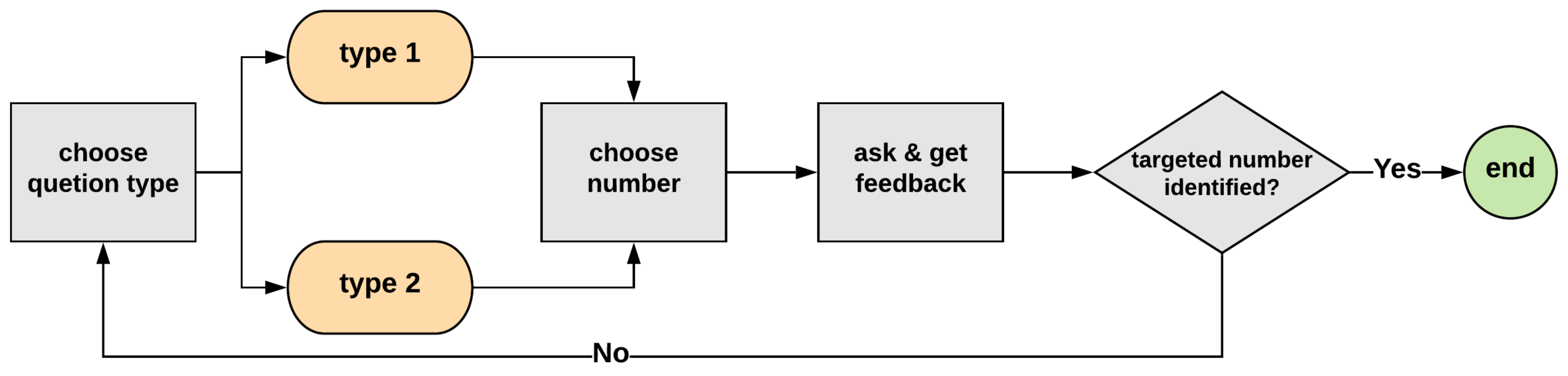
4.1. Application Example

A number-guessing game as a one-dimensional application of the method was designed. The collected data from the game was used to estimate the function $\varphi$ through its inputs $s_i$ and outputs $a_i$, as shown from the bottom to top in Figure 2.

In the game, participants were asked to find out an integer number that was randomly predefined within the range of 1 to 1000. During the task, each participant had unlimited attempts to ask questions to achieve the goal. In each attempt, participants needed to select one of two types of question: (1) Is the next targeted number bigger than participant’s previously chosen number? (2) Is the next targeted number equal to participant’s previous chosen number? Then, an answer of “Yes” or “No” was given to participants based on their questions and chosen number. The task event did not end until the targeted number is identified. The flowchart of the task event is shown in Figure 3. In this task event, the ranges of the targeted number represented states; at the beginning, all participants faced the same state, where the targeted range was from 1 to 1000; after each attempt, the states were changed based on each participant’s actions (i.e., the question and number they chose).

A web-based application was deployed to collect data, and 54 people participated in the game. The decision data of the participants, i.e., the chosen number and type of question, were collected, but only bigger-type question and its chosen number were used in the later data processing since this type of question changed the targeted range more significantly than the other one, especially when the targeted range remained wide in the early phase of task event. In addition, demographic information of the participants was collected as well.

4.2. Method Implementation in Game Application

In this subsection, the usage of the proposed method for the task event processing in the game is explained, where the chosen number $a_i$ and relevant state $s_i$ are processed to estimate the function $\varphi$. The process is achieved in the five steps of normalization, clustering, generation of an ambiguous cluster, and association accumulation.

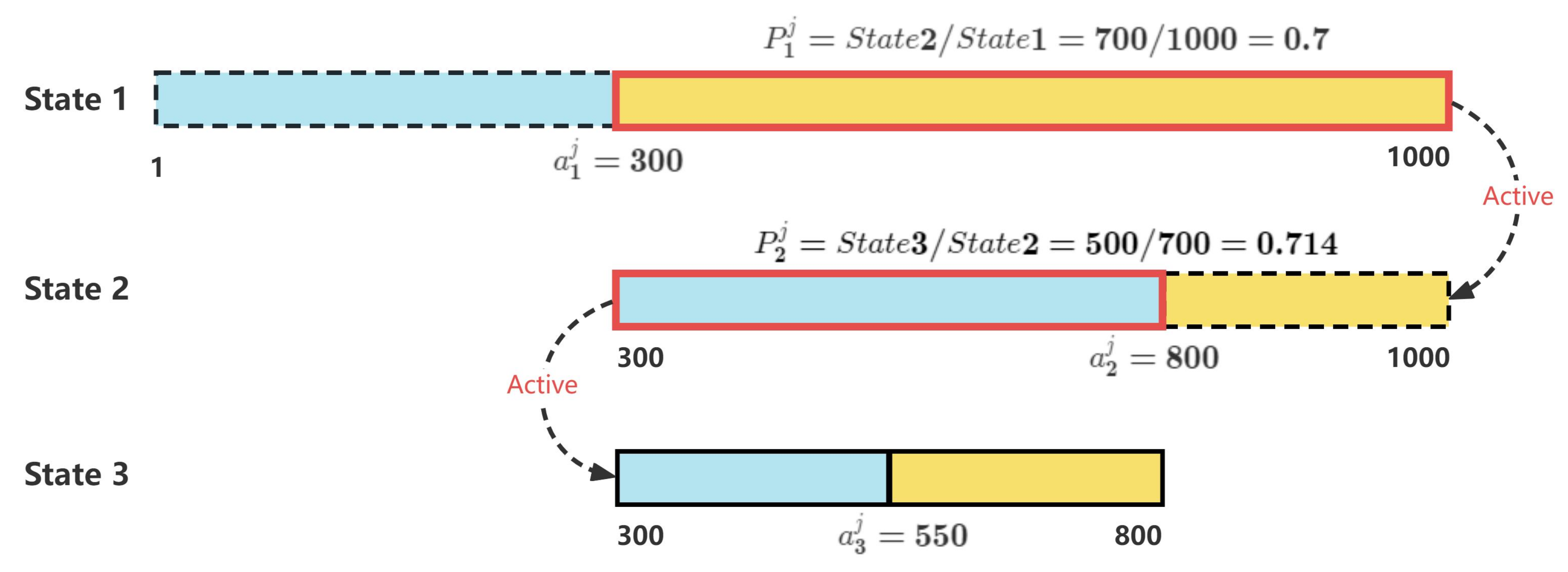
4.2.1. Feature Space Mapping

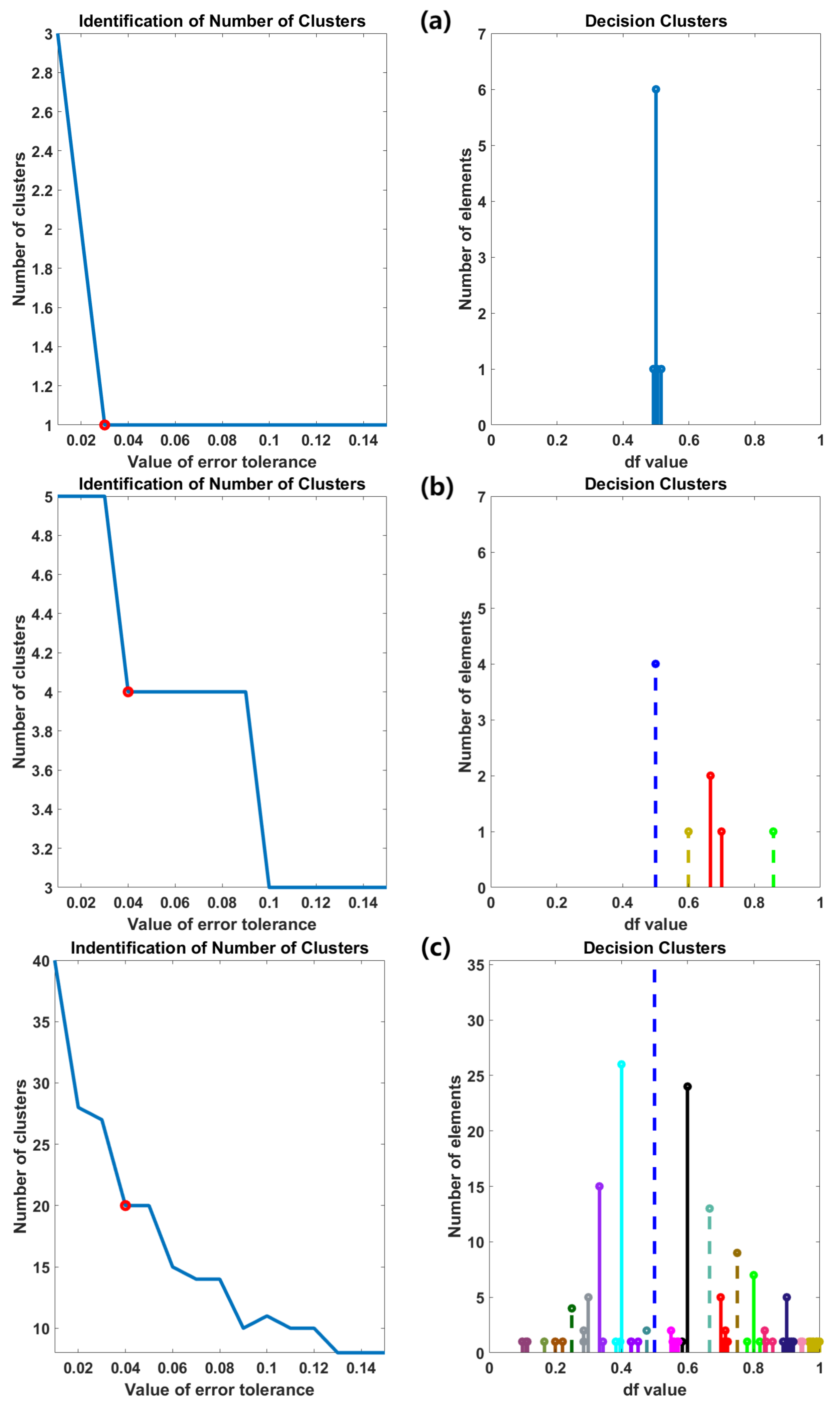
Throughout the execution of task, the decision sequence of each participant was recorded as

$$d_i^j=\{s_i^j,a_i^j\},s_i^j\in S,a_i^j\in A^j$$

(3)

where j is the index of participant; pairs of states and actions were used to represent the decision sequence of each participant. $A^j$ is the set of possible actions of participant j and i is the index of each attempt. The decision sequence of each participant was a consequence of the participant actions, which was executed as

$$d_i^j=\{s_i^j,a_i^j\}\stackrel{T_i^j}{\to }\{s_{i+1}^j,a_i^j\}$$

(4)

which resulted in a new situation of $s_{i+1}^j$. Using the action of each decision as a comparable measurement factor among all the decisions and all the participants created a multiple-measurement space where the decisions of each participant could be considered as one dimension that had a special measurement unit depending on each participant. To be able to compare all the decisions of all the participants a feature space was considered, where the multiple-measurement space was mapped to a one-dimensional feature space according to

$$d_i^j=\{s_i^j,a_i^j\}\stackrel{T_i^j}{\to }\{s_{i+1}^j,a_i^j\}\stackrel{F_i^j}{\to }d{f}_i^j=\{s_i^j,\frac{s_{i+1}^j}{s_i^j},a_i^j{s}_{i+1}^j<s_i^j\}$$

(5)

where F is the feature-mapping operation and $d{f}_i^j$ is the decision in feature space with respect to each decision of a participant given as i and each participant given as j. According to the defined decision in the feature space, the measurable parameter in the feature space became

$$d_i^j=\{s_i^j,a_i^j\}\stackrel{F_i^j}{\to }\left\{p_i^j\right\}$$

(6)

The process of feature mapping is shown in Figure 4, where each participant’s decision sequence was mapped as $d{f}_i^j=\left\{p_i^j\right\}$.

4.2.2. Clustering

The decision sequence of each participant, i.e., $d{f}^j=\left\{p_i^j\right\}$, was clustered as $d{f}^j=\left\{p_{ik}^j\right\}$, where k is the index of the cluster. The clustering method was proposed in two steps. In the first step, the number of clusters for each decision sequence was identified; the result of the clustering was obtained as a one- or multi-element cluster. A one-element cluster is a cluster that includes either only one decision or several decisions but with the same $df$ value, i.e., $C_{one}=\left\{p_{ik}^j\right\},p_{1k}^j=\dots =p_{ik}^j,i=1,\dots ,n$. A multi-element cluster is a cluster that includes at least two varied $d{f}_i^j$ values, i.e., $C_{mul}=\left\{p_{ik}^j\right\},p_{ik}^j\in [0,1],\nexists p_{1k}^j=\dots =p_{ik}^j,i=1,\dots ,n,$$n>=2$. In the second step, all one-element clusters were combined and re-clustered. Details of the two steps are described as follows:

Step 1: K-medoids method [45] was used as core of clustering. Algorithm 1 shows the number of clusters was identified in two sub-steps: (a) A condition was defined to perform k-medoids for constraining the span of each cluster (SEC) less than a threshold, i.e., the value of error tolerance (VET). The SEC was considered to be the distance in each cluster, denoted as $each\_span=p_k^{max}-p_k^{min}$ where $p_k^{max}=max\left\{p_{ik}^j\right\}$ and $p_k^{min}=min\left\{p_{ik}^j\right\}$. VET was increased iteratively from $0.01$ to $0.15$ by steps of $0.01$. Meanwhile, in each iteration, the number of clusters was also increased from one by a one-step manner and continued until the condition $SEC<VET$ was satisfied. Then, the number of clusters regarding each VET was recorded as candidates, denoted as $candi\_num$. (b) The difference between each two sequential candidates was calculated, denoted as $difference=candi\_nu{m}_i-candi\_nu{m}_{i+1}$; the final number of clusters was identical to the first two candidates whose difference was zero. Figure 5a,b shows two examples where the two clustering results in step 1 are presented. On the left of Figure 5, the candidate number of clusters for each VET are plotted and the final number of clusters is marked by the red circle; on the right, the results of clustering according to final numbers of clusters are plotted, where different clusters are distinguished by colors, the one-element clusters are marked by dash lines, and the multi-elements clusters are marked by solid lines.

Step 2: All one-element clusters from all decision sequences of participants were gathered and considered as a new decision sequence of a virtual participant. Then, the ensemble of one-element clusters was re-clustered by using step 1. The result of re-clustering is shown in Figure 5c right.

Algorithm 1: Clustering

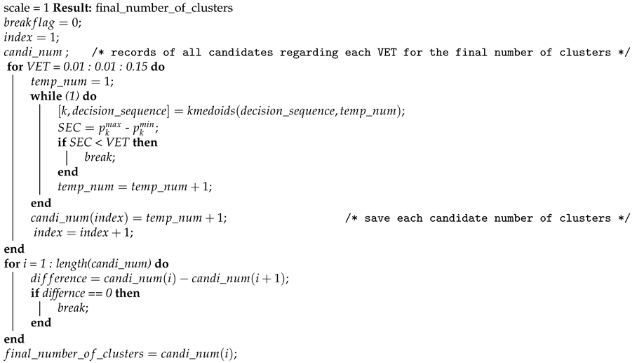
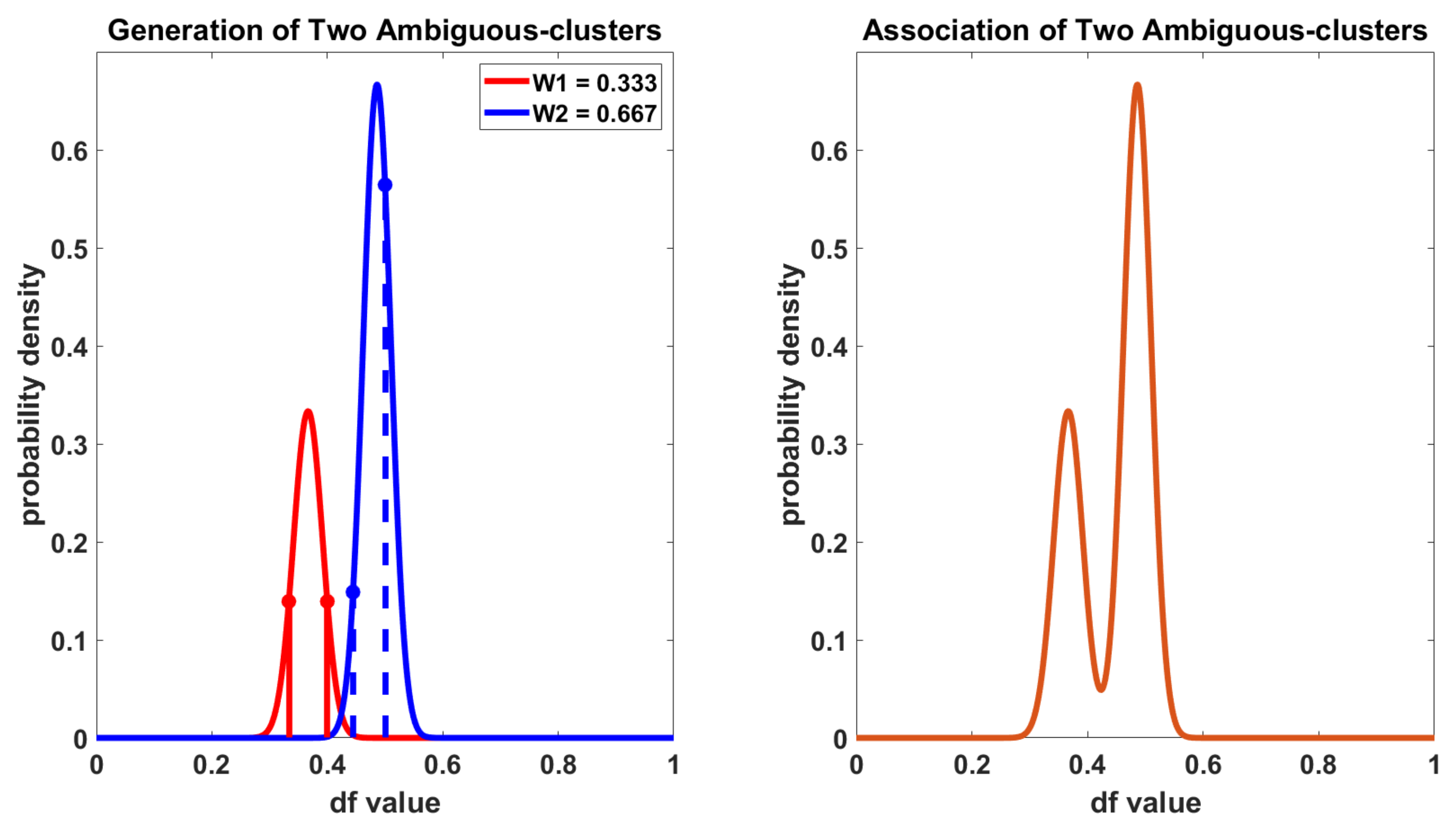
4.2.3. Generation of Ambiguous Clusters

Each cluster was improved to be a more general and analog cluster based on its discrete elements in this process. The improved cluster is called an ambiguous cluster, denoted as ${\psi }_i$, which was achieved by modeling one-element and multi-element clusters as a Gaussian distribution and Student’s t-distribution, respectively. For the Gaussian distribution, the mean was estimated as the value of the element in each one-element cluster; the variance was estimated as half of the relevant VET. For the Student’s t-distribution, the mean and variance were estimated by using the modeling function in Matlab (2021a), i.e., fitdist(x, ‘tLocationScale’), to each multi-element cluster. Due to the limited number of elements (less than 30) in each multi-element cluster, the Student’s t-distribution was used for the estimation rather than using a Gaussian distribution directly. The amplitude of estimated distribution was normalized and weighted by a multiplier factor denoted as ${\lambda }_i$. The factor was determined by the number of discrete elements in each cluster. Examples of generating an ambiguous cluster are shown in Figure 5 left.

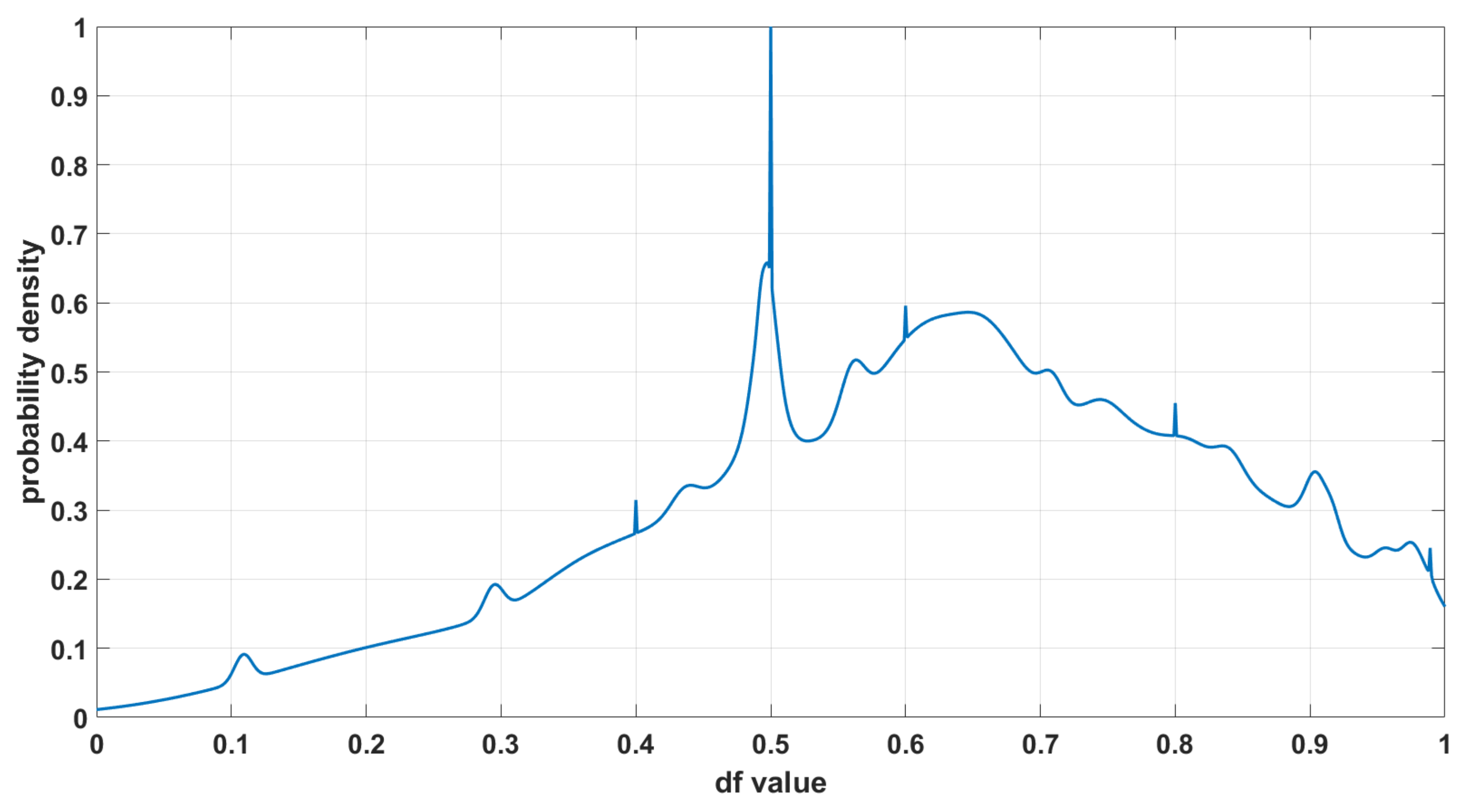
4.2.4. Association and Accumulation

Each two ambiguous clusters were associated by ${\mathrm{\Psi }}_{ij}=W_i{\psi }_i+W_j{\psi }_j$, where ${\mathrm{\Psi }}_{ij}$ is the association of each two ambiguous clusters; i and j were the indexes of the ambiguous clusters; $W_i={\lambda }_i/({\lambda }_i+{\lambda }_j)$, $W_j=1-W_i$, $W_i$, and $W_j$ are the relative weights of two ambiguous clusters in the association. An example of association is shown in Figure 6. Finally, the function $\varphi$ was estimated by accumulating all associations of each two ambiguous clusters, denoted as $\varphi ={\sum }_1^M{\mathrm{\Psi }}_{ij}$, where ${\mathrm{\Psi }}_{ij}$ is the association of each two ambiguous clusters, and $M=n(n-1)/2$ and n are the total numbers of ambiguous clusters.

5. Results and Discussion

The application example and its data processing demonstrated the process of estimating the function $\varphi$ based on the initial decisions made by a group of people. The result of estimation was called a “Decision Map”, where all possible decisions, i.e., initial decisions and their variations, were characterized by a probability distribution, as presented in Figure 7. The amplitude of the probability distribution reveals the commonness among all possible decisions, i.e., a higher amplitude corresponds to more commonness of the decision. The meanings of each process are explained as following: (1) The process of the feature space mapping interpreted the sequence of each participant’s decisions (the chosen number) into a $df$ value in the feature space. The $df$ value indicates how each participant decided to partition the current range to narrow down the searching area of the targeted number for the next attempt. Moreover, the $df$ value is a comparable measurement among all decisions regardless of the dynamic range. (2) To find the common characteristics between those decisions made by each participant, their decision sequence was clustered and each cluster was considered as a decision strategy. For instance, in Figure 5a right, the $df$ values were around 0.5, meaning the participant always used the strategy that partitioned the targeted range at around middle point in each attempt. However, each cluster was just a preliminary representation of a decision strategy that only contained limited decisions, but other possible variations of decision in this strategy might not be observed in the limited attempts during the application example. (3) To include those possible variations of decision into the decision strategies, ambiguous clusters were generated. The generation of an ambiguous cluster was carried out by modeling the uncertainty of initial clusters as a Gaussian distribution or Student’s t-distribution. Note that the choices of modeling type depended on the attribute of initial data in the cluster and subjective preference that had impact on the decision-making process. In this study, the Gaussian distribution and Student’s t-distribution were used for the generation of ambiguous clusters by assuming that possible decisions, i.e., the initial decision and its variations, were normally distributed within a strategy. By generation of an ambiguous cluster, each decision strategy was represented by a probability distribution, where the characteristics of possible decisions within the strategy was reflected by the probability density. Furthermore, the weighting of the normalized ambiguous cluster reflected the commonness of each decision strategy; in other words, the higher-weighted ambiguous cluster meant more inclusions of initial decisions, thereby, the more commonness among decisions was integrated into the relevant strategy. However, each ambiguous cluster only revealed the characteristics of possible decisions within the decision strategy. (4) To understand the characteristics of all possible decisions among the different decision strategies, first, each two ambiguous clusters were associated with their relative weights. As Figure 6 presents, the overlapping part shows the common decisions between two strategies, their amplitudes in the corresponding positions are increased after association. Then, after accumulating all associations of two ambiguous clusters, the commonness of decisions was displayed by amplitudes in the decision map, and the curve also indicated the characteristics of the decision making in this group of people. For example, in Figure 7, the most common decisions were around 0.5; according to this, we can conclude a characteristic of decision making that most participants in this group made decisions cautiously since they preferred to control the consequent risk of decisions (results in the searching ranges in the next attempt) equally.

In addition, the decision map is adaptable to the different groups of people, and it can also indicate the tendency of common decisions as the number of people increases. To investigate this, we divided the dataset of all participants into sub-groups and generated decision maps based on the sub-groups. In each sub-group, participants and their decision data were randomly selected; the number of people increased from 4 to 52 by adding four people each time; and this process of division was repeated 30 times. Figure 8 shows several examples of decision maps based on different sub-groups of participants; each row presents decision maps of sub-groups with a different number of participants; each column presents decision maps of sub-groups with the same number of participants but different individuals. As we can see, the commonness of decisions in the decision maps varied with different numbers of people and different individuals in the sub-groups, but those variations tended to be limited as the number of people grew. Furthermore, the variation in the decision map was measured by $\alpha =\frac{RSS}{TPDM}$, where $TPDM$ stands for the sum of the total population’s decision map (as in Figure 7), and $RSS$ stands for the residual sum of the square betweenthe sub-group’s and total population’s decision maps. The value of $\alpha$ indicates the percentage of difference from the sub-group’s decision map to the TPDM. Figure 9 shows the variations in the decision map with different numbers of people. As shown in the figure, the $\alpha$ values decreased as the number of people grew, especially after 28 people, where an increased number of people made less of a difference on the decision map, which indicates that the commonness contributions of decisions were limited. Moreover, the error bars of the $\alpha$ value reduced, which indicates the random selection of participants had less of an effect on the decision map as the number of people grew.

Another angle of looking at a decision map is its application. Based on the decision map, a one-dimensional ontological structure of decisions (1-DOSE) was applied. Ontology is known as a method to study a concept regarding where and what entities exist and how such entities may be grouped and related to each other [46]. In the 1-DOSE, the concept was regarded as a group of people’s common sense regarding dealing with a specific problem or task; their decisions to solve the problem were regarded as the entities of the concept; the decision strategy was regarded as a groups of entities; and the relationship between strategies was hierarchically connected by ranks.

Table 1. 1-DOSE with 30 decision strategies (identified by cluster index).

Rank	Cluster Index	Rank	Cluster Index	Rank	Cluster Index
1	2	11	9	21	10
2	30	12	28	22	24
3	7	13	20	23	16
4	23	14	17	24	12
5	3	15	22	25	5
6	4	16	29	26	25
7	14	17	15	27	18
8	27	18	1	28	26
9	8	19	13	29	11
10	21	20	6	30	19

shows an example of a 1-DOSE with 30 decision strategies. The rank was calculated in three steps: (1) each strategy’s initial decisions were projected to the corresponding positions in the decision map; (2) the corresponding amplitudes at those positions were accumulated and the accumulated value was assigned to each decision strategy; (3) the ranks of decision strategies were identified based on the sorting of their accumulated values of amplitude in descending order. This rank revealed the hierarchical similarities of decision strategies since the decision strategy with a higher rank meant it had a higher accumulated value of amplitude and its initial decisions were shared by more participants in their decision-making process. Moreover, a 1-DOSE provides a way to quantitatively analyze the characteristics of the decisions made by a person regarding a specific problem or task.

Table 2. The commonness analysis with two participants’ decisions.

Participant 1			Participant 2
Decision Sequence	D.S. Index	Rank	Decision Sequence	D.S. Index	Rank
0.5000	2	1	0.5000	2	1
0.4000	7	3	0.6000	49	57
0.7500	8	9	0.3333	38	91
0.6667	23	4	0.4000	38	91
0.5000	2	1	0.5000	2	1
0.6000	30	2	0.7500	60	45
0.8333	53	75	0.6667	49	57
0.8000	53	75	0.5000	2	1
0.5000	2	1	0.8000	60	45
0.5000	2	1	0.7500	60	45
Sum of ranks		172	Sum of ranks		434

shows an example of such an analysis between two participants. Each $df$ value in their decision sequences was assigned with a rank number; the rank number corresponded to the rank of a relevant decision strategy in the 1-DOSE; the sum of ranks reflects the commonness of the participant’s decision sequence, i.e., a lower sum of the ranks number means more common decisions were made by the participant in his or her decision sequence. In the analysis of Table 2, the participants’ personalities were exposed somehow by how their decisions were close to the common strategy applied by other participants. By using “somehow”, we mean that only one decision sequence was not good enough to evaluate the whole personality of the participant, but it could be considered as one piece of personality itself in a decision-making process. This provides a new perspective for current research of an autonomous decision-making system, where the absence of situation data in reconstructions or modeling used leads to poor or no decision making. By implementation of the 1-DOSE, the dependence between situation reconstruction and decision making can be reduced since humans have contributed to the hard part in the decision-making process, i.e., the process from the perception of the situation to the decision making. The machine only needs to learn how to apply one characteristic of making decisions to a specific problem or task, which can refer to the 1-DOSE. In addition, the 1-DOSE does not necessarily show the optimal decisions, but it always shows an overview of how decisions are made by people related to their characteristics. However, the decision map can be optimized by characterizing a group of experts’ decisions regarding a given problem or task and then the 1-DOSE based on the experts’ decision map can be implemented, where the optimal decisions are aligned with the most common decisions.

6. Conclusions

In this paper, we propose a approach to acquire characteristics of decision making based on a group of people’s decisions regarding a specific task. The idea of this method was inspired by IL, but with fundamental differences: (a) Instead of aiming to learn an optimal policy based on expert’s demonstrations, we aimed to estimate the distribution of decisions of a group of people. (b) Instead of modeling the environment by an MDP, we used an ambiguity probability model to consider the uncertainty of each decision. (c) The participant trajectory was obtained by categorizing each decision of the participant to a certain cluster based on the commonness in the distribution of decisions. The feasibility of the approach was addressed by an application example, where a one-dimensional intelligence problem was designed for data collection. In the processes of applying example data, we used statistical methods to estimate and characterize all possible decisions that could be made by this group of participants. The characteristics of decision making was estimated and represented by a probability distribution called a decision map, where the curve of the amplitude indicates the commonness of decisions within the group of participants. We also discussed the variations in the decision map, which shows the decision map is adaptable to unveil the characteristic of decision making based on different groups of participants. In the end, we discussed a decision-map-based application, named 1-DOSE, which used a group of peoples’ decision map as a reference to measure the commonness of an individual’s decision trajectory. This application provides a new perspective to the research of learning and mimicking human decision making in autonomous systems. However, in this study, the lack of a comparison of the proposed approach with other existing approaches is a shortcoming, which is planned to be investigated in future research work.

References

1. Daniel, K. Thinking, Fast and Slow; Macmillan: New York, NY, USA, 2011. [Google Scholar]
2. Mousavi, S.; Gigerenzer, G. Risk, uncertainty, and heuristics. J. Bus. Res. 2014, 67, 1671–1678. [Google Scholar] [CrossRef]
3. Gilovich, T.; Griffin, D.; Kahneman, D. Heuristics and Biases: The Psychology of Intuitive Judgment; Cambridge University Press: Cambridge, UK, 2002. [Google Scholar]
4. Bazerman, M.H.; Moore, D.A. Judgment in Managerial Decision Making; John Wiley & Sons: Hoboken, NJ, USA, 2012. [Google Scholar]
5. Chen, V.; Liao, Q.V.; Wortman Vaughan, J.; Bansal, G. Understanding the role of human intuition on reliance in human-AI decision-making with explanations. Proc. ACM Hum. Comput. Interact. 2023, 7, 1–32. [Google Scholar]
6. Zheng, B.; Verma, S.; Zhou, J.; Tsang, I.W.; Chen, F. Imitation Learning: Progress, Taxonomies and Challenges. IEEE Trans. Neural Netw. Learn. Syst. 2022, 35, 6322–6337. [Google Scholar] [CrossRef]
7. Edwards, A.; Sahni, H.; Schroecker, Y.; Isbell, C. Imitating latent policies from observation. In Proceedings of the International Conference on Machine Learning, Long Beach, CA, USA, 10–15 June 20109; PMLR: New York, NY, USA, 2019; pp. 1755–1763. [Google Scholar]
8. Nair, A.; Chen, D.; Agrawal, P.; Isola, P.; Abbeel, P.; Malik, J.; Levine, S. Combining self-supervised learning and imitation for vision-based rope manipulation. In Proceedings of the 2017 IEEE International Conference on Robotics and Automation (ICRA), Singapore, 29 May–3 June 2017; IEEE: New York, NY, USA, 2017; pp. 2146–2153. [Google Scholar]
9. Garg, D.; Chakraborty, S.; Cundy, C.; Song, J.; Ermon, S. Iq-learn: Inverse soft-q learning for imitation. Adv. Neural Inf. Process. Syst. 2021, 34, 4028–4039. [Google Scholar]
10. Ding, Z. Imitation learning. In Deep Reinforcement Learning: Fundamentals, Research and Applications; Springer: Berlin/Heidelberg, Germany, 2020; pp. 273–306. [Google Scholar]
11. Finn, C.; Levine, S.; Abbeel, P. Guided cost learning: Deep inverse optimal control via policy optimization. In Proceedings of the International Conference on Machine Learning, New York, NY, USA, 19–24 June 2016; PMLR: New York, NY, USA, 2016; pp. 49–58. [Google Scholar]
12. Ho, J.; Ermon, S. Generative adversarial imitation learning. Adv. Neural Inf. Process. Syst. 2016, 29. [Google Scholar]
13. Zhou, Y.; Khatibi, S. Mapping and Generating Adaptive Ontology of Decision Experiences. In Proceedings of the 3rd International Conference on Information Science and Systems, Cambridge, UK, 19–22 March 2020; pp. 138–143. [Google Scholar]
14. Kuehnhanss, C.R. The challenges of behavioural insights for effective policy design. Policy Soc. 2019, 38, 14–40. [Google Scholar] [CrossRef]
15. Leonard, T.C. Richard H. Thaler, Cass R. Sunstein, Nudge: Improving decisions about health, wealth, and happiness. Const. Political Econ. 2008, 19, 356. [Google Scholar] [CrossRef]
16. Kerr, N.L.; Tindale, R.S. Group performance and decision making. Annu. Rev. Psychol. 2004, 55, 623–655. [Google Scholar] [CrossRef]
17. Boix-Cots, D.; Pardo-Bosch, F.; Pujadas, P. A systematic review on multi-criteria group decision-making methods based on weights: Analysis and classification scheme. Inf. Fusion 2023, 96, 16–36. [Google Scholar] [CrossRef]
18. Tversky, A.; Kahneman, D. Judgment under Uncertainty: Heuristics and Biases: Biases in judgments reveal some heuristics of thinking under uncertainty. Science 1974, 185, 1124–1131. [Google Scholar] [CrossRef]
19. Tversky, A.; Kahneman, D. Advances in prospect theory: Cumulative representation of uncertainty. J. Risk Uncertain. 1992, 5, 297–323. [Google Scholar] [CrossRef]
20. Peterson, J.C.; Bourgin, D.D.; Agrawal, M.; Reichman, D.; Griffiths, T.L. Using large-scale experiments and machine learning to discover theories of human decision-making. Science 2021, 372, 1209–1214. [Google Scholar] [CrossRef]
21. Hardisty, D.J.; Thompson, K.F.; Krantz, D.H.; Weber, E.U. How to measure time preferences: An experimental comparison of three methods. Judgm. Decis. Mak. 2013, 8, 236–249. [Google Scholar] [CrossRef]
22. Tversky, A.; Shafir, E. Choice under conflict: The dynamics of deferred decision. Psychol. Sci. 1992, 3, 358–361. [Google Scholar] [CrossRef]
23. Zhu, Q.; Chen, Y.; Wang, H.; Zeng, Z.; Liu, H. A knowledge-enhanced framework for imitative transportation trajectory generation. In Proceedings of the 2022 IEEE International Conference on Data Mining (ICDM), Orlando, FL, USA, 30 November–3 December 2022; IEEE: New York, NY, USA, 2022; pp. 823–832. [Google Scholar]
24. Zhang, X.; Li, Y.; Zhou, X.; Zhang, Z.; Luo, J. Trajgail: Trajectory generative adversarial imitation learning for long-term decision analysis. In Proceedings of the 2020 IEEE International Conference on Data Mining (ICDM), Sorrento, Italy, 17–20 November 2020; IEEE: New York, NY, USA, 2020; pp. 801–810. [Google Scholar]
25. Abu-Nasser, B. Medical expert systems survey. Int. J. Eng. Inf. Syst. (IJEAIS) 2017, 1, 218–224. [Google Scholar]
26. Behzadian, M.; Otaghsara, S.K.; Yazdani, M.; Ignatius, J. A state-of the-art survey of TOPSIS applications. Expert Syst. Appl. 2012, 39, 13051–13069. [Google Scholar] [CrossRef]
27. Oh, J.; Yang, J.; Lee, S. Managing uncertainty to improve decision-making in NPD portfolio management with a fuzzy expert system. Expert Syst. Appl. 2012, 39, 9868–9885. [Google Scholar] [CrossRef]
28. Campbell, M. Knowledge discovery in deep blue. Commun. ACM 1999, 42, 65–67. [Google Scholar] [CrossRef]
29. Silver, D.; Hubert, T.; Schrittwieser, J.; Antonoglou, I.; Lai, M.; Guez, A.; Lanctot, M.; Sifre, L.; Kumaran, D.; Graepel, T. Mastering chess and shogi by self-play with a general reinforcement learning algorithm. arXiv 2017, arXiv:1712.01815. [Google Scholar]
30. Petrović, V.M. Artificial Intelligence and Virtual Worlds—Toward Human-Level AI Agents. IEEE Access 2018, 6, 39976–39988. [Google Scholar] [CrossRef]
31. Pfeifer, R.; Bongard, J. How the Body Shapes the Way We Think: A New View of Intelligence; MIT Press: Cambridge, UK, 2007. [Google Scholar]
32. Lenat, D.B.; Guha, R.V.; Pittman, K.; Pratt, D.; Shepherd, M. Cyc: Toward programs with common sense. Commun. ACM 1990, 33, 30–49. [Google Scholar] [CrossRef]
33. Olive, J.; Christianson, C.; McCary, J. Handbook of Natural Language Processing and Machine Translation: DARPA Global Autonomous Language Exploitation; Springer Science & Business Media: Berlin/Heidelberg, Germany, 2011. [Google Scholar]
34. Harnad, S. The symbol grounding problem. Phys. Nonlinear Phenom. 1990, 42, 335–346. [Google Scholar] [CrossRef]
35. Shanahan, M. Perception as abduction: Turning sensor data into meaningful representation. Cogn. Sci. 2005, 29, 103–134. [Google Scholar] [CrossRef]
36. Dinur, A.R. Common and un-common sense in managerial decision making under task uncertainty. Manag. Decis. 2011, 49, 694–709. [Google Scholar] [CrossRef]
37. Garnelo, M.; Arulkumaran, K.; Shanahan, M. Towards deep symbolic reinforcement learning. arXiv 2016, arXiv:1609.05518. [Google Scholar]
38. Leventhal, H.; Phillips, L.A.; Burns, E. The Common-Sense Model of Self-Regulation (CSM): A dynamic framework for understanding illness self-management. J. Behav. Med. 2016, 39, 935–946. [Google Scholar] [CrossRef]
39. Abbeel, P.; Ng, A.Y. Apprenticeship learning via inverse reinforcement learning. In Proceedings of the Twenty-First International Conference on MACHINE Learning, Banff, AB, Canada, 4–8 July 2004; p. 1. [Google Scholar]
40. Bain, M.; Sammut, C. A Framework for Behavioural Cloning. In Proceedings of the Machine Intelligence 15, Oxford, UK, 17 July 1995; pp. 103–129. [Google Scholar]
41. Ng, A.Y.; Russell, S. Algorithms for inverse reinforcement learning. In Proceedings of the ICML, San Francisco, CA, USA, 29 June–2 July 2000; Volume 1, p. 2. [Google Scholar]
42. Hussein, A.; Gaber, M.M.; Elyan, E.; Jayne, C. Imitation learning: A survey of learning methods. ACM Comput. Surv. (CSUR) 2017, 50, 1–35. [Google Scholar] [CrossRef]
43. Osa, T.; Pajarinen, J.; Neumann, G.; Bagnell, J.A.; Abbeel, P.; Peters, J. An algorithmic perspective on imitation learning. Found. Trends Robot. 2018, 7, 1–179. [Google Scholar] [CrossRef]
44. Pomerol, J.C.; Adam, F. Understanding Human Decision Making—A Fundamental Step Towards Effective Intelligent Decision Support. In Intelligent Decision Making: An AI-Based Approach; Springer: Berlin/Heidelberg, Germany, 2008; pp. 3–40. [Google Scholar]
45. Arora, P.; Varshney, S. Analysis of k-means and k-medoids algorithm for big data. Procedia Comput. Sci. 2016, 78, 507–512. [Google Scholar] [CrossRef]
46. The Gene Ontology Consortium; Aleksander, S.A.; Balhoff, J.; Carbon, S.; Cherry, J.M.; Drabkin, H.J.; Ebert, D.; Feuermann, M.; Gaudet, P.; Harris, N.L.; et al. The gene ontology knowledgebase in 2023. Genetics 2023, 224, iyad031. [Google Scholar]
Figure 1. Comparison of task event processing in IL approaches and the proposed method.
Applsci 14 05469 g001
Figure 2. Detailed task event processing in the proposed method.
Applsci 14 05469 g002
Figure 3. Flow chart of number guessing game.
Applsci 14 05469 g003
Figure 4. Mapping decisions to feature space.
Applsci 14 05469 g004
Figure 5. Examples of clustering result, on the right figures, different clusters of decisions are presented by different colors, one-element clusters are presented by dash lines, and multi-element cluster are presented by solid lines: (a) a sequence of decisions in one cluster; (b) a sequence of decisions in several clusters; (c) re-clustering of one-element clusters.
Applsci 14 05469 g005
Figure 6. Example of generating two ambiguous clusters and operation of their association.
Applsci 14 05469 g006
Figure 7. Decision map of 54 participants.
Applsci 14 05469 g007
Figure 8. Ten examples of derived decision maps based on different sub-groups of participants.
Applsci 14 05469 g008
Figure 9. The variation in decision map with different number of participants.
Applsci 14 05469 g009