Abstract
An extended hybrid method for the analysis of the symmetric structural behavior of segmental tunnel linings is proposed. Their deformations cannot be determined by the traditional hybrid methods when the convergences are close to the serviceability limit states (SLSs). Two real-scale tests are employed for the validation of the proposed method. It involves structural analysis that is based on transfer relations. They represent analytical solutions of the linear theory of thin circular arches, and they contain the symmetric mode of rigid-body displacements. The method is termed hybrid because it is based on two types of input, namely the external loading and experimental data of displacements monitored during the test. It is termed extended because, additionally, the vertical and horizontal convergences are employed to produce more accurate structural deformations than obtained by the traditional hybrid method. The latter is found to be unsuitable for structural analysis after sudden failure has occurred in the vicinity of segmental interfaces. At the respective load steps, the structures were in convergence-related serviceability class C, referring to endangered serviceability. The local failures occurring at these load steps resulted in a rapid increase in the structural deformations and fast attainment of the SLS. If, in convergence-related serviceability class C, local failures at segmental interfaces are detected, the strengthening of the structure is necessary. This cannot be delayed to the attainment of serviceability class D, i.e., to reaching the SLS.
1. Introduction
Circular shield tunnels are widely employed around the world because they have the advantage of the arching effect. Circular segmental tunnel linings are sensitive to the reduction in the horizontal load and the increase of the vertical load. The damage of the tunnel lining of the Panchiao Line in Taipei resulted from an adjacent excavation [1]. Moreover, serviceability problems occur because of unfavorable environmental conditions, such as the cracking of concrete [2], water ingress through the tunnel lining [3], changes in the groundwater level [4], and the opening of segmental joints [5].
Convergences, i.e., changes in the diameter of a circular tunnel lining, are chosen as the indicator to define the serviceability limit states (SLSs) of shield tunnels. Large convergences have a negative influence on traffic operation because of the reduction in the cross-section. In the design of future tunnels, the convergence-related SLSs in soft clay were defined as 0.3–0.5% of the outer diameter of the circular tunnel lining, , in several design codes [6,7,8,9] and in the literature [10,11]. As shown in Table 1, four convergence-related serviceability classes were defined for the operation of the existing shield tunnel linings [12,13], in which C denotes the maximum of the absolute values of the horizontal and vertical convergences, i.e., and :
A reference value, , is defined as 0.4%. The serviceability of a segmental tunnel lining is excellentwhen C is smaller than or equal to , i.e., . It is good when C is larger than and smaller than or equal to , endangered when C is larger than and smaller than or equal to , and violated when C is larger than . If the serviceability is endangered, strengthening methods, such as bonded steel plate strengthening [14,15,16,17], should be applied to the tunnel lining.

Table 1.
Classification of convergence-related serviceability of circular shield tunnels according to [12,13].
There are many technologies to measure the convergences of tunnels, including tape extensometers [18,19,20,21], laser profilers [22,23,24], and total station surveying [25]. Moreover, Light Detection and Ranging (LiDAR) is employed to acquire three-dimensional point cloud data quickly [26]. This technology is used in various geological environments, such as tunnels [27], landslides [28], volcanic environments [29], and rockfalls [30]. It is used to collect convergence data with high accuracy and efficiency, which facilitates the back analysis of the structural behavior of tunnels. However, specific machines and a great deal of space are required for the application of this measuring technology. Hence, tape extensometers are still widely used for the convergence measurements in the laboratory.
The analysis of the structural behavior of segmental tunnel linings is complicated because of the complexity of the structure–soil–water interaction and the discontinuity of the segmental joint. A hybrid approach, which combines numerical studies and analytical solutions, was employed to develop a model considering the tunnel lining as a continuous ring with adjusted rigidities. This improves the calculation efficiency of the numerical simulations [31]. A machine learning algorithm, based on the results from the model and numerical tests, was used to analyze the effects of the parameters that affect the structure–soil–water interaction behavior [32]. Another hybrid model was established with which the internal forces of the tunnel lining were obtained by employing the in situ-monitored convergences as the input data of a numerical model [33]. The structural deformation state of a symmetrically assembled segmental ring, subjected to symmetric external loading, can be categorized as a symmetric or an asymmetric problem [13]. The hybrid method, first proposed in [34,35] and further generalized in [13], is an effective and reliable mode for the analysis of the structural behavior of segmental tunnel linings. It is based on transfer relations which are analytical solutions of the linear theory of circular arches [34]. The analysis is hybrid because it is based on two types of input, namely the experimental data of the displacements measured during the test and the external loading. In symmetric problems, the measured circumferential displacements at the outer and inner surfaces of the segmental joints were employed to estimate, at first, the relative rotations at the segmental joints by means of the Bernoulli–Euler hypothesis. The estimated relative rotations were then improved by a strategy that involves symmetric rigid-body displacements. In this strategy, the relative rotations are assumed to be symmetric with respect to the vertical axis of the lining [34,35]. However, in asymmetric problems, the relative rotations, which were originally estimated by the Bernoulli–Euler hypothesis, were improved by a strategy that involves generalrigid-body displacements. In the simulations, not only the measured circumferential displacements at the joints but also the measured convergences were employed [13]. The symmetric strategy was validated by a full-scale bearing capacity test [36] documented in [34,35], and the general strategy was validated by two full-scale bearing capacity tests [13]. The general strategy is more time-consuming than the symmetric strategy because an incremental–iterative process needs to be employed to obtain the solution. However, the range of applicability of the general strategy is greater than that of the symmetric strategy.
The motivation for this work stems from three full-scale tests on the segmental tunnel rings used for the metro system in Shanghai, China. Test 1 was a bearing capacity test on a segmental tunnel lining without strengthening [36]. Tests 2 and 3 were two-phase tests. Phase 1 referred to a nominal repetition of Test 1 up to the convergences reached with serviceability class C. The serviceability of the linings was endangered. Afterwards, the tests were interrupted and the structures were strengthened by means of a half steel ring in Test 2 [37] and a full steel ring in Test 3. Experimental data from and the analysis of the latter test are the original contributions to this paper. Phase 2 of Tests 2 and 3 referred to the increase in the loading of the strengthened structures up to their bearing capacities. Initially, the deformation states of the three tests are symmetric. Thus, theoretically, the strategy for the consideration of symmetric rigid-body displacements should be suitable for the general hybrid analysis. However, it was found that, for Tests 2 and 3, the symmetric strategy resulted in accurate convergences before reaching serviceability class C but failed to produce accurate results for larger convergences. The structures in these two tests were strengthened by steel rings. Thus, it is important to reproduce the deformation states of non-strengthened structures to provide the basis for the analysis of strengthened structures.
In this paper, a third class of the given structural problem is described in addition to the two classes introduced before. Although the structural behavior is symmetric, the strategy based on symmetric rigid-body displacements, developed in [35], is not able to simulate the deformed configurations accurately when the structure enters serviceability class C. This class of the underlying structural problems will be defined by error indices. A means to analyze this class of problems will be proposed, and the reasons for the existence of this class will be discussed. Compared to the method described in [13], the method proposed here has high computational efficiency because nonlinear iterations are not required.
2. Experimental Data from Real-Scale Tests on Segmental Tunnel Linings
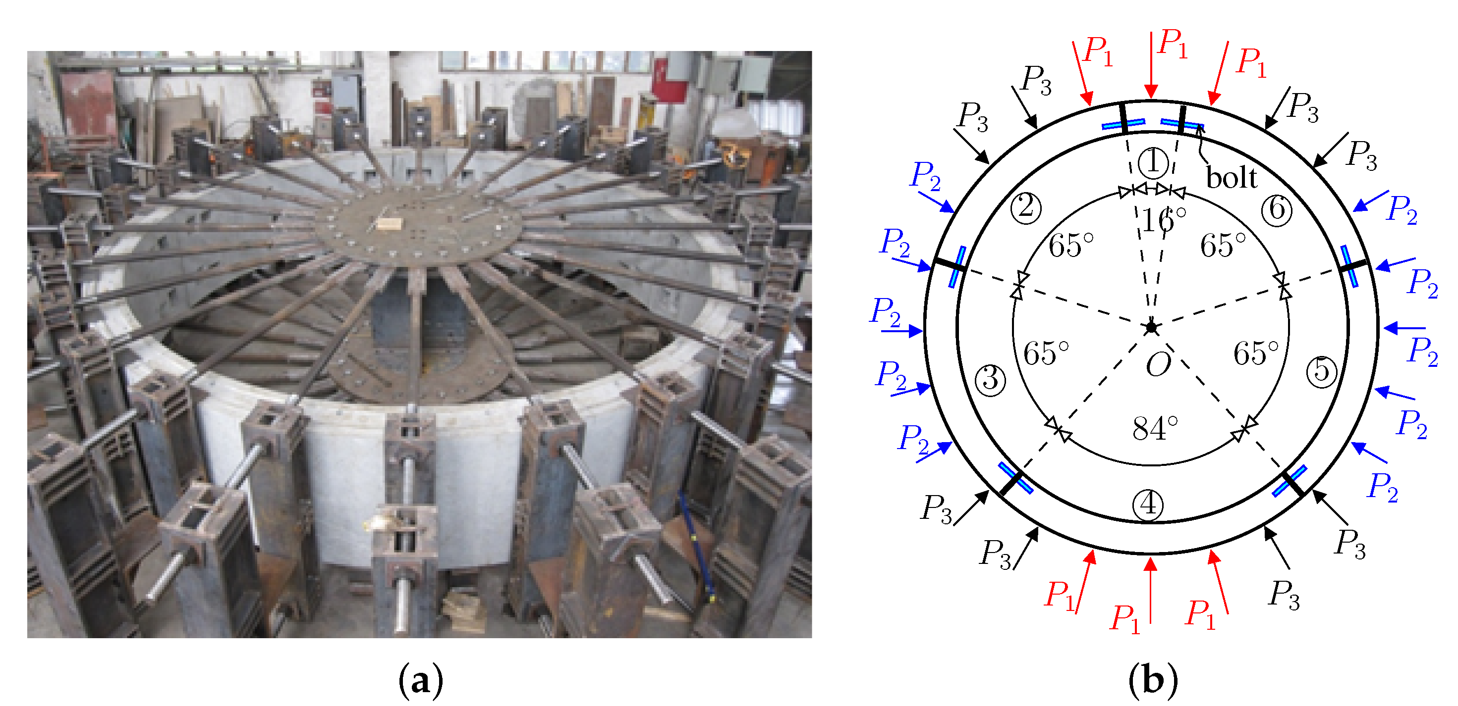
Three real-scale tests, see Figure 1a, are considered in the present paper. The tested rings are symmetrically assembled. They consist of six tubbings; see Figure 1.

Figure 1.
(a) Photo of the testing facility for segmental tunnel linings; (b) symmetric layout and loading of the rings.
The radius of the axes of the rings, R, amounts to , the axial length to , and the radial thickness of the segments, t, to . The bending stiffness, , and extensional stiffness, , of the rings are and , respectively. The segmental joints were positioned at the angular coordinates , , , , , and ; see also Table 2. Bolts connected neighboring tubbings; see Figure 1b and [34] for details.
Table 2.
Geometric and mechanical properties of the tested linings.
The tested structures were loaded by 24 point loads, provided by 24 hydraulic jacks, which were symmetrically deployed. They included six loads , ten loads , and eight loads ; see Figure 1b. Test 1 served as a reference; see [34,35] for the experimental data and structural analysis. Phase 1 of Tests 2 and 3, at least nominally, repetitions of Test 1; see Figure 2a and Figure 3a for the intensities of the point loads. The experimental data of Test 2 have been published [37], while those of Test 3 are first reported in the present paper. The first ten load steps in both tests referred to the application of the design value of the in situ ground pressure. The next load steps simulated the increase in the ground pressure resulting from the overload above the tunnel. The coefficient of lateral ground pressure amounted to , i.e., . is the mean value of and , simulating the ground pressure on the shoulder of the structures. , , and were increased simultaneously until reached the passive ground pressure, which occurred at load step 18 in Test 2. Thereafter, was kept constant. was further increased and was chosen as .

Figure 2.
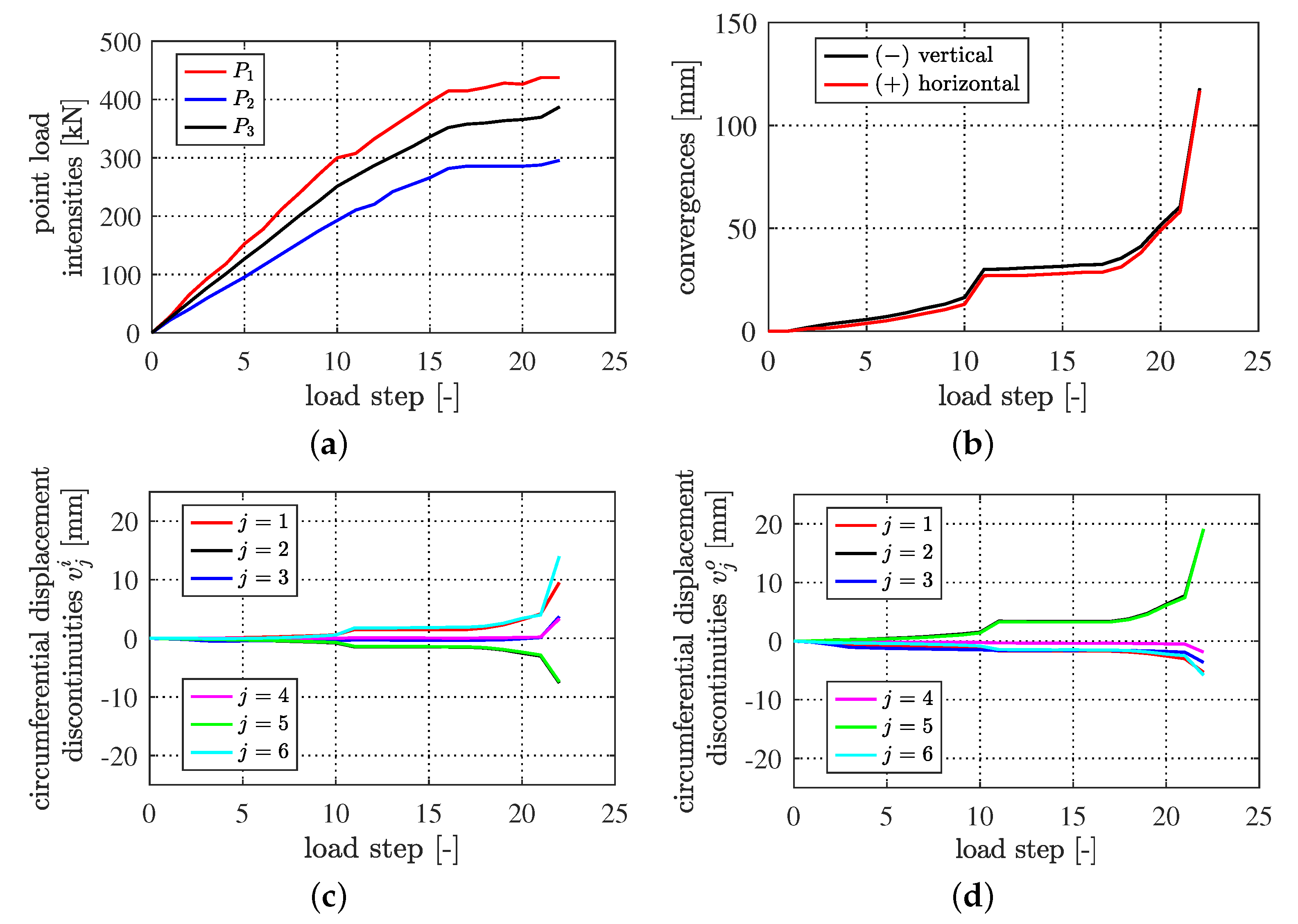
Experimental data of Test 2: (a) intensities of the point loads; (b) measured convergences; (c,d) refer to measured inner and outer circumferential displacements of the joints, respectively.

Figure 3.
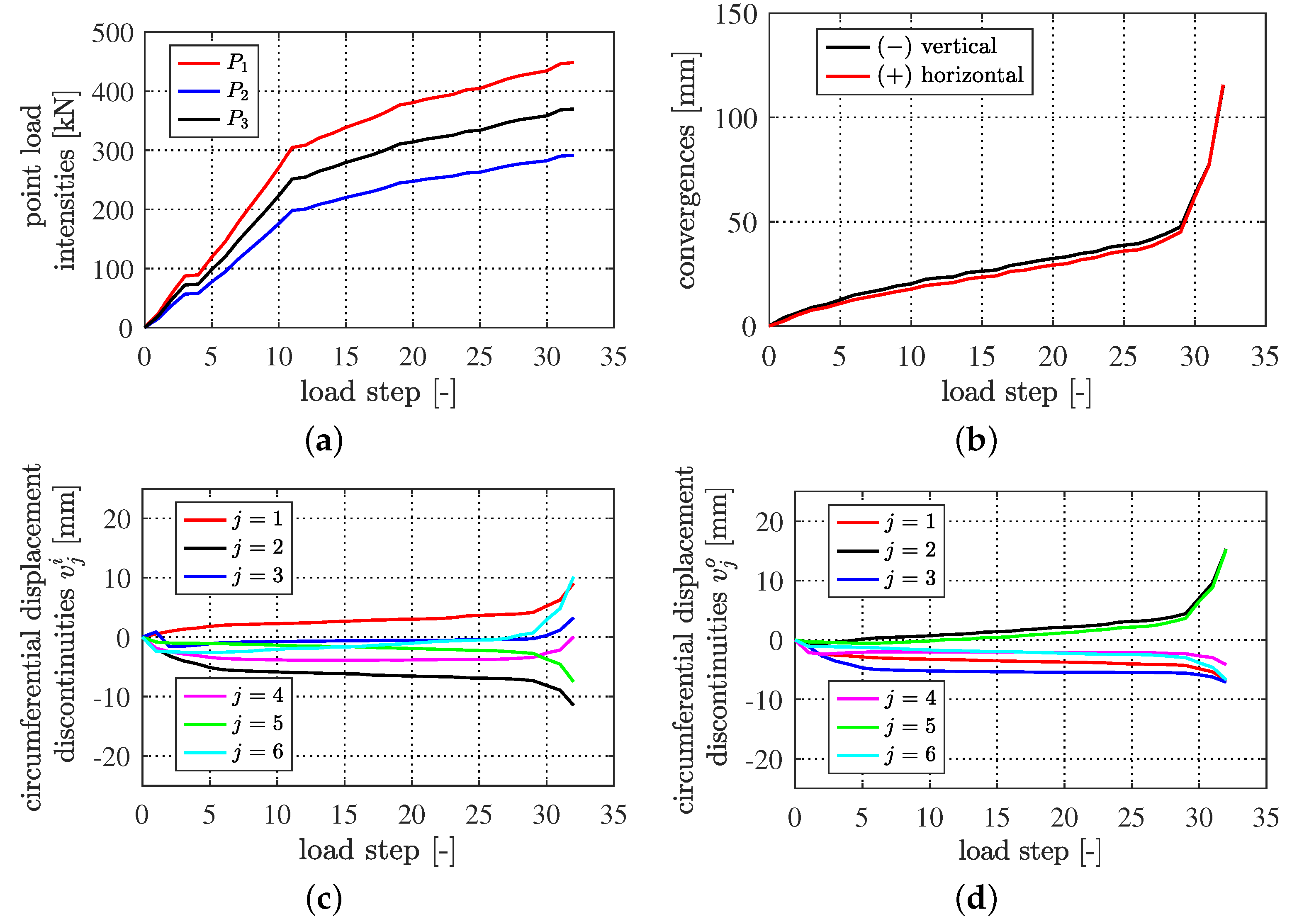
Experimental data of Test 3: (a) intensities of the point loads; (b) measured convergences; (c,d) refer to measured inner and outer circumferential displacements of the joints, respectively.
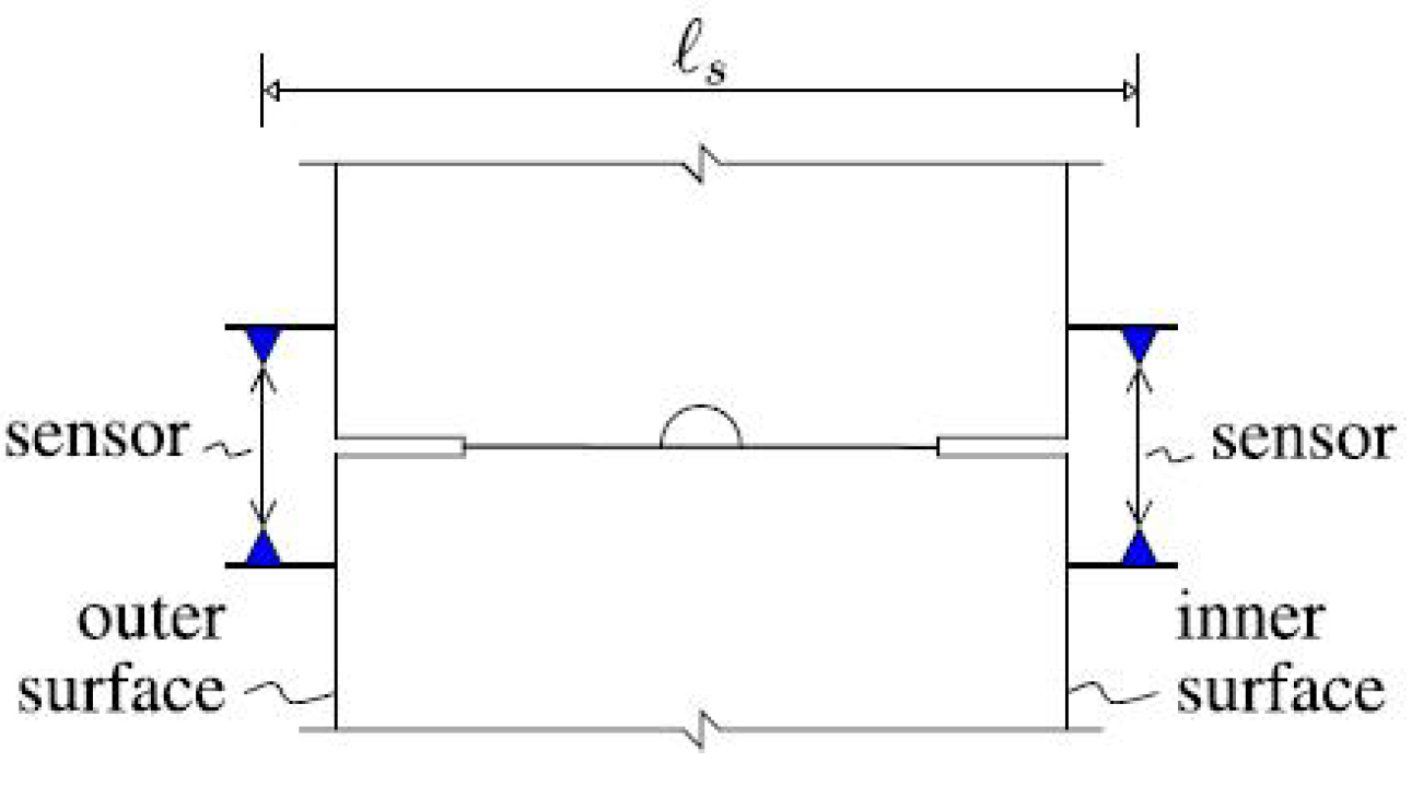
During the test, the circumferential displacements of the inner and outer gaps of the six joints as well as the horizontal and vertical convergences, see Figure 4, were measured. The measured data of Test 1 are shown in Figures 3b, 5, and 6 of [35] and those of Test 2 and Test 3 in Figure 2b–d and Figure 3b–d. and in Figure 2 are the inner and outer circumferential displacements at the jth intersegmental joint, with , respectively. The angular coordinates of the jth joint are shown in Table 2. As described in the Introduction, the convergence-related categorization of the serviceability of the tested tunnel rings, with as the value of the outer diameter , is provided in Table 3. In Test 1, the serviceability was violated because the maximum convergences reached values larger than ; see Figure 6 in [35]. In Tests 2 and 3, the serviceability was endangered because the maximum convergences reached values larger than but smaller than ; see Figure 2b and Figure 3b.

Figure 4.
Positions of the displacement sensors measuring the inner and outer circumferential displacements of the joints [35]; the sensor distances, , amounted to in Test 1 and to in Tests 2 and 3.
Table 3.
Convergence-related serviceability of the tested segmental tunnel linings resulting from use of in Table 1.
3. Hybrid Analysis
3.1. Transfer Relations
Transfer relations, obtained by means of the first-order theory of slender circular arches, are employed for the structural analysis. They read as [34]
where [34]
In Equations (2) and (3), u and v denote the radial and circumferential displacements of the axis of the arch, denotes the rotation of the cross-section, and denotes the circumferential coordinate. Moreover, R, , and stand for the radius of the axis of the arch, the bending stiffness, and the extensional stiffness, respectively. Further, M, N, and V stand for the bending moment, the axial force, and the shear force, respectively. The vector on the left-hand side of Equation (2) refers to the radial and circumferential displacements, the cross-sectional rotation, and the inner forces of the cross-section at an arbitrary value of the angular coordinate . The vector on the right-hand side of Equation (2) contains six integration constants referring to the radial and circumferential displacements, the cross-sectional rotation, and the inner forces of the cross-section at the initial cross-section (index i), i.e., at the circumferential position . The summation symbols in the last column of the transfer matrix in Equation (2) refer to the superposition of so-called load integrals (superscript L). The load integrals for a radial point load, , acting at position , read as [34]
where stands for the Heaviside function. Discontinuities of kinematic variables, occurring at the segmental joints, result in rigid-body displacements. In the mathematical expression for these displacements, the relative rotations of the joints, , located at , , are the governing kinematic variables. However, the influence of the radial and circumferential displacements at the joints, and , respectively, is insignificant. Thus, they can be neglected [35]. The load integrals for read as [34]
The six integration constants at the initial cross-section in Equation (2) are obtained as follows: firstly, the three kinematic integration constants are set equal to zero. Secondly, the computation of the three static integration constants is based on three continuity conditions of a closed ring. They read as [35]
resulting in [34]
where the summation symbols refer to the superposition of the load integrals, evaluated for .
3.2. Strategy for Symmetric Rigid-Body Displacements
Hybrid analysis of a full-scale test of the symmetrically assembled tunnel ring, shown in Figure 1, subjected to symmetric external loadings, was carried out in [34]. Both external loading and measured discontinuities at the segmental joints were employed as input. It was found that the rigid-body displacements of the segments are responsible for 95% of the convergences, while the deformations of the segments resulting from the internal forces contribute to the convergences only by approximately 5%.
The radial displacement of the axis of the tunnel lining at an arbitrary value of the angular coordinate, , denoted as , was calculated as [34]
results from the rigid-body displacements caused by the relative rotations of the joints, , located at with . With respect to symmetric rigid-body displacements, i.e., with , the vertical and horizontal convergences, denoted as and , respectively, are obtained as
The input variables, , are quantified and improved with the help of the strategy for symmetric rigid-body displacements. The Bernoulli–Euler hypothesis (index ) was employed for the first estimates of the relative rotations as the difference of the circumferential displacements, measured at the inner and outer surfaces, , divided by the sensor distance, denoted as , i.e.,
Then, were symmetrized with respect to the vertical axis of the tunnel ring as
This results in the reduction in the number of variables from six to three. Increments are added to to obtain relative rotations referring to rigid-body displacements (index ) as
In order to calculate , the following conditions must be fulfilled: (1) the segmental rings must remain closed rings (continuity conditions), i.e., the displacements at both and must be the same; (2) the discontinuities refer to pure rigid-body displacements that do not generate internal forces in the ring; and (3) the quantities are defined as the minimum of the sum of their squares. Thus, they refer to the smallest improved increments. The solution for reads as [35]
3.3. Symmetric Model of Rigid-Body Displacements
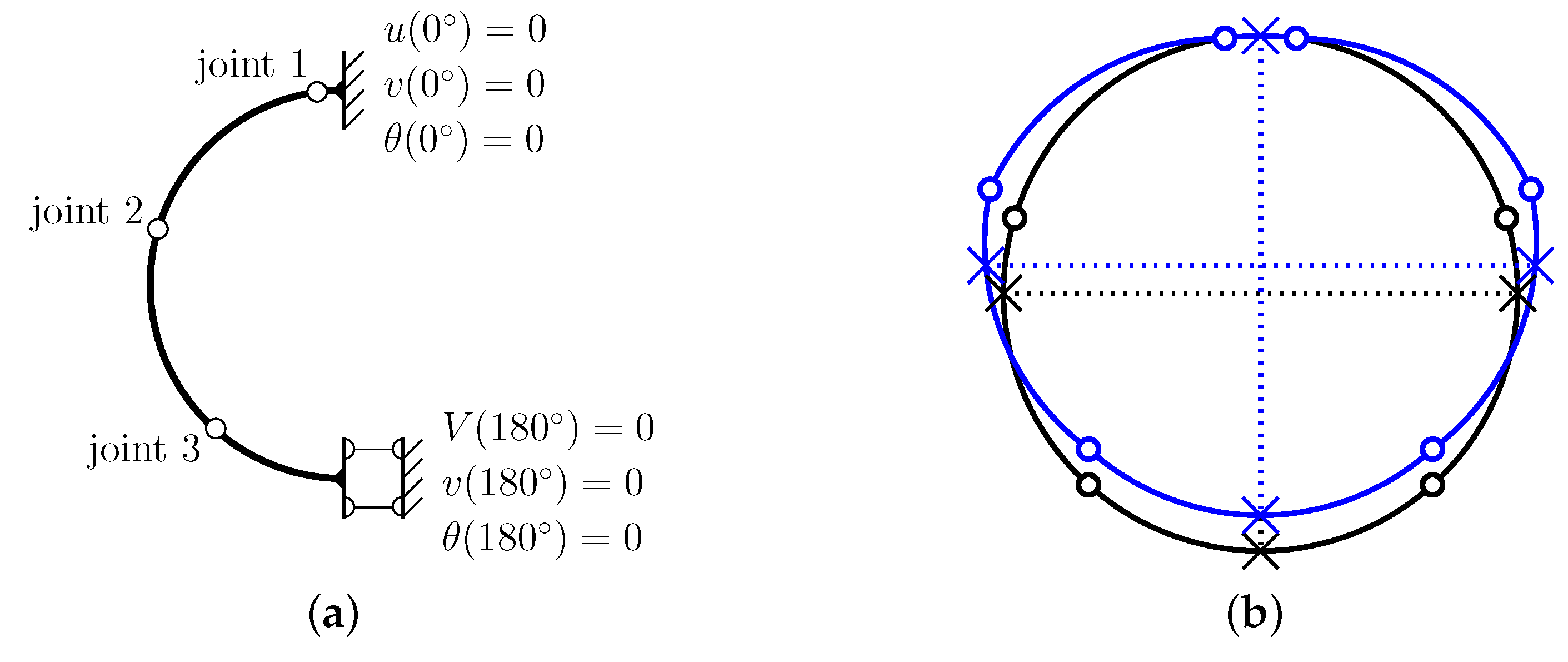
The segmental tunnel linings analyzed in the present paper have six degrees of freedom (DOFs), as shown in Figure 1. Three overall DOFs, i.e., one rotational DOF and two translational DOFs, do not result in convergences because they refer to displacements of the tunnel structure as a rigid body. Three internal DOFs refer to rigid-body displacements of the segments relative to each other. Herein, three overall DOFs are set equal to zero, see in Equation (14). Thus, the remaining types of rigid-body displacements represent quantities relative to the segment at the top, which serves as the reference.
As for the symmetric mode of rigid-body displacements, see Figure 5a for the half-ring model, the values of , referring to rigid-body displacements, must fulfill the following three conditions, expressing that the analyzed rings remain closed [35]:

Figure 5.
Symmetric mode of rigid-body displacements: (a) half-ring models for the analysis and (b) graphical representation.
Symmetric relative rotations, , fulfill the conditions , , and . Inserting them into Equations (30)–(32), it is observed that Equation (30) is automatically satisfied. The reason is that the sine function is asymmetric with respect to the vertical axis, whereas the relative rotations are symmetric. The other two conditions, i.e., (31)–(32), read as
For the purpose of solving these two equations with three unknowns, one of the unknowns must be prescribed. The other two follow in the sense of an inevitable kinematic chain. This provides the motivation to express the angles as functions of , yielding the general solution
The graphical representation of symmetric rigid-body displacements, see Figure 5b, is obtained with the help of the transfer relations (2), where the load integrals for are calculated by inserting Equations (35)–(37) into Equations (10)–(13). The six integration constants at the initial cross-section are set equal to zero because rigid-body displacements do not generate internal forces.
As for the analysis of the rings investigated herein, is inserted into Equations (35)–(37), using the values of from Table 2. The symmetric mode of rigid-body displacements in form of the row vector is obtained as follows:
It is then orthonormalized as
The vertical and horizontal convergences are calculated by superposition of the radial displacements of the top and bottom of the ring and of the ones at the “3 o′clock” and the “9 o′clock” position, respectively, of the symmetric mode of rigid-body displacements, i.e.,
The radial displacements at these positions are calculated with the help of the transfer relations (2). Given that
the expression for the ratio of the vertical and horizontal convergences of the symmetric mode of rigid-body displacements is obtained as
Inserting the values of of the analyzed rings (Table 2) into Equation (43), the value of this ratio is obtained as
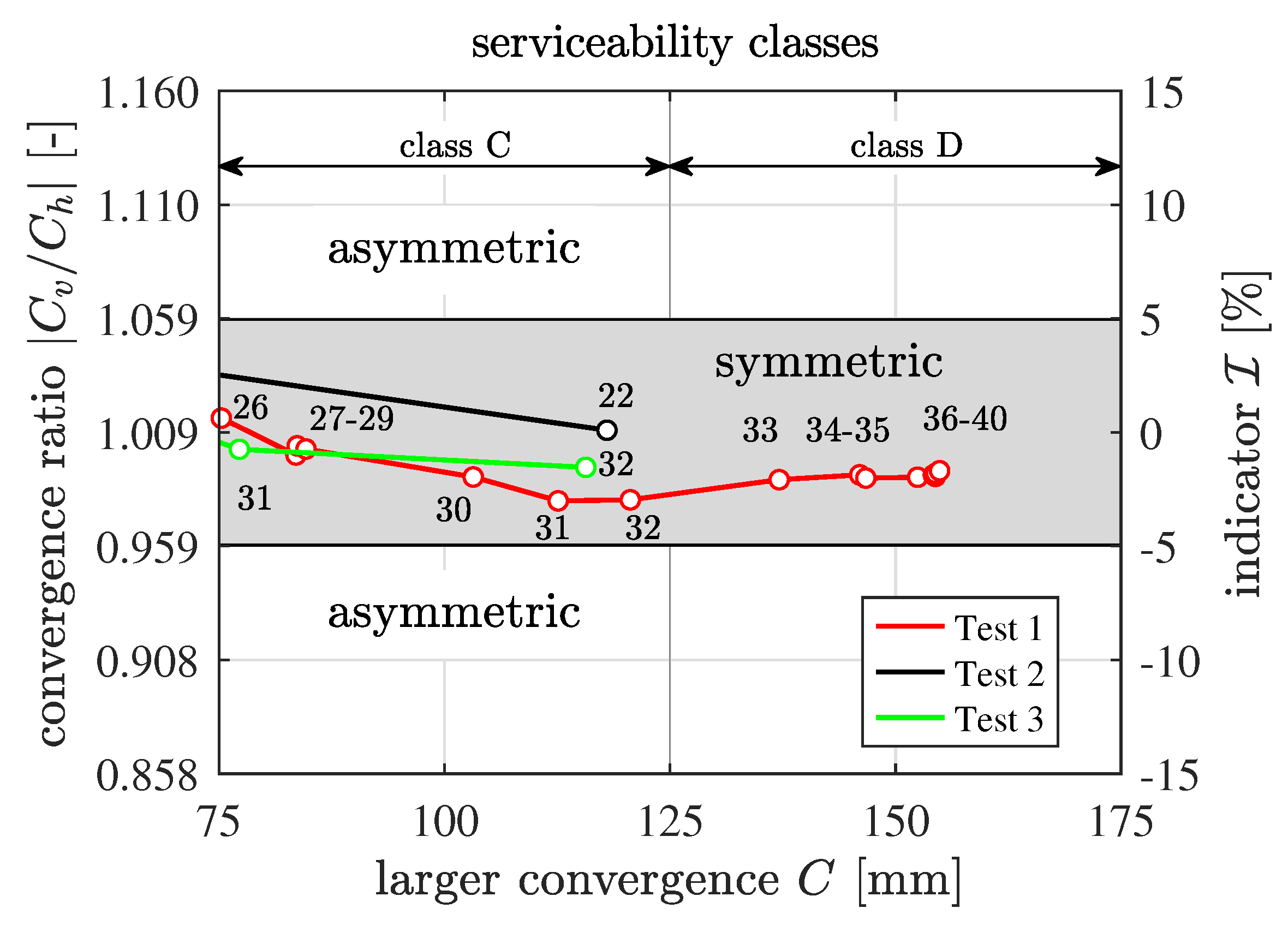
An index was defined to distinguish between the categories of symmetric and asymmetric problems. It reads as [13]
where and are the vertical and horizontal convergences measured in the test, and is the ratio of the vertical and horizontal convergences for the symmetric mode of rigid-body displacements. If is larger than , the test is considered to represent an asymmetric problem [13]. The development of for the three tests analyzed in this paper is shown in Figure 6 as functions of C. The range of the abscissa is limited to convergences for which the serviceability is endangered. Because the values of of all three tests are smaller than , these tests fall into the category of symmetric problems.

Figure 6.
Categorization of real-scale tests of segmental tunnel linings as symmetric and asymmetric problems, respectively, based on the index ; the abscissa is limited to convergences that are so large that the serviceability is endangered; see Table 3.
4. Extended Hybrid Method
4.1. Application of the Hybrid Method Using the Strategy of Symmetric Rigid-Body Displacements
As described in Section 3.2, for symmetric problems, the covergences are linear functions of the radial displacements. This enables subdividing the calculation into two load cases. Load case I refers to point loads, while the relative rotations are set equal to zero. It was found that of the convergences result from load case II [35].
As for load case II, the input variables, , are quantified and improved by the strategy of symmetric rigid-body displacements. The Bernoulli–Euler hypothesis (index ) was employed for computation of first estimates of the relative rotations as the difference in the circumferential displacement jumps, measured at the inner and the outer surfaces, , divided by the sensor distance ; see Equation (24). Then, the quantities are symmetrized with respect to the vertical axis of the ring; see Equation (25). The increments are added to to obtain relative rotations referring to rigid-body displacements (index ); see Equation (26). The quantities are calculated by inserting Equation (26) into the conditions (30)–(32). With the help of the additional condition
involving the smallest improved increments, is computed. The overall displacements are calculated by superposition of the displacements obtained from load case I and load case II. In load case I, the convergences are calculated with the help of the transfer relations (2). Point load intensities, recorded during testing, are inserted into Equations (4)–(9) as the load integrals of the external loading. The load integrals of the relative rotations are set equal to zero. , , and follow from Equation (14). , , and are obtained from Equations (18)–(20). In load case II, the convergences are calculated with the help of the transfer relations (2), where the load integrals of the external loading are set equal to zero. The load integrals of the relative rotations are obtained by inserting the relative rotations into Equations (11)–(13). , , , , , and are set equal to zero.
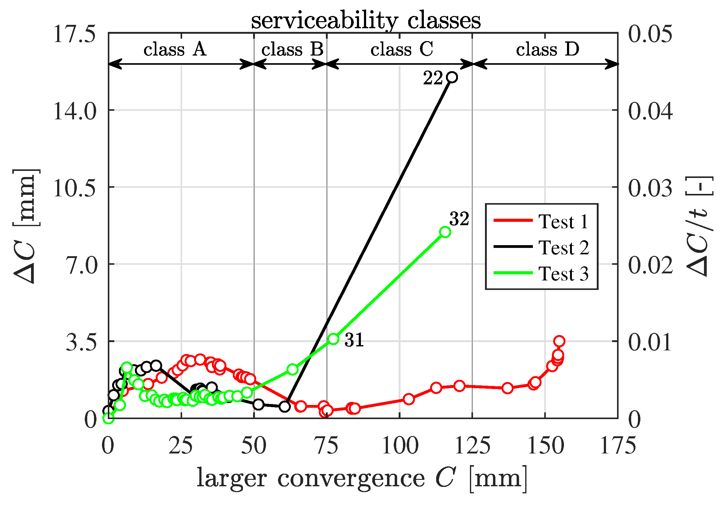
The above-described method was applied to the three tests. The error of the simulation is defined as
where
and denote the vertical and horizontal convergences, respectively, obtained from the model simulation. Dividing by the thickness of the segments, t, a dimensionless index is obtained as
and are shown in Figure 7 as functions of the larger convergence, C. The following categorization is proposed. Provided that the error index is smaller than or equal to , the accuracy is acceptable. If the error index is larger than , the accuracy is not acceptable. It is shown that the structural displacements in Test 1 are reproduced with high accuracy during the whole loading process. However, the structural displacements in Tests 2 and 3 are not reproduced accurately when the structure enters into serviceability class C. Hence, an improved strategy of symmetric rigid-body displacements is needed.

Figure 7.
Error indices—larger convergence C diagrams using the strategy of symmetric rigid-body displacements proposed by [35].
4.2. Improved Strategy of Symmetric Rigid-Body Displacements
In Figure 7, it is shown that the convergences in Test 2 after load step 21 and in Test 3 after load step 30 are not reproduced by the strategy of symmetric rigid-body displacements. Inaccuracies occur when the structures reach convergence-related serviceability class C. Hence, an improved strategy is needed. Additional symmetric rigid-body displacements are added such that the measured convergences are reproduced. The improved strategy of rigid-body displacements is described in the following. At first, are calculated by means of the strategy of symmetric rigid-body displacements. Then, additional relative rotations are added to , resulting in
where denotes the orthonormalized vector of the relative rotations in the symmetric mode of rigid-body displacements. The vertical and horizontal convergences from the model simulation are expressed as
because they are linear functions of the relative rotations in case of the mode of symmetric rigid-body displacements. In Equations (52) and (53), and are the vertical and horizontal convergences resulting from . and are calculated by inserting Equation (39) into the transfer relations (2). They read as
Hence, and are the functions of the unknown . To obtain the smallest error index, is calculated by the condition
It is obtained as
4.3. Presentation and Discussion of Results
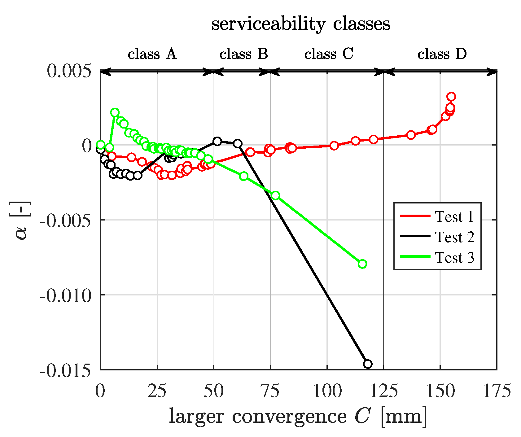
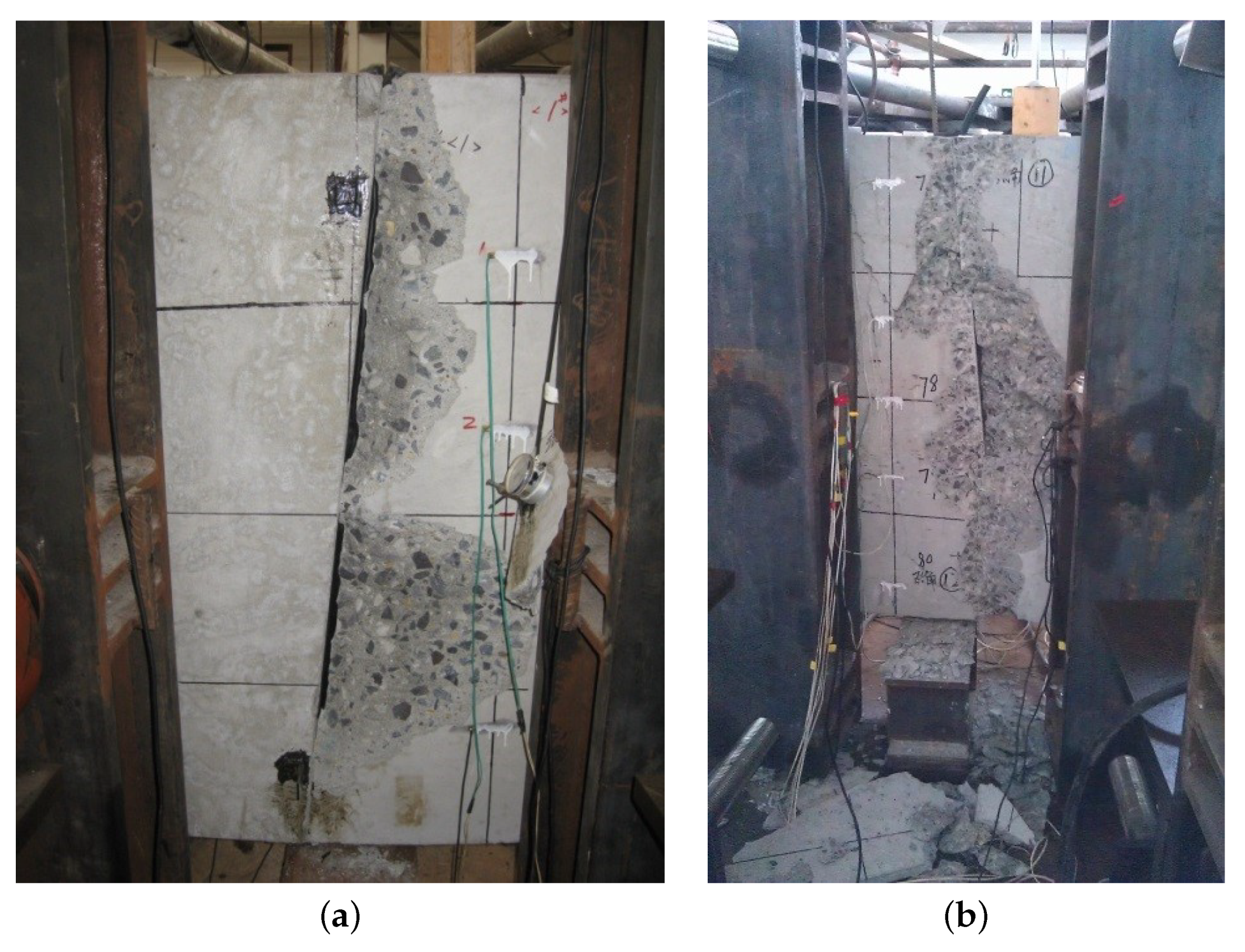
The improved strategy of symmetric rigid-body displacements was applied to Tests 1, 2, and 3 from the beginning of the loading process. The development of , as the larger convergence C increases, is shown in Figure 8. For Test 1, is small, and it changes only mildly during the loading process. This underlines that realistic relative rotations of the joints are obtained by means of combining the measured circumferential displacement jumps at the inner and outer surfaces of the joints with the Bernoulli–Euler hypothesis, followed by symmetrization. The deformed structural configuration is reproduced with high accuracy. However, for Tests 2 and 3, increases strongly when the larger convergences exceed 75mm (serviceability class C). This implies that, for Tests 2 and 3, extra rigid-body displacements are required in order to reproduce the measured convergences once the structure enters serviceability class C. The reason for this situation is that sudden failure, such as spalling of concrete, occurred in the vicinity of the segmental interfaces when the structures were close to SLS. This resulted in movements of the displacement sensors deployed on the surfaces of the interfaces. This leads to inaccuracies in the measured data in the tests at the last load steps. Such failure was observed in the tests. As shown in Figure 9, the outer concrete spalled at joint 1 at load level 22 in Test 2 and at joint 6 at load level 31 in Test 3. Hence, in such situations, additional data, i.e., measured convergence, are employed to reproduce the accurate deformed structural configuration. Different from the asymmetric problem, where the asymmetric structural behavior develops in a progressive and subtle fashion [13], for the third class of problems, this behavior develops in a sudden fashion.

Figure 8.
—larger convergence C diagrams using the improved strategy of symmetric rigid-body displacements.

Figure 9.
Concrete spalling at the outer surface: (a) at segmental joint 1 at load level 22 in Test 2 and (b) at segmental joint 6 at load level 31 in Test 3.
In practical applications, the outer surface is inaccessible. Thus, the cracking and spalling of the concrete at the outer surface remain unnoticed. If the tunnel is in an aggressive environment, with a particular risk of corrosion of the reinforcement of the segments, cracking at the outer surface is not acceptable. In such a case, it is better to reduce to , used herein and in [13]. Otherwise, is sufficient.
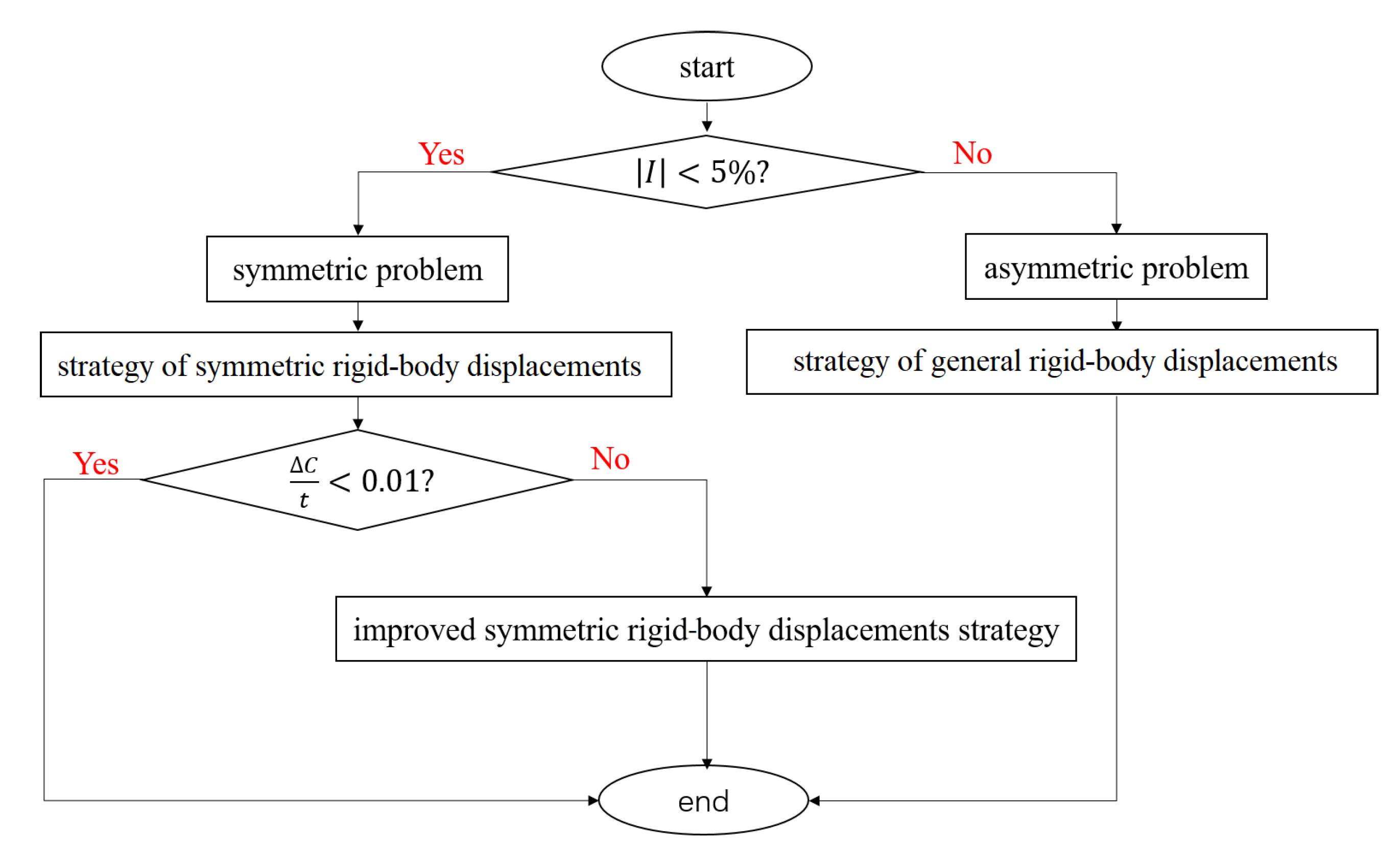
To reproduce the deformed structural configurations, the following procedure is proposed. As shown in Figure 10, at first, the symmetry indicator is calculated with the help of the measured vertical and horizontal convergences to categorize the problem as symmetric or asymmetric. As for the latter, the strategy of general rigid-body displacements is to be employed. For symmetric problems, the strategy of symmetric rigid-body displacements is to be used. The accuracy of the simulation is checked by the error index . If this index is smaller than , the calculation is finished. However, if it is larger than , the here-proposed strategy of symmetric rigid-body displacements should be employed.

Figure 10.
Decision tree of structural analysis of segmental tunnel linings.
5. Conclusions
- The structural analysis of segmental tunnel rings can be categorized into only three classes: Class A is the category of asymmetric problems [13]. Class B includes symmetric problems without sudden failures at the joints during the loading process [35], and Class C is the category of symmetric problems with some sudden failures, such as concrete spalling, at the segmental interfaces.
- An efficient analysis procedure was proposed in this paper. With the help of , the analysis problem was, at first, categorized as an asymmetric or a symmetric problem. For the asymmetric problems, the strategy of general rigid-body displacements was employed. For the symmetric problems, the strategy of symmetric rigid-body displacements was used. The accuracy of the simulations of the symmetric problems was checked by . If it was found to be unacceptable, the improved strategy of symmetric rigid-body displacements was used.
- The reason for the difference between Class A and Class B is different from the reason for the treatment as an asymmetric problem, characterized by the development of the asymmetric structural behavior in a progressive and subtle fashion [13]. The third class of problems is characterized by the development of the deformations in a sudden fashion.
- When convergence-related serviceability class C is reached, the stress state or the failure states of the interfaces need to be checked carefully. Local failure results in a rapid increase in structural deformations. Serviceability class D will then be reached soon.
- It is suggested that, upon the attainment of convergence-related serviceability class C and the detection of local failure at segmental interfaces, the strengthening of the structure should be considered at serviceability class C rather than only at serviceability class D, i.e., at the SLS.
- If the tunnel is located in an aggressive environment and the cracking at the outer surface is not acceptable, the definition of the convergence-related SLS should be stricter. In this case, should be set equal to rather than to .
- The accuracy of the extended hybrid method was validated by means of monitoring the data collected during full-scale testing. In the future, it will be interesting to equip real tunnels with advanced monitoring techniques that enable the collection of similar data, and to use these data for the further validation of the applicability of the method presented.
Author Contributions
Conceptualization, B.P. and Z.J.; methodology, Z.J. and J.Z.; software, Z.J.; validation, Z.J. and B.P.; formal analysis, Z.J.; investigation, Z.J.; resources, Z.J. and X.L.; data curation, Z.J. and X.L.; writing—original draft preparation, Z.J.; writing—review and editing, H.A.M.; supervision, B.P. and H.A.M. All authors have read and agreed to the published version of the manuscript.
Funding
Financial support by China Scholarship Council (CSC) to the first author.
Data Availability Statement
Data is contained within the article.
Acknowledgments
Financial support of the first author by the China Scholarship Council (CSC) is gratefully acknowledged. Open Access Funding by TU Wien.
Conflicts of Interest
The authors declare no conflicts of interest.
References
- Chang, C.T.; Sun, C.W.; Duann, S.W.; Hwang, R.N. Response of a Taipei Rapid Transit System (TRTS) tunnel to adjacent excavation. Tunn. Undergr. Space Technol. 2001, 16, 151–158. [Google Scholar] [CrossRef]
- Avanaki, M.J. Effects of hybrid steel fiber reinforced composites on structural performance of segmental linings subjected to TBM jacks. Struct. Concr. 2019, 6, 1909–1925. [Google Scholar] [CrossRef]
- Li, X.; Lin, X.; Zhu, H.; Wang, X.; Liu, Z. Condition assessment of shield tunnel using a new indicator: The tunnel serviceability index. Tunn. Undergr. Space Technol. 2017, 67, 98–106. [Google Scholar] [CrossRef]
- Sun, W.; Han, F.; Zhang, Y.; Zhang, W.; Zhang, R.; Su, W. Experimental assessment of structural responses of tunnels under the groundwater level fluctuation. Tunn. Undergr. Space Technol. 2023, 137, 105138–105153. [Google Scholar] [CrossRef]
- Gong, W.; Juang, C.H.; Huang, H.; Zhang, J.; Luo, Z. Improved analytical model for circumferential behavior of jointed shield tunnels considering the longitudinal differential settlement. Tunn. Undergr. Space Technol. 2015, 45, 153–165. [Google Scholar] [CrossRef]
- British Tunnelling Society. Tunnel Lining Design Guide; Thomas Telford: London, UK, 2004. [Google Scholar]
- German Tunnelling Committee. Recommendations for the Design, Production and Installation of Segmental Rings; German Tunnelling Committee: Cologne, Germany, 2013. [Google Scholar]
- GB50157; Code for Design of Metro. Ministry of Housing and Urban-Rural Development of the People’s Republic of China: Beijing, China, 2013.
- DGJ08-11-99; Shanghai Foundation Design Code. Shanghai Construction Committee: Shanghai, China, 1999.
- Peck, R. Deep excavations and tunneling in soft ground. In Proceedings of the 7th International Conference on Soil Mechanics and Foundation Engineering, Mexico City, Mexico, August 1969. [Google Scholar]
- Carpio, F.; Peña, F.; Galván, A. Recommended deformation limits for the structural design of segmental tunnels built in soft soil. Tunn. Undergr. Space Technol. 2019, 90, 264–276. [Google Scholar] [CrossRef]
- DG/TJ08-2123-2013; Code for Structural Appraisal of Shield Tunnel. Shanghai Municipal Commission of City Development and Transport: Shanghai, China, 2013.
- Jiang, Z.; Liu, X.; Schlappal, T.; Zhang, J.; Mang, H.A.; Pichler, B.L. Asymmetric serviceability limit states of symmetrically loaded segmental tunnel rings: Hybrid analysis of real-scale tests. Tunn. Undergr. Space Technol. 2021, 113, 103832. [Google Scholar] [CrossRef]
- Chang, C.T.; Wang, M.J.; Chang, C.T. Repair of displaced shield tunnel of the Taipei rapid transit system. Tunn. Undergr. Space Technol. 2001, 15, 167–173. [Google Scholar] [CrossRef]
- Kiriyama, K.; Kakizaki, M.; Takabayashi, T.; Hirosawa, N.; Takeuchi, T.; Hajohta, H. Structure and construction examples of tunnel reinforcement method using thin steel panels. Nippon. Steel Tech. Rep. 2005, 92, 45–50. [Google Scholar]
- Gu, C. Structural reinforcement technology for deformed tunnels. Shield Tunn. Technol. 2013, 1, 21–25. [Google Scholar]
- Moss, N. London underground monitoring: Recent experience and future requirements. In Proceedings of the First International Workshop on Monitoring and Inspection of Metro Tunnel, Tongji University, Shanghai, China, 26–28 May 2014. [Google Scholar]
- Kontogianni, V.; Stiros, S. Tunnel deformation during excavation—A kinematic approach based on geodetic observations. Field Meas. Geomech. 2003, 1, 189–193. [Google Scholar]
- Kontogianni, V.; Stiros, S. Induced deformation during tunnel excavation: Evidence from geodetic monitoring. Eng. Geol. 2005, 79, 115–126. [Google Scholar] [CrossRef]
- Barla, G.B.; Bonini, M.; Debernardi, D. Time dependent deformations in squeezing tunnels. In Proceedings of the 12th International Conference of International Association for Computer Methods and Advances in Geomechanics, Goa, India, 1–6 October 2008. [Google Scholar]
- Stiros, S.; Kontogianni, V. Mean deformation tensor and mean deformation ellipse of an excavated tunnel section. Int. J. Rock Mech. Min. Sci. 2009, 46, 1306–1314. [Google Scholar] [CrossRef]
- Nakai, T.; Maruki, Y.; Ryu, M.; Ohnishi, Y.; Nishiyama, S.; Tatebe, T.; Komae, M. Support design of river crossing tunnel using keyblock concept and its validation by monitoring of the countermeasure by digital photogrammetry. Tunn. Undergr. Space Technol. 2004, 19, 440–441. [Google Scholar]
- Hashimoto, T.; Koyama, Y.; Yingyongrattanakul, N.; Kayukawa, K.; Sugimoto, M. Applications of the New Deformation Meter for Monitoring Tunnel Lining Deformation. In Proceedings of the International Symposium on Underground Excavation and Tunnelling, Bangkok, Thailand, 15–16 May 2006. [Google Scholar]
- Yu, Q.; Jiang, G.; Chao, Z.; Fu, S.; Shang, Y.; Yang, X. Deformation monitoring system of tunnel rocks with innovative broken-ray videometrics. In Proceedings of the ICEM: International Conference on Experimental Mechanics, Nanjing, China, 8–12 November 2008. [Google Scholar]
- Kavvadas, M. Monitoring ground deformation in tunnelling: Current practice in transportation tunnels. Eng. Geol. 2005, 79, 93–113. [Google Scholar] [CrossRef]
- Shan, J.; Toth, C.K. Topographic Laser Ranging and Scanning: Principles and Processing. In Scanning Principles and Processing; CRS Press: Boca Raton, FL, USA, 2014; pp. 215–234. [Google Scholar]
- Gosliga, R.V.; Lindenbergh, R.; Pfeifer, N. Deformation analysis of a bored tunnel by means of terrestrial laser scanning. Image Eng. Vis. Metrol. ISPRS Comm. 2006, 36, 167–172. [Google Scholar]
- Jaboyedoff, M.; Demers, D.; Locat, J.; Locat, A.; Turmel, D. Use of terrestrial laser scanning for the characterization of retrogressive landslides in sensitive clay and rotational landslides in river banks. Rev. Can. Gotechnique 2009, 46, 1379–1390. [Google Scholar] [CrossRef]
- Nguyen, H.T.; Fernandez-Steeger, T.M.; Wiatr, T.; Rodrigues, D.; Azzam, R. Use of terrestrial laser scanning for engineering geological applications on volcanic rock slopes—An example from Madeira island (Portugal). Nat. Hazards Earth Syst. Sci. 2011, 11, 807–817. [Google Scholar] [CrossRef]
- Abellan, A.; Vilaplana, J.M.; Calvet, J.; García-Sellés, D.; Asensio, E. Rockfall monitoring by Terrestrial Laser Scanning—Case study of the basaltic rock face at Castellfollit de la Roca (Catalonia, Spain). Nat. Hazards Earth Syst. Sci. 2011, 11, 829–841. [Google Scholar] [CrossRef]
- Granitzer, A.N.; Tschuchnigg, F. Numerical Analysis of Segmental Tunnel Linings employing a Hybrid Modeling Approach. Comput. Eng. Phys. Model. 2021, 4, 1–18. [Google Scholar]
- Sun, W.; Zhang, W.; Goh, A.T.C.; Zhang, R. Experimental and computational analysis of hydraulic behavior in shallow buried structures in sand. Gondwana Res. 2023, 124, 339–350. [Google Scholar] [CrossRef]
- Zhang, Y.; Karlovek, J.; Liu, X. Identification method for internal forces of segmental tunnel linings via the combination of laser scanning and hybrid structural analysis. Sensors 2022, 22, 2421. [Google Scholar] [CrossRef] [PubMed]
- Zhang, J.L.; Vida, C.; Yuan, Y.; Hellmich, C.; Mang, H.A.; Pichler, B. A hybrid analysis method for displacement-monitored segmented circular tunnel rings. Eng. Struct. 2017, 148, 839–856. [Google Scholar] [CrossRef]
- Zhang, J.L.; Mang, H.A.; Liu, X.; Yuan, Y.; Pichler, B. On a nonlinear hybrid method for multiscale analysis of a bearing capacity test on a real-scale segmental tunnel ring. Int. J. Numer. Anal. Methods Geomech. 2019, 43, 1343–1372. [Google Scholar] [CrossRef] [PubMed]
- Liu, X.; Bai, Y.; Yuan, Y.; Mang, H.A. Experimental investigation of the ultimate bearing capacity of continuously jointed segmental tunnel linings. Struct. Infrastruct. Eng. 2016, 12, 1364–1379. [Google Scholar] [CrossRef]
- Liu, X.; Jiang, Z.; Yuan, Y.; Mang, H.A. Experimental investigation of the ultimate bearing capacity of deformed segmental tunnel linings strengthened by epoxy-bonded steel plates. Struct. Infrastruct. Eng. 2018, 14, 685–700. [Google Scholar] [CrossRef]
Disclaimer/Publisher’s Note: The statements, opinions and data contained in all publications are solely those of the individual author(s) and contributor(s) and not of MDPI and/or the editor(s). MDPI and/or the editor(s) disclaim responsibility for any injury to people or property resulting from any ideas, methods, instructions or products referred to in the content. |
© 2024 by the authors. Licensee MDPI, Basel, Switzerland. This article is an open access article distributed under the terms and conditions of the Creative Commons Attribution (CC BY) license (https://creativecommons.org/licenses/by/4.0/).