Abstract
Following the Belt and Road, the Air Silk Road has also been proposed. The coordinated development of multiple transportation modes, including air, land, and water, will create a strong transportation force in node cities. However, the current insufficient supply of cargo in various regions and the lack of integration among different transportation modes result in low transportation efficiency, which in turn affects the further advancement of the Belt and Road. To investigate these issues and attempt to find a solution, we selected 44 candidate cities from the prefecture-level cities in China as nodes based on relevant government policies, and constructed an integrated transportation network. For each node city, we first calculated the values of six classical indicators and then used the CRITIC to assign weights to each indicator. Subsequently, we employed the TOPSIS method combined with Grey Relational Analysis (GRA) to compute the comprehensive score for each node city. Based on the spatial layout and government policies under the BRI, eight cities, including Wuhan, Chongqing, Tianjin, Shanghai, Guangzhou, Lianyungang, Hefei, and Dalian, were finally recommended as the consolidation centers of the integrated transportation network. It is hoped that the results of this analysis can provide some insights for the government to outline and build the consolidation centers of the integrated transportation network composed of railway, air, highway, and water routes, which in turn can offer insights for elevating the Belt and Road Initiative (BRI) to a new level.
1. Introduction
The cooperative initiative of establishing the Belt and Road was proposed by Xi Jinping, President of the People’s Republic of China, in Kazakhstan and Indonesia in 2013, respectively, which aims to establish the world’s biggest economic cooperation platform covering Asia, Europe, and sub-regions of Africa and enhance the interconnectivity among countries. Currently, China Railway Express (CR Express), with active participation from local governments, has connected 108 Chinese cities and reached 208 cities in 25 European countries through ports such as Manzhouli, Erenhot, and Alashankou [1]. Meanwhile, as of September 2022, there are 94 routes along Maritime Silk Road, connecting 108 ports in 31 countries [2]. The in-depth development of the transportation network has greatly shortened the time and space distance between China and Europe. Currently, the Chinese local governments are faced with various issues in the process of promoting the in-depth development of the BRI, such as uneven supplies of goods, disordered competition, and inefficient coordination mechanism [3,4]. On the other hand, the Chinese domestic transportation network is a relatively independent development of various transportation modes, which lacks global optimization and integration of transportation resources. To address the above-mentioned issues, constructing consolidation centers through top-level government design is a promising solution to provide rational cargo allocation. This is because the rational location and layout of the consolidation centers can reduce logistics costs through economies of scale, as well as maximize service quality and transportation efficiency within multimodal networks [5,6].
Therefore, the issue of transportation hubs along the Belt and Road has been discussed by many scholars from different perspectives in the past few years. Zhang et al. applied the TOPSIS to sort out the logistics nodes and select the optimal nodes of CR Express under the BRI [7]. Li et al. applied contest theory to validate the number of multimodal transportation network hubs based on local government subsidies under the BRI [8]. Wan et al. used the TOPSIS to identify essential ports in the maritime silk network when encountering severe disasters [9]. By analyzing the quantitative and qualitative factors influencing the location of global logistics centers in the existing literature, Lee et al. proposed the eight locations of global LDCs [10]. Li et al. considered the government policies and operational experience from the BRI, and used the improved entropy TOPSIS to select imported grain distribution centers across railway, highway, and water transportation networks [11]. The TOPSIS was employed by Aljohani et al. to conduct an assessment and ranking of 20 candidate consolidation centers within the city of inner Melbourne, Australia, based on 11 decision criteria, and found that the most suitable locations for the consolidation centers are in economically viable industrial areas [12]. Muerza et al. used ANP technology to evaluate and rank five locations in Europe for establishing international consolidation centers based on 25 standards to support the choices of decision makers [13].
Furthermore, during a meeting with the leader of Luxembourg in June 2017, President Xi Jinping first proposed to build the Air Silk Road between Zhengzhou and Luxembourg. With the gradual integration of the civil aviation industry into the BRI, the Chinese government released an Implementation Plan of the Air Silk Road in May 2022, aiming to promote its in-depth development [14]. Meanwhile, scholars have begun to address the issues of the air transportation network. Zhou et al. employed local centrality and global centrality to research the hub problem of the integration of rail ports, airports, and maritime ports in the Belt and Road countries [15]. Derudder et al. applied the centrality indicator to study the ranking of connectivity of three-layer transportation network node cities for air and highway routes along the Belt and Road [16].
However, the above-mentioned scholars are only concerned about a single mode or a combination of two or three transport modes, and there is less research on the integration of railway, air, highway, and water transportation. Additionally, the whole layout of the integrated transportation network has not been formed at the national level, which cannot effectively fit in with the development of the BRI, making it difficult to effectively achieve the orderly linking up of the multi-tiered integrated transportation network consisting of water, land, and air transportation. Hence, this paper addresses the ranking and selection of node cities as the candidate consolidation centers of an integrated transportation network composed of highway, railway, air, and water routes under the BRI to provide a reference for the government in building the consolidation centers.
A total of 44 Chinese cities were selected as the candidate consolidation centers under the BRI. Then, the integrated transportation network was formed based on the links of transportation modes among these 44 Chinese cities. It should be noted that the evaluation of consolidation centers in this study was based on the consideration of the above issues of cargo transportation at the national level of China under the BRI. Consequently, each city was viewed as a node in the network without delving into the specific logistic activities within it.
Complex network theory has been widely employed in transportation network research in recent years [17,18]; extensive study has been implemented on single-mode transportation networks, including railway networks [11], subway networks [19,20], bus networks [21,22], water networks [23,24], road networks [25], and air networks [26]. Currently, complex network theory is employed by some scholars to study the single-mode transportation networks under the BRI. Zhao et al. used the TOPSIS method combined with complex network theory to select 10 cities from 27 candidate cities as consolidation centers of CR Express [27]. Sun et al. applied the TOPSIS method to select 10 cities from 48 candidate cities of CR Express as consolidation centers using some qualitative indicators [28]. Feng et al. applied the improved TOPSIS method to select the key node of CR Express through multiple centrality evaluation indicators [29]. The entropy weight TOPSIS method was used by Yin et al. [30] to choose eight inner cities as trans-shipment consolidation centers from the regional integration standpoint. Additionally, there are some studies on the impact of consolidation centers. Van Heeswijk et al. applied agent-based data simulation to verify that the urban consolidation center in Copenhagen can reduce truck mileage by about 65% and emissions by about 70% [31]. On the one hand, there is a lack of studies on the integration of various modes such as air, water, railway, and highway transportation in the aforementioned research. On the other hand, the multi-attribute indicators of transportation networks are rarely considered, which makes it difficult to comprehensively evaluate consolidation centers. Consequently, this study employed complex network theory to integrate various transportation modes—including air, water, highway, and railway—with the aim of constructing an integrated transportation network aligned with the BRI. Using this network, we evaluated the comprehensive scores of candidate node cities as potential consolidation centers.
The TOPSIS is a traditional multi-attribute decision-making approach. However, the TOPSIS cannot accurately reflect the similarity of data curves, making it difficult to accurately assess the optimal results. In this study, the TOPSIS combined with Grey Relational Analysis (GRA) was applied, which not only retains the objective advantage of the TOPSIS method but also takes the advantages of the similarity and dynamicity of GRA to make up for the shortcoming of the TOPSIS method. Finally, the ranking results of the candidate consolidation centers are obtained based on the combination of the TOPSIS and GRA.
This paper makes the following contributions. Firstly, the consolidation centers of an integrated transportation network, which includes highway, railway, air, and water routes, is considered as the research target under the BRI to attempt to solve the high logistics costs resulting from disorderly competition, poor efficiency, and so on among the different transportation modes. Secondly, considering the links among the candidate consolidation centers, the TOPSIS and GRA are combined to comprehensively evaluate the ranking of candidate consolidation centers within the integrated transportation network constructed based on complex network theory. Thirdly, the local and global evaluation indicators were integrated to evaluate the candidate consolidation centers of the integrated transportation network.
The remaining sections are as follows: Section 2 introduces the criteria and the steps for selecting node cities. Section 3 establishes transportation networks of air, water, railway, and highway routes. The related evaluation indicators are selected in Section 4. The related approach is depicted in Section 5. A case application is analyzed in Section 6. Section 7 implements a comparative analysis. Finally, Section 8 is the conclusions.
2. Criteria and Procedure for Selecting Consolidation Centers
2.1. Screening Criteria
The Chinese government has issued various documents with regard to the layout of Chinese logistics center cities over recent years. These documents include: “a plan to develop modern logistics during the 14th Five-Year Plan period (2021–2025)” (https://www.gov.cn/zhengce/content/2022-12/15/content_5732092.htm, accessed on 15 January 2023), “Outline of National Comprehensive Three-Dimensional Transportation Network Plan (2021–2035)” (http://finance.people.com.cn/n1/2021/0224/c1004-32036071.html, accessed on 15 January 2023), “Outline of Building a Strong Transportation Nation (2020–2035)” (https://www.gov.cn/zhengce/2019-09/19/content_5431432.htm, accessed on 16 January 2023), “Outline of the 14th Five-Year Plan (2021–2025) for National Economic and Social Development and the Long-Range Objectives Through the Year 2035” (https://www.gov.cn/xinwen/2021-03/13/content_5592681.htm, accessed on 17 January 2023), “Implementation Plan for Promoting the High-Quality Development of the ‘Air Silk Road’ during the 14th Five-Year Plan Period (2021–2025)” (http://www.caac.gov.cn/PHONE/XXGK_17/XXGK/SYZCFBJD/202205/t20220506_213121.html, accessed on 17 January 2023), and so on. The publication of these different transportation plans provides policy support for the construction of transportation networks. However, these documents are primarily formulated for a single transportation mode and lack comprehensive planning for the integration of multiple modes.
Due to factors such as economic scale, geography, and population, not every city in China is suitable as a consolidation center [11,18]. This study constructed rules for screening the consolidation centers considering Chinese government documents, the geographical location, and the accessibility of transportation modes. Meanwhile, cities in Xizang, considering the population and economic scale, as well as Hainan, Taiwan, Hong Kong, and Macau, considering the geography and political factors, were excluded. This not only enhances the accuracy of the evaluation of the consolidation centers but also narrows down the selected cities. Considering the above-mentioned factors, with reference to [27] and [32], the specific screening criteria were formulated as follows:
Criterion 1: Node cities linked by CR Express, highway, domestic air, and/or water transportation modes.
Criterion 2: National- or regional-level logistics node cities.
Criterion 3: Provincial capital city.
Criterion 1 mainly reflects the cumulative advantages of the transportation mode of the comprehensive transportation network. Criterion 2 presents the national logistic layout, and Criterion 3 selects provincial capitals to demonstrate the support of local governments.
2.2. Screening Procedure
To screen out the candidate node cities, the following screening steps were formulated based on the criteria.
Step 1: Priority is given to cities that simultaneously meet all three criteria.
Step 2: If provinces do not have any candidate cities after Step 1, preference will be given to cities that meet 2 criteria. In particular, the order of precedence was ① Criteria 1 and 2; ② Criteria 2 and 3; and ③ Criteria 1 and 3.
Step 3: If provinces do not have any candidate cities after Steps 1 and 2, cities that meet the following order of criteria can be selected: Criterion 1, Criterion 2, and Criterion 3.
Simultaneously, national- or regional-level logistics cities are shown in Table A1, node cities of CR Express are shown in Table A2, node cities of water transportation are shown in Table A3, node cities of air transportation are shown in Table A4, and provincial capitals are shown in Table A5, which are appended in Appendix A. Based on the above-mentioned screening criteria and procedure, by searching government documents, relevant government websites, or industry websites, 44 node cities were ultimately screened as candidate consolidation centers for the integrated transportation network under the Belt and Road Initiative, as shown in Table 1 and Figure 1.

Table 1.
Candidate consolidation centers.

Figure 1.
Map of candidate consolidation centers.
3. Construction of Integrated Network
The topology of the integrated transportation network consisting of railway, road, water, and air routes is a complex network, denoted as HG = (V, E, A). Here, and denote the link set and the node set of the network, respectively. denotes the adjacency matrix where the number of nodes is n, and represents the following meaning:
In other words, the transportation network G is defined as an undirected transportation network with n nodes and q links [26,33]. In this paper, a node denotes a city; meanwhile, a city also represents a candidate consolidation center and a link connects two cities by transportation modes such as railway, highway, water, or air. These network nodes are linked to establish an integrated transportation network, which is displayed in Figure 2.
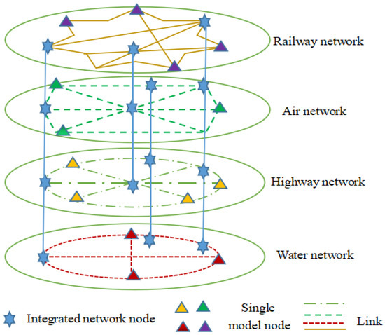
Figure 2.
Map of integrated transportation nodes and links.
In Figure 2, triangles of different colors indicate the nodes of a single transportation mode; the red triangles indicate the city nodes of the water transportation network, and the links of the same color denote the links among. Similarly, the yellow triangles, green triangles, and purple triangles indicate the city nodes of the highway network, air network, and railway network, respectively. Simultaneously, the links of the same color denote the links between cities that can be reached by highway, air, and railway modes, respectively. The blue hexagons denote the nodes of the integrated transportation network, and the links of the same color indicate multiple transportation modes passing through the same node city.
3.1. Establishment of the Railway Network
In this study, a railway transportation network connected by 277 railway lines was established between 44 node cities according to data from the China Railway website (https://ec.95306.cn/hycp/?active=0, accessed on 7 February 2023) and domestic cities serviced by CR Express. Figure 3 shows a topological map of the railway transportation network drawn using ArcGIS 10.2 software based on data from 277 railway transportation lines among the 44 node cities, which demonstrates the link network among cities serviced by CR Express or freight trains.
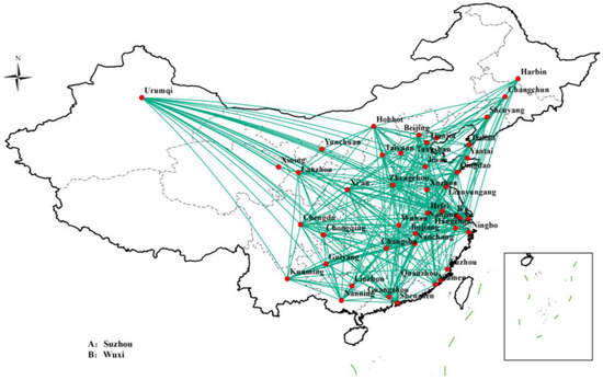
Figure 3.
Topological map of the railway transportation network.
3.2. Establishment of the Highway Network
To simplify the processing of the transportation network data and align with the reality of freight transportation, the expressway was primarily considered in this study. At present, the expressway network in China is laid out with radial lines and vertical and horizontal grids, which are composed of 7 radial lines starting from Beijing, as well as 9 north–south vertical lines and 18 east–west horizontal lines [34]. Compared with the railway transportation network, only cities directly connected by expressways are considered as the nodes of the highway network. Therefore, the cities connected by expressways are divided into segments. For example, the expressway between Beijing and Harbin passing through multiple node cities is divided into many subsections, such as Beijing–Tangshan, Tangshan–Shenyang, Shenyang–Changchun, and Changchun–Harbin. In addition, Dongguan is not connected by highway. Therefore, in this study, based on the above-mentioned factors, 79 connections among 43 node cities were identified. By using ArcGIS 10.2 software, a topological map of the expressway transportation network was drawn based on the 79 connections among the 43 node cities, as shown in Figure 4, which indicates the highway link network among the 43 node cities connected by the highway network.
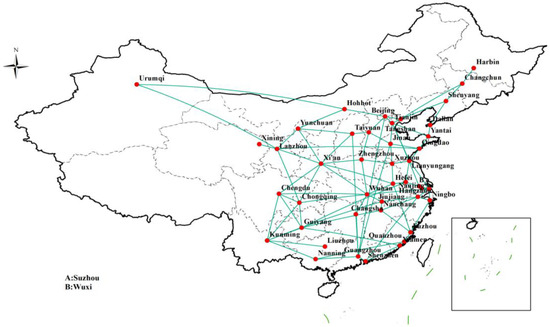
Figure 4.
Topological map of the expressway transportation network.
3.3. Establishment of the Air Network
Most airports in China are now dual-use airports for passengers and cargo; therefore, in this study, only the connections between the nodes of the aviation network were considered; the volume and frequency of freight transportation between the nodes were not considered. The data on the air transportation network primarily came from the direct routes between cities listed in the “Catalogue of Domestic Routes with Market-Adjusted Prices” published by the Chinese government. Many of these cities only have one airport, but some cities have multiple airports; cities with multiple airports were represented by the city name. For example, Pudong and Hongqiao airports in Shanghai were represented by Shanghai. Only one airline route was reserved between each pair of cities, and repetitive routes were deleted. After screening, since there are no airports in Dongguan, Tangshan, Jiujiang, and Suzhou, 462 direct routes were selected among 40 node cities in the air transportation network. A topological map of the air transportation network was drawn using ArcGIS 10.2 software based on the data from the 462 direct links among the 40 node cities, as shown in Figure 5, which denotes the air transportation network among the 40 node cities connected by the air network.
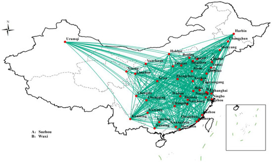
Figure 5.
Topological map of the air transportation network.
3.4. Establishment of the Waterway Network
Compared with railway, air, and highway transportation networks, water transportation is limited by geographical factors and not every node city has a mode of water transportation. Water transportation is generally divided into coastal and inland river transportation, but this study mainly considered the connection between ports. Domestic water transportation in China mainly involves inland river transport in the Heilongjiang, Yangtze, and Pearl River basins, as well as the Beijing–Hangzhou Grand Canal, and coastal shipping in coastal areas. However, because the Heilongjiang River basin is affected by geographical and climatic factors and the shipping scope is small, the port cities in the Heilongjiang River basin were not considered. The data used in this study were sourced from relevant government websites (for example, http://www.tcport.gov.cn/tcg/cjnh/zjgkwztt.sh-tml, accessed on 9 February 2023) and shipping companies (for example, http://www.chinaports.com/, accessed on 9 February 2023). Based on the above factors, 82 water transportation routes were identified among 27 port cities. Figure 6 is a topological map of the water transportation network drawn using ArcGIS 10.2 software based on the 82 water transportation links among the 27 port cities, which denotes the transportation network of direct water transportation links among the 27 port cities.
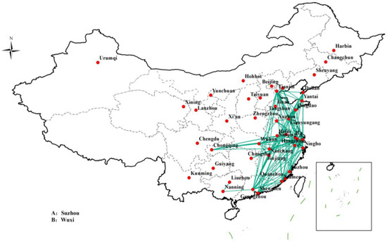
Figure 6.
Topological map of the water transportation network.
4. Evaluation Indicators
Given the complexity and diversity of evaluation factors, the impact of different evaluation indicators on the evaluation results is also different; therefore, the reasonable selection and use of evaluation indicators are crucial for obtaining scientific evaluation results. Considering the advantages and disadvantages of different evaluation indicators, based on references [25,27], this study selected six classic evaluation indicators from global and local perspectives, including closeness centrality, degree centrality, network constraint coefficient, betweenness centrality, clustering coefficient, and eigenvector centrality. The following are the six evaluation indicators:
- (1)
- Degree centrality
The centrality indicator degree centrality () measures the node’s influence, which is an essential parameter for studying the topology of complex networks. The number of the connection of individual node i is denoted as , that is, the number of links connected between node i and other nodes within the entire network. The maximum number of possible connections within the entire network is . The degree centrality indicates the ratio of to , as shown in Equation (2) [19,33].
where n is the number of nodes in the network. Generally, a node with a higher is directly connected to more nodes, thus occupying a more important position within the network.
- (2)
- Betweenness centrality ()
is the number of the shortest paths between the node and node d passing through an intermediate node i [13]. can be obtained from Equation (3):
where denotes the total number of shortest paths between node s and node d, and indicates the number of shortest paths between node s and d passing through node i. The higher the is, the more important vertex i is.
- (3)
- Closeness centrality ()
represents the reciprocal of the average distances of the shortest path between node i and all other nodes [33,35], which is defined as follows:
where is the minimum distance between node i and node j. The closer node i is to the network center, the greater becomes.
- (4)
- Eigenvector centrality ()
indicates the linear relationship between the centrality indicator of vertex i and the centrality metrics of the neighboring nodes [33], which is defined as follows:
where proportionality constant is the maximum eigenvalue of the nth-order adjacent matrix A = (. denotes the center vector of all vertices. The larger is, the more import node i is.
- (5)
- Clustering coefficient ()
reflects the tendency of node i to form clusters with its neighboring nodes, as shown in Equation (6). In general, only nodes with relatively low clustering coefficient values can become structural hole nodes [25].
where e(i) denotes the links number from node to its neighboring nodes. is the degree of node .
- (6)
- Network constraint coefficient ()
Burt put forward structural hole theory in 1992. The network constraint coefficient is an indicator used by Burt to reflect the number of structural holes and the extent of their impact on the information flow [36]. is defined as the influence of an individual node:
where q indicates the common adjacent node between node and ,. The proportional strength of node out of all the connections to node is denoted as . The sum of the proportions of indirect connections between node and is . The network constraint coefficient is defined as follows:
The higher is, the greater the probability that node i will become the central node.
5. The Integrated Evaluation Method
The TOPSIS is a multi-attribute decision-making approach employed by many scholars. However, it has some limitations. One limitation is that the accuracy of Euclidean distances is affected by the correlation between indicators. Another limitation is that it cannot accurately reflect the similarity of data curves. The GRA approach can not only capture non-linear relationships between sequences but also determine the level of closeness between system indicators. Therefore, the simplicity of the calculation of the TOPSIS approach and the similarity of the GRA approach were integrated into the multi-attribute decision approach. Moreover, the experience and knowledge of decision makers are seldom considered in the applications of the TOPSIS approach. Given these, this paper introduces Criteria Importance through the Intercriteria Correlation (CRITIC) objective weighting method into the combination of the TOPSIS and GRA. Then, this approach was combined with the indicators to assess the candidate consolidation centers of the integrated transportation network. The specific evaluation process is shown below.
- Step 1:
- Construction of indicator matrix
It is assumed that m indicators are employed to assess the importance of n nodes in the integrated transportation network. is the indicator value of each node. Here, and indicate the -th node and -th indicator separately, and the initial indicator matrix U = is shown in Equation (9):
- Step 2:
- Construction of normalized indicator matrix
Due to the presence of the evaluation indicators with different scales, the dimensionless indicator matrix is obtain by normalization.
where
- Step 3:
- Construction of indicator weight
To avoid the influence of individual preferences of evaluators on indicator weights, the CRITIC method proposed in [37] was employed in this study, and the concrete process is shown below.
- (1)
- Calculate the difference between evaluation indicators
The difference between evaluation indicators was calculated based on the normalized matrix constructed according to Equation (10). The CRITIC method uses the standard deviation to estimate the differential fluctuation between indicators i and j, as shown in Equation (12):
where denotes the average value of indicator j (column) and represents the standard deviation of indicator j. When the standard deviation between j and i is larger, it means that the information contained by indicator j is larger, which indicates that the evaluation intensity of indicator j is higher. Therefore, it is necessary to assign greater weight to indicator j. If the reverse is true, it is necessary to assign a smaller weight to indicator j.
- (2)
- Calculate the conflict between evaluation indicators
Similarly, the conflict between evaluation indicators was calculated based on the normalized matrix constructed according to Equation (10). The CRITIC method applies the correlation coefficient to estimate the conflict between indicator i and j. The stronger the correlation is, the smaller the conflict is, indicating that there is more identical information between indicators. Correspondingly, the evaluation intensity of indicator j is weakened to some extent, and therefore, less corresponding weight is assigned to indicator j. If the reverse is true, more weight is given. The equation for calculating the conflict between indicator j and other indicators is shown in Equations (13) and (14):
where denotes the correlation coefficient of indicator and . indicates the average value of indicator .
- (3)
- Calculate comprehensive information volume
The difference and conflict between indicators were calculated using Equations (12)–(14), and the information volume contained in the indicators was calculated using Equation (15) according to the difference and conflict.
Generally, the larger is, the more the information contained in indicator j, and the more important it is. In such cases, more weight should be assigned to the indicator. If the reverse is true, less weight should be assigned to the indicator.
- (4)
- Determine objective weight
The CRITIC was employed to determine the objective weight of the indicators in accordance with the comprehensive information on the differences and conflicts. Therefore, according to Equation (16), the indicator information volume contained in the j-th indicator is calculated to determine the corresponding weight , and the equation of calculation is shown below:
where is the weight of the indicator j.
- Step 4:
- Calculate the weighted normalization matrix
To effectively evaluate the influence of each indicator on the evaluation result, the normalized matrix constructed using Equation (10) and the weight of each indicator obtained from Equation (16) can be multiplied to obtain the weighted normalized matrix Z, as shown in Equation (17):
where represents the indicator value of the weighted normalized matrix, and indicates the dimensionless matrix.
- Step 5:
- Determine the ideal solutions
According to the weighted normalization matrix, the maximum and minimum of the various indicators are determined as the positive ideal solutions and the negative ideal solutions, , respectively.
- Step 6:
- Calculate the Euclidean distance
The weighted normalized matrix H was computed from Equation (17), and the positive ideal solution sets were obtained from Equation (18) and the negative ideal solution sets were obtained from Equation (19). Then, is labeled as the Euclidean distance of indicator j from the positive ideal solution, as shown in Equation (20). is labeled as the Euclidean distance of indicator j from the negative ideal solution, as shown in Equation (21).
- Step 7:
- Grey Relational Analysis (GRA)
- (1)
- Calculate grey relational coefficient
The grey relational coefficient is computed based on the weighted normalized matrix established by Equation (17). is expressed as the correlation coefficient between indicator j and the positive ideal sequence and is expressed as the correlation coefficient between indicator j and the negative ideal sequence. The calculation equations are shown in Equations (22) and (23).
where is the resolution coefficient that controls the degree of discrimination of the grey relational coefficient, and the value of ρ ranges from 0 to 1. The smaller ρ is, the greater the degree of discrimination is. The greater ρ is, the smaller the degree of discrimination is. The value of was set as 0.5 in this study.
- (2)
- Calculate grey relational degree
According to the grey relational coefficient, is the grey relational degree between indicator j and the positive ideal solution, while is the grey relational degree between indicator j and the negative ideal solution, which are expressed as Equations (24) and (25).
- Step 8:
- Dimensionless processing of , ,
, , are dimensionless values, and their specific calculations are shown in Equations (26)–(29).
- Step 9:
- Calculate the close degree
and were set as the proximity of the node i to the positive ideal solution and the negative ideal solution, respectively. Hence, the proximity of the node to the ideal solution was calculated in accordance with the dimensionless grey relational degree and dimensionless Euclidean distance. The calculation equations are shown in Equations (30) and (31):
where are the preference coefficients, which indicate the degree of preference of the decision maker. Generally, + = 1 and the values of are usually both 0.5.
Based on the above-mentioned comprehensive grey relational degree–Euclidean distance measure, the new measures obtained from Equations (30) and (31) were used to compute the relative closeness of each evaluation target. represents the target’s response to both the positive and negative ideal solutions in changing situations, and the calculation equation is shown in Equation (32). Finally, the targets were sorted based on the closeness value.
The greater is, the better the target’s evaluation is. Correspondingly, the smaller is, the poorer the target’s evaluation is.
6. Case Study
The purpose of the BRI is to enrich the transportation network and promote connection and cooperation around the world. Based on this background, a case study of the consolidation centers of an integrated transportation network composed of railway, road, water, and air routes was conducted to evaluate the above-mentioned approach.
6.1. Scoring and Ranking of the Candidate Consolidation Centers for a Single Mode
Firstly, according to the complex network theory, the raw data of the 44 node cities of the railway transportation network was normalized using Equation (10) in Section 5 in this paper, and then the CRITIC was employed to obtain the weights of six indicators of the railway transportation network according to Step 3 in Section 5. The concrete values of each indicator were 0.1939, 0.1363, 0.2029, 0.1994, 0.1335, and 0.1339. Similar to the process described above, the weights of the six indicators for the four transportation modes were calculated and are shown in Table 2.
Table 2.
Weights of indicators of railway, highway, air, and water networks.
Next, the weighted normalized matrix was obtained by multiplying the weights with the normalized matrix. Finally, the values of the six indicators for the 44 city nodes of the railway transportation network, including closeness centrality, eigenvector centrality, betweenness centrality, degree centrality, constraint coefficient, and clustering coefficient, were determined through the application of the combination of GRA and the TOPSIS. The concrete rankings are also shown in Table A6.
Similarly, the scores of the six indicators for the candidate consolidation centers of the highway, water, and air networks are also shown in Appendix B Table A7, Table A8 and Table A9. Table A6, Table A7, Table A8 and Table A9 show the indicator values, scores, and rankings of the six indicators for each candidate consolidation center in the railway transportation network, highway transportation network, air transportation network, and water transportation network, respectively.
6.2. Evaluation of the Single Transportation Mode Networks
To reflect the changes between the integrated transportation network and the single transportation mode networks, the candidate consolidation centers of the single transportation mode network were first evaluated and analyzed.
It can be seen from the overall rankings of the railway transportation network from Table A6 that more connections among the candidate consolidation centers resulted in higher rankings, which is in line with the clustering effect of complex network theory. These cities are important nodes in the Chinese domestic railway transportation network, which plays an important role in railway cargo transportation. In addition, China Railway Express (CR Express) mainly passes through ports such as Manzhouli, Erenhot, and Alashankou to reach Europe. However, from the perspective of geographical area, only Shenyang in Northeast China is in the top 50% and Manzhouli has not played its corresponding role as a port of CR Express due to distance reasons. Correspondingly, Urumqi and Xi’an are ranked high in Northwest China, indicating that the northwest land ports are regarded as the important outbound ports by the cities that are serviced by CR Express in China. Chengdu was one of the earliest cities in China to be serviced by CR Express, and it is also an important source of cargo consolidation centers. There are three cities in central China, Zhengzhou, Changsha, and Nanchang, which show the importance of the city’s geographical location. Currently, these cities have been the important Chinese starting points of CR Express. However, Beijing is not in the top 50%, because its main task is passenger transportation as the capital of China, despite its well-developed rail network.
The corresponding rankings of the candidate consolidation centers of the air transportation network are displayed in Table A7. The relevant indicator values for Suzhou, Dongguan, and Jiujiang were set to 0 due to them not having airports operating in air transportation. Similar to the railway transportation network, the more connections there are among node cities, the higher the rankings are. According to the geographical distribution of these cities, one can see that no cities were selected in the northwest region. The reasons are the vast territory, sparse population, backward economic development, or low industrial concentration. In addition, there are a few exceptions. Shanghai and Xi’an are not in the top 50%, although there are more routes among node cities. The reason is that these cities are affected by the direct routes, and the values of structural holes of these direct routes and other indicators are relatively low, resulting in their low ranking.
Table A8 shows the corresponding rankings of the candidate consolidation centers of the highway transportation network. Based on the geographical distribution of these cities, the cities in Northeast China are all in the bottom 50%. The reason is that there are fewer national highway connections between cities in the northeast and cities in other regions. Additionally, the relevant indicator values for Dongguan were set to 0 because Dongguan is not connected by the national highway. However, Beijing is at the forefront of the ranking in the highway network because, as the capital of China, the highway network is centered around Beijing.
Due to the particularity of water transportation, the relevant indicator values for cities with no water transportation modes passing through were set to 0. Meanwhile, Harbin is an inland river transportation city with a relatively small freight volume, mainly connecting some ports in Russia and not directly connected with other Chinese domestic node cities. Therefore, the relevant indicator value for Harbin was also set to 0. Therefore, there were 27 node cities in the water transportation network. As shown in Table A9, the rankings of the 27 candidate consolidation centers were determined based on the indicator values. It can be seen from the ranking that there were no node cities in Northwest China and Northeast China due to the lack of water transportation. Correspondingly, most of the selected node cities are mainly located in the coastal areas and some selected cities are located in the Yangtze River basin. The node cities in coastal areas were relatively high in the overall ranking of the water transportation network.
6.3. Comprehensive Evaluation of the Integrated Transportation Network
This study evaluated and ranked the candidate consolidation centers in an integrated transportation network under the BRI. This ranking can supply a reference for optimizing the layout of these centers to some extent, thereby enhancing the efficiency of freight services in China. We assessed the overall conditions of various transportation modes in each node city following the evaluation obtained for each mode individually. A comprehensive evaluation was conducted on the transportation modes passing through the candidate consolidation centers to obtain the ranking of these cities under the BRI.
Given that freight volume is an important indicator of transportation business and industry linkage, this study referred to references [11] and [27] and the proportion of freight volume of different transportation modes to the total freight volume in 2022 published by the Chinese government as the weight of each transportation mode [38]. After calculation, the proportions of railway, highway, water, and air freight volumes to total freight volume were 0.097419, 0.733509, 0.168952, and 0.000120, respectively. The comprehensive score of each node city can be obtained based on these weights. Consequently, the comprehensive score () of each node city of the integrated transportation network was calculated using Equation (33).
where , , and represent the comprehensive score for each city in the highway, railway, water, and air transportation networks, respectively.
In summary, 44 candidate consolidation centers were comprehensively evaluated based on each transportation mode within the integrated transportation network under the BRI with the freight volumes serving as the weights. The final comprehensive scores and rankings of the 44 node cities are displayed in Table 3.
Table 3.
Comprehensive score and ranking of each node city.
Based on the spatial layout and government policies under the BRI, with reference to [11], five attributes were employed to analyze the selection of candidate consolidation centers, including service by CR Express, along inland river, along the coast, along the key railway, and the final comprehensive score. Finally, the ten major cities, including Wuhan, Chongqing, Tianjin, Shanghai, Guangzhou, Yantai, Hangzhou, Lianyungang, Hefei, and Dalian, were selected as consolidation centers of the integrated transportation network in this study. On the other hand, the straight-line distance from Yantai to Dalian is only 170 km, and Hangzhou is about 170 km away from Shanghai. Considering the related geographical factors, Shanghai was merged with Hangzhou and Yantai was merged with Dalian. Wuhan, Chongqing, Tianjin, Shanghai, Guangzhou, Lianyungang, Hefei, and Dalian were finally recommended as the consolidation centers of the integrated transportation network, and Figure 7 shows the final selection results. Additionally, one can see that the top node cities are located along the inland river or coastal areas from Table 3. Xi’an, ranked 19th, is the top-ranked inland city without water transport, which indicates that the absence of water transport weakens the competitiveness of inland cities in the integrated transportation network. In addition, by comparing the top-ranked cities in the integrated transportation network with those in the single-mode networks, it can be observed that many of the top cities in the integrated network ranking are also among the top cities in the single-mode network rankings, indicating that the cities that hold important positions in the single-mode networks continue to maintain their significant status in the integrated network as well, such as Wuhan, Chongqing, Tianjin, Shanghai, and Guangzhou. At the same time, the ranking results revealed that the competitiveness of a node city increases as it accommodates more transportation modes. Consequently, the city’s cargo turnover capacity within the entire transportation network also strengthens.
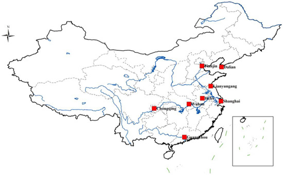
Figure 7.
Topological map of location of consolidation centers.
7. Discussion
It is well known that the feasibility of results can be confirmed by the applied evaluation method. In this subsection, an evaluation was performed with the TOPSIS to validate the rationality and accuracy of the proposed GRA–TOPSIS method. Table 4 indicates the comparison results of the two different methods.
Table 4.
Ranking results for different methods.
It can be seen that Wuhan, Chongqing, Guangzhou, Tianjin, Shanghai, and Yantai were always the best candidate cities for consolidation centers in the integrated transportation network. In contrast, Zhengzhou, Urumqi, Shijiazhuang, Yinchuan, Changchun, Taiyuan, and Hohhot were all the least suitable locations for consolidation centers as indicated by the comparison of the two methods. Moreover, some cities such as Xi’an, Harbin, Lanzhou, Kunming, Xiamen, Dongguan, Xining, Shenzhen, Chengdu, and others showed significant changes when their results were compared. The reasons for the above situation are the limited transportation modes or routes, and the results could be reflected by the core ideas of these two methods. Specifically, the GRA–TOPSIS approach focuses on the distance between alternative solutions and the connection between standards. The TOPSIS mainly considers the distance between alternative reference schemes and the best reference scheme.
Additionally, to compare the result obtained using the two methods, Kendall’s tau correlation coefficient (KTC) was applied to study the difference in accuracy between the two methods [39]. The value of the calculated KTC of the two methods was 0.661734. It can be concluded that the obtained rankings have a high correlation with each other. Meanwhile, the reliability of an evaluation method was also demonstrated based on the distinction degree of the evaluation methods [40]. Accordingly, the values of the GRA–TOPSIS and TOPSIS methods were 1.075746 and 1.075126, respectively. The value of the GRA–TOPSIS was greater than that of the TOPSIS and then the reliability of the GRA–TOPSIS is relatively better than that of the TOPSIS. Table 5 and Table 6 show the values of KTC and distinction degree, respectively.
Table 5.
KTC of GRA-TOPSIS and TOPSIS.
Table 6.
Distinction degree of GRA-TOPSIS and TOPSIS.
8. Conclusions
The selection of the consolidation centers in the integrated transportation network under the BRI was evaluated in this paper, with the aim to reduce freight transportation costs and improve the efficiency of logistics operations. First of all, 44 node cities were selected based on the relevant national policies. Then, the transportation networks composed of railway, air, highway, and water routes were constructed. Based on the above work, the corresponding indicators were determined according to complex network theory, and the weights of these indicators were also determined based on the CRITIC approach. Then, the TOPSIS and GRA methods were combined to calculate data on the different transportation modes of each node city. Next, the proportion of the freight volume of the different transportation modes to the total freight volume in 2022 published by the Chinese government was used as the weight of each transportation mode to calculate the comprehensive score of each node city. The results showed that there are the top-ranked node cities in the integrated transportation network are all intersections of the four transportation modes, and most of them are located in inland rivers or coastal areas, indicating that inland river and coastal shipping play an important role in cargo transportation. Additionally, it also indicates that the absence of water transportation weakens the competitiveness of inland cities. Finally, based on the comprehensive consideration, Wuhan, Chongqing, Tianjin, Shanghai, Guangzhou, Lianyungang, Hefei, and Dalian were recommended as the consolidation centers of the integrated transportation network. Moreover, the GRA-TOPSIS method was found to be better than the TOPSIS through Kendall’s tau correlation coefficient and the distinction degree based on the comparison between the GRA-TOPSIS and TOPSIS methods. Additionally, this study can also provide some reference for other countries with transportation networks similar to those of China.
This paper has covered transportation modes such as rail, water, air, and highway when evaluating the consolidation center of the integrated transportation network. However, there are still some limitations that require further study. For example, more factors could be considered when choosing the candidate consolidation centers, such as industrial output value, economic scale, export scale, and the distance between cities. On the other hand, more indicators could be considered for urban population, transportation cost, the impact on urban environments, the carrying capacity of the transportation mode, and the traffic conditions of the node cities in future research. It is hoped that this result can provide some insights for the government to outline and build consolidation centers for an integrated transportation network composed of railway, air, highway, and water routes and for enterprises to choose transportation routes.
Author Contributions
Conceptualization, Q.Y. and Y.X.; Data curation, Q.Y. and Y.X.; Formal analysis, Q.Y.; Funding acquisition, G.W.; Investigation, Q.Y.; Methodology, Q.Y.; Project administration, Q.Y. and G.W.; Resources, Q.Y.; Software, Q.Y.; Supervision, G.W.; Validation, Q.Y.; Visualization, Y.X.; Writing—original draft, Q.Y.; Writing—review and editing, Q.Y. and G.W. All authors have read and agreed to the published version of the manuscript.
Funding
This research was funded by the National Natural Science Foundation of China (72071184).
Institutional Review Board Statement
Not applicable.
Informed Consent Statement
Not applicable.
Data Availability Statement
The data in this paper are partly from the references (see the corresponding descriptions) and from the following websites: https://ec.95306.cn/hycp/?active=0 (accessed on 7 February 2023); http://www.chinaports.com/ (accessed on 9 February 2023); http://www.tcport.gov.cn/tcg/cjnh/zjgkwztt.sh-tml (accessed on 9 February 2023); http://www.cecs.org.cn/zhxw/7729.html (accessed on 11 February 2023); https://xxgk.mot.gov.cn/2020/jigou/zhghs/202308/t20230825_3899151.html (accessed on 13 February 2023); https://www.mnr.gov.cn/zt/hd/chfxcr/gcdtgltl_29657/gjbtzs/201608/t20160811_2130097.html (accessed on 14 February 2023).
Acknowledgments
We express our sincere gratitude to the reviewers and editors for their constructive comments and valuable suggestions, which have greatly improved the quality of our manuscript.
Conflicts of Interest
The authors declare no conflicts of interest.
Appendix A
Table A1.
List of national or regional logistics node cities.
Table A1.
List of national or regional logistics node cities.
| No. | City | Node City | No. | City | Node City |
|---|---|---|---|---|---|
| 1 | Chongqing | National logistics node city | 23 | Xining | National logistics node city |
| 2 | Wuhan | National logistics node city | 24 | Tianjin | National logistics node city |
| 3 | Zhengzhou | National logistics node city | 25 | Taiyuan | National logistics node city |
| 4 | Suzhou | National logistics node city | 26 | Shenzhen | National logistics node city |
| 5 | Guangzhou | National logistics node city | 27 | Jinan | National logistics node city |
| 6 | Xi’an | National logistics node city | 28 | Shanghai | National logistics node city |
| 7 | Hefei | National logistics node city | 29 | Tangshan | Regional logistics node city |
| 8 | Shenyang | National logistics node city | 30 | Shijiazhuang | National logistics node city |
| 9 | Ningbo | National logistics node city | 31 | Chengdu | National logistics node city |
| 10 | Changsha | National logistics node city | 32 | Yinchuan | National logistics node city |
| 11 | Lianyungang | Regional logistics node city | 33 | Nanning | National logistics node city |
| 12 | Urumqi | National logistics node city | 34 | Hohhot | National logistics node city |
| 13 | Harbin | National logistics node city | 35 | Hangzhou | National logistics node city |
| 14 | Lanzhou | National logistics node city | 36 | Fuzhou | National logistics node city |
| 15 | Qingdao | National logistics node city | 37 | Guiyang | National logistics node city |
| 16 | Kunming | National logistics node city | 38 | Beijing | National logistics node city |
| 17 | Xiamen | National logistics node city | 39 | Xuzhou | Regional logistics node city |
| 18 | Changchun | National logistics node city | 40 | Quanzhou | Regional logistics node city |
| 19 | Nanchang | National logistics node city | 41 | Jiujiang | Regional logistics node city |
| 20 | Dalian | National logistics node city | 42 | Yantai | Regional logistics node city |
| 21 | Dongguan | Regional logistics node city | 43 | Liuzhou | Regional logistics node city |
| 22 | Nanjing | National logistics node city | 44 | Wuxi | Regional logistics node city |
Source: China Association for Engineering Construction Standardization (http://www.cecs.org.cn/zhxw/7729.html, accessed on 11 February 2023).
Table A2.
List of node cities of CR Express.
Table A2.
List of node cities of CR Express.
| No. | City | Node City | No. | City | Node City |
|---|---|---|---|---|---|
| 1 | Chongqing | Node city of CR Express | 23 | Xining | Node city of CR Express |
| 2 | Wuhan | Node city of CR Express | 24 | Tianjin | Node city of CR Express |
| 3 | Zhengzhou | Node city of CR Express | 25 | Taiyuan | Node city of CR Express |
| 4 | Suzhou | Node city of CR Express | 26 | Shenzhen | Node city of CR Express |
| 5 | Guangzhou | Node city of CR Express | 27 | Jinan | Node city of CR Express |
| 6 | Xi’an | Node city of CR Express | 28 | Shanghai | Node city of CR Express |
| 7 | Hefei | Node city of CR Express | 29 | Tangshan | Node city of CR Express |
| 8 | Shenyang | Node city of CR Express | 30 | Shijiazhuang | Node city of CR Express |
| 9 | Ningbo | Node city of CR Express | 31 | Chengdu | Node city of CR Express |
| 10 | Changsha | Node city of CR Express | 32 | Yinchuan | Node city of CR Express |
| 11 | Lianyungang | Node city of CR Express | 33 | Nanning | Node city of CR Express |
| 12 | Urumqi | Node city of CR Express | 34 | Hohhot | Node city of CR Express |
| 13 | Harbin | Node city of CR Express | 35 | Hangzhou | Node city of CR Express |
| 14 | Suzhou | Node city of CR Express | 36 | Fuzhou | Node city of CR Express |
| 15 | Qingdao | Node city of CR Express | 37 | Guiyang | Node city of CR Express |
| 16 | Kunming | Node city of CR Express | 38 | Beijing | Node city of CR Express |
| 17 | Xiamen | Node city of CR Express | 39 | Xuzhou | Node city of CR Express |
| 18 | Changchun | Node city of CR Express | 40 | Quanzhou | Node city of CR Express |
| 19 | Nanchang | Node city of CR Express | 41 | Jiujiang | Node city of CR Express |
| 20 | Dalian | Node city of CR Express | 42 | Yantai | Node city of CR Express |
| 21 | Dongguan | Node city of CR Express | 43 | Liuzhou | Node city of CR Express |
| 22 | Nanjing | Node city of CR Express | 44 | Wuxi | Node city of CR Express |
Source: 95306 China Railway (https://ec.95306.cn/hycp/?active=0, accessed on 7 February 2023).
Table A3.
List of node cities of water transportation.
Table A3.
List of node cities of water transportation.
| No. | City | Node Type | No. | City | Node Type |
|---|---|---|---|---|---|
| 1 | Chongqing | Inland river node city | 15 | Tianjin | Coastal node city |
| 2 | Wuhan | Inland river node city | 16 | Shenzhen | Coastal node city |
| 3 | Suzhou | Inland river node city | 17 | Shanghai | Coastal node city |
| 4 | Guangzhou | Coastal node city | 18 | Tangshan | Inland river node city |
| 5 | Hefei | Inland river node city | 19 | Nanning | Inland river node city |
| 6 | Ningbo | Coastal node city | 20 | Hangzhou | Coastal node city |
| 7 | Changsha | Inland river node city | 21 | Fuzhou | Coastal node city |
| 8 | Lianyungang | Coastal node city | 22 | Xuzhou | Inland river node city |
| 9 | Qingdao | Coastal node city | 23 | Quanzhou | Coastal node city |
| 10 | Xiamen | Coastal node city | 24 | Jiujiang | Inland river node city |
| 11 | Nanchang | Inland river node city | 25 | Yantai | Coastal node city |
| 12 | Dalian | Coastal node city | 26 | Liuzhou | Inland river node city |
| 13 | Dongguan | Inland river node city | 27 | Wuxi | Inland river node city |
| 14 | Nanjing | Inland river node city | 28 |
Source: Ministry of Transport of the People’s Republic of China (https://xxgk.mot.gov.cn/2020/jigou/zhghs/202308/t20230825_3899151.html, accessed on 13 February 2023).
Table A4.
List of node cities of air transportation.
Table A4.
List of node cities of air transportation.
| No. | City | Node Type | No. | City | Node Type |
|---|---|---|---|---|---|
| 1 | Chongqing | Air node city | 21 | Xining | Air node city |
| 2 | Wuhan | Air node city | 22 | Tianjin | Air node city |
| 3 | Zhengzhou | Air node city | 23 | Taiyuan | Air node city |
| 4 | Guangzhou | Air node city | 24 | Shenzhen | Air node city |
| 5 | Xi’an | Air node city | 25 | Jinan | Air node city |
| 6 | Hefei | Air node city | 26 | Shanghai | Air node city |
| 7 | Shenyang | Air node city | 27 | Shijiazhuang | Air node city |
| 8 | Ningbo | Air node city | 28 | Chengdu | Air node city |
| 9 | Changsha | Air node city | 29 | Yinchuan | Air node city |
| 10 | Lianyungang | Air node city | 30 | Nanning | Air node city |
| 11 | Urumqi | Air node city | 31 | Hohhot | Air node city |
| 12 | Harbin | Air node city | 32 | Hangzhou | Air node city |
| 13 | Lanzhou | Air node city | 33 | Fuzhou | Air node city |
| 14 | Qingdao | Air node city | 34 | Guiyang | Air node city |
| 15 | Kunming | Air node city | 35 | Beijing | Air node city |
| 16 | Xiamen | Air node city | 36 | Xuzhou | Air node city |
| 17 | Changchun | Air node city | 37 | Jiujiang | Air node city |
| 18 | Nanchang | Air node city | 38 | Yantai | Air node city |
| 19 | Dalian | Air node city | 39 | Liuzhou | Air node city |
| 20 | Nanjing | Air node city | 40 | Wuxi | Air node city |
Source: Civil Aviation Administration of China [41].
Table A5.
List of provincial capitals.
Table A5.
List of provincial capitals.
| No. | City | Node Type | No. | City | Node Type |
|---|---|---|---|---|---|
| 1 | Chongqing | Municipality | 16 | Xining | Provincial capital |
| 2 | Wuhan | Provincial capital | 17 | Tianjin | Municipality |
| 3 | Zhengzhou | Provincial capital | 18 | Taiyuan | Provincial capital |
| 4 | Guangzhou | Provincial capital | 19 | Jinan | Provincial capital |
| 5 | Xi’an | Provincial capital | 20 | Shanghai | Municipality |
| 6 | Hefei | Provincial capital | 21 | Shijiazhuang | Provincial capital |
| 7 | Shenyang | Provincial capital | 22 | Chengdu | Provincial capital |
| 8 | Changsha | Provincial capital | 23 | Yinchuan | Provincial capital |
| 9 | Urumqi | Provincial capital | 24 | Nanning | Provincial capital |
| 10 | Harbin | Provincial capital | 25 | Hohhot | Provincial capital |
| 11 | Lanzhou | Provincial capital | 26 | Hangzhou | Provincial capital |
| 12 | Kunming | Provincial capital | 27 | Fuzhou | Provincial capital |
| 13 | Changchun | Provincial capital | 28 | Guiyang | Provincial capital |
| 14 | Nanchang | Provincial capital | 29 | Beijing | Municipality |
| 15 | Nanjing | Provincial capital | 30 |
Source: Ministry of National Resources of the People’s Republic of China (https://www.mnr.gov.cn/zt/hd/chfxcr/gcdtgltl_29657/gjbtzs/201608/t20160811_2130097.html, accessed on 14 February 2023).
Appendix B
Table A6.
Values of indicators of railway transportation network.
Table A6.
Values of indicators of railway transportation network.
| No. | City | Degree | Degree Centrality | Betweenness Centrality | Closeness Centrality | Eigenvector Centrality | Constraint Coefficient | Clustering Coefficient | Comprehensive Score of Railway Network | Ranking |
|---|---|---|---|---|---|---|---|---|---|---|
| 1 | Chongqing | 13 | 0.302326 | 0.007049 | 0.573333 | 0.138340 | 0.147733 | 0.589744 | 0.468878 | 26 |
| 2 | Wuhan | 17 | 0.395349 | 0.023898 | 0.623188 | 0.171448 | 0.128758 | 0.514706 | 0.483948 | 13 |
| 3 | Zhengzhou | 26 | 0.604651 | 0.045035 | 0.716667 | 0.247857 | 0.111981 | 0.455385 | 0.495845 | 8 |
| 4 | Suzhou | 16 | 0.372093 | 0.013435 | 0.614286 | 0.166533 | 0.131415 | 0.541667 | 0.481240 | 17 |
| 5 | Guangzhou | 24 | 0.558140 | 0.055312 | 0.693548 | 0.226815 | 0.112617 | 0.445652 | 0.500474 | 6 |
| 6 | Xi’an | 23 | 0.534884 | 0.018487 | 0.682540 | 0.241499 | 0.124304 | 0.561265 | 0.506751 | 3 |
| 7 | Hefei | 14 | 0.325581 | 0.006573 | 0.573333 | 0.152294 | 0.145876 | 0.615385 | 0.477620 | 20 |
| 8 | Shenyang | 15 | 0.348837 | 0.014351 | 0.581081 | 0.135663 | 0.151742 | 0.514286 | 0.480288 | 18 |
| 9 | Ningbo | 15 | 0.348837 | 0.013626 | 0.597222 | 0.156819 | 0.141121 | 0.590476 | 0.483715 | 14 |
| 10 | Changsha | 22 | 0.511628 | 0.028515 | 0.671875 | 0.220099 | 0.126504 | 0.523810 | 0.504486 | 4 |
| 11 | Lianyungang | 9 | 0.209302 | 0.003035 | 0.551282 | 0.099512 | 0.175169 | 0.638889 | 0.454819 | 38 |
| 12 | Urumqi | 26 | 0.604651 | 0.097795 | 0.716667 | 0.237736 | 0.108931 | 0.421538 | 0.507032 | 2 |
| 13 | Harbin | 9 | 0.209302 | 0.009000 | 0.537500 | 0.074581 | 0.171475 | 0.444444 | 0.454941 | 37 |
| 14 | Lanzhou | 16 | 0.372093 | 0.029593 | 0.614286 | 0.150493 | 0.135311 | 0.458333 | 0.475377 | 22 |
| 15 | Qingdao | 23 | 0.534884 | 0.031140 | 0.682540 | 0.224187 | 0.119908 | 0.486166 | 0.499621 | 7 |
| 16 | Kunming | 15 | 0.348837 | 0.011352 | 0.597222 | 0.149395 | 0.145318 | 0.571429 | 0.478006 | 19 |
| 17 | Xiamen | 15 | 0.348837 | 0.016713 | 0.605634 | 0.146181 | 0.125621 | 0.447619 | 0.466563 | 29 |
| 18 | Changchun | 10 | 0.232558 | 0.004698 | 0.544304 | 0.085074 | 0.199911 | 0.622222 | 0.457503 | 35 |
| 19 | Nanchang | 23 | 0.534884 | 0.031356 | 0.682540 | 0.227865 | 0.123532 | 0.513834 | 0.503000 | 5 |
| 20 | Dalian | 8 | 0.186047 | 0.003583 | 0.511905 | 0.065188 | 0.220170 | 0.607143 | 0.458258 | 33 |
| 21 | Dongguan | 3 | 0.069767 | 0.000000 | 0.472527 | 0.036872 | 0.397977 | 1.000000 | 0.450085 | 40 |
| 22 | Nanjing | 20 | 0.465116 | 0.040724 | 0.651515 | 0.184936 | 0.118198 | 0.436842 | 0.492756 | 11 |
| 23 | Xining | 2 | 0.046512 | 0.000000 | 0.430000 | 0.022584 | 0.551827 | 1.000000 | 0.457530 | 34 |
| 24 | Tianjin | 25 | 0.581395 | 0.065271 | 0.704918 | 0.215978 | 0.113469 | 0.403333 | 0.495618 | 9 |
| 25 | Taiyuan | 14 | 0.325581 | 0.004659 | 0.573333 | 0.150739 | 0.150503 | 0.637363 | 0.476714 | 21 |
| 26 | Shenzhen | 17 | 0.395349 | 0.021504 | 0.623188 | 0.169303 | 0.133101 | 0.514706 | 0.484054 | 12 |
| 27 | Jinan | 19 | 0.441860 | 0.032107 | 0.641791 | 0.168003 | 0.122759 | 0.438596 | 0.483260 | 15 |
| 28 | Shanghai | 20 | 0.465116 | 0.032380 | 0.651515 | 0.194503 | 0.115797 | 0.457895 | 0.493701 | 10 |
| 29 | Tangshan | 6 | 0.139535 | 0.000929 | 0.472527 | 0.045667 | 0.269930 | 0.733333 | 0.455568 | 36 |
| 30 | Shijiazhuang | 10 | 0.232558 | 0.001965 | 0.551282 | 0.105552 | 0.175782 | 0.666667 | 0.458857 | 31 |
| 31 | Chengdu | 22 | 0.511628 | 0.016248 | 0.671875 | 0.232521 | 0.129773 | 0.588745 | 0.509849 | 1 |
| 32 | Yinchuan | 3 | 0.069767 | 0.000143 | 0.462366 | 0.030719 | 0.384650 | 0.666667 | 0.432786 | 42 |
| 33 | Nanning | 15 | 0.348837 | 0.006503 | 0.605634 | 0.163758 | 0.154230 | 0.666667 | 0.481669 | 16 |
| 34 | Hohhot | 17 | 0.395349 | 0.044308 | 0.614286 | 0.139838 | 0.114371 | 0.345588 | 0.470704 | 25 |
| 35 | Hangzhou | 12 | 0.279070 | 0.011596 | 0.544304 | 0.103557 | 0.155106 | 0.439394 | 0.466891 | 28 |
| 36 | Fuzhou | 7 | 0.162791 | 0.005679 | 0.511905 | 0.054375 | 0.174249 | 0.238095 | 0.428890 | 43 |
| 37 | Guiyang | 10 | 0.232558 | 0.001753 | 0.524390 | 0.105467 | 0.196212 | 0.755556 | 0.472797 | 23 |
| 38 | Beijing | 15 | 0.348837 | 0.014928 | 0.597222 | 0.143288 | 0.133323 | 0.485714 | 0.471305 | 24 |
| 39 | Xuzhou | 8 | 0.186047 | 0.003215 | 0.524390 | 0.072299 | 0.194695 | 0.535714 | 0.452254 | 39 |
| 40 | Quanzhou | 5 | 0.116279 | 0.002304 | 0.518072 | 0.046195 | 0.260505 | 0.600000 | 0.427987 | 44 |
| 41 | Jiujiang | 5 | 0.116279 | 0.000123 | 0.483146 | 0.052814 | 0.289660 | 0.900000 | 0.458679 | 32 |
| 42 | Yantai | 6 | 0.139535 | 0.000154 | 0.500000 | 0.070883 | 0.242848 | 0.866667 | 0.467560 | 27 |
| 43 | Liuzhou | 8 | 0.186047 | 0.001409 | 0.524390 | 0.090434 | 0.203046 | 0.714286 | 0.461740 | 30 |
| 44 | Wuxi | 6 | 0.139535 | 0.001638 | 0.505882 | 0.049560 | 0.242902 | 0.600000 | 0.440172 | 41 |
Table A7.
Value of indicators of air transportation network.
Table A7.
Value of indicators of air transportation network.
| No. | City | Degree | Degree Centrality | Betweenness Centrality | Closeness Centrality | Eigenvector Centrality | Constraint Coefficient | Clustering Coefficient | Comprehensive Score of Air Network | Ranking |
|---|---|---|---|---|---|---|---|---|---|---|
| 1 | Chongqing | 34 | 0.790698 | 0.022157 | 0.808898 | 0.207518 | 0.107610 | 0.691622 | 0.504407 | 12 |
| 2 | Wuhan | 27 | 0.627907 | 0.013749 | 0.702062 | 0.167107 | 0.111167 | 0.706553 | 0.507661 | 8 |
| 3 | Zhengzhou | 29 | 0.674419 | 0.011407 | 0.729594 | 0.178043 | 0.106081 | 0.677340 | 0.501550 | 14 |
| 4 | Suzhou | 0 | 0.000000 | 0.000000 | 0.000000 | 0.000000 | 0.000000 | 0.000000 | 0.000000 | 42 |
| 5 | Guangzhou | 26 | 0.604651 | 0.005700 | 0.689061 | 0.166030 | 0.113788 | 0.756923 | 0.498788 | 19 |
| 6 | Xi’an | 33 | 0.767442 | 0.014321 | 0.791687 | 0.201866 | 0.106578 | 0.687500 | 0.494832 | 23 |
| 7 | Hefei | 22 | 0.511628 | 0.003839 | 0.641540 | 0.143496 | 0.114765 | 0.761905 | 0.484910 | 32 |
| 8 | Shenyang | 26 | 0.604651 | 0.012175 | 0.689061 | 0.163483 | 0.107634 | 0.707692 | 0.500712 | 15 |
| 9 | Ningbo | 18 | 0.418605 | 0.003174 | 0.600150 | 0.118785 | 0.122546 | 0.797386 | 0.482786 | 34 |
| 10 | Changsha | 32 | 0.744186 | 0.025009 | 0.775194 | 0.191227 | 0.102516 | 0.645161 | 0.513417 | 4 |
| 11 | Lianyungang | 9 | 0.209302 | 0.001655 | 0.516796 | 0.053307 | 0.159907 | 0.555556 | 0.457044 | 38 |
| 12 | Urumqi | 22 | 0.511628 | 0.004388 | 0.641540 | 0.141381 | 0.117314 | 0.761905 | 0.489342 | 28 |
| 13 | Harbin | 28 | 0.651163 | 0.005532 | 0.715564 | 0.181860 | 0.112862 | 0.777778 | 0.504578 | 11 |
| 14 | Lanzhou | 26 | 0.604651 | 0.004896 | 0.689061 | 0.169007 | 0.111967 | 0.766154 | 0.497409 | 21 |
| 15 | Qingdao | 30 | 0.697674 | 0.023128 | 0.744186 | 0.184530 | 0.106520 | 0.694253 | 0.525641 | 1 |
| 16 | Kunming | 34 | 0.790698 | 0.024978 | 0.808898 | 0.207101 | 0.106987 | 0.689840 | 0.508767 | 7 |
| 17 | Xiamen | 24 | 0.558140 | 0.003118 | 0.664452 | 0.160177 | 0.116026 | 0.811594 | 0.490206 | 26 |
| 18 | Changchun | 20 | 0.465116 | 0.006532 | 0.620155 | 0.129466 | 0.115638 | 0.747368 | 0.489678 | 27 |
| 19 | Nanchang | 28 | 0.651163 | 0.016774 | 0.715564 | 0.171219 | 0.107440 | 0.687831 | 0.511331 | 6 |
| 20 | Dalian | 31 | 0.720930 | 0.024997 | 0.759374 | 0.186932 | 0.104769 | 0.666667 | 0.520965 | 2 |
| 21 | Dongguan | 0 | 0.000000 | 0.000000 | 0.000000 | 0.000000 | 0.000000 | 0.000000 | 0.000000 | 42 |
| 22 | Nanjing | 30 | 0.697674 | 0.014936 | 0.744186 | 0.182812 | 0.104540 | 0.668966 | 0.505921 | 9 |
| 23 | Xining | 10 | 0.232558 | 0.000190 | 0.524075 | 0.068746 | 0.165443 | 0.911111 | 0.482772 | 35 |
| 24 | Tianjin | 27 | 0.627907 | 0.008963 | 0.702062 | 0.170361 | 0.109642 | 0.726496 | 0.499631 | 16 |
| 25 | Taiyuan | 26 | 0.604651 | 0.004522 | 0.689061 | 0.169759 | 0.113734 | 0.781538 | 0.497693 | 20 |
| 26 | Shenzhen | 32 | 0.744186 | 0.020495 | 0.775194 | 0.195552 | 0.108230 | 0.693548 | 0.512061 | 5 |
| 27 | Jinan | 21 | 0.488372 | 0.002576 | 0.630666 | 0.140005 | 0.118750 | 0.809524 | 0.482850 | 33 |
| 28 | Shanghai | 33 | 0.767442 | 0.014887 | 0.791687 | 0.202652 | 0.107103 | 0.696970 | 0.496730 | 22 |
| 29 | Tangshan | 5 | 0.116279 | 0.000215 | 0.471004 | 0.030302 | 0.240696 | 0.600000 | 0.453250 | 41 |
| 30 | Shijiazhuang | 21 | 0.488372 | 0.007760 | 0.630666 | 0.128840 | 0.113221 | 0.685714 | 0.485398 | 30 |
| 31 | Chengdu | 32 | 0.744186 | 0.011791 | 0.775194 | 0.199600 | 0.109484 | 0.721774 | 0.499575 | 17 |
| 32 | Yinchuan | 20 | 0.465116 | 0.002538 | 0.620155 | 0.132878 | 0.123724 | 0.826316 | 0.485644 | 29 |
| 33 | Nanning | 25 | 0.581395 | 0.003217 | 0.676533 | 0.166405 | 0.117022 | 0.820000 | 0.494052 | 24 |
| 34 | Hohhot | 21 | 0.488372 | 0.001475 | 0.630666 | 0.144287 | 0.122168 | 0.871429 | 0.485132 | 31 |
| 35 | Hangzhou | 30 | 0.697674 | 0.014640 | 0.744186 | 0.182050 | 0.105157 | 0.668966 | 0.505550 | 10 |
| 36 | Fuzhou | 19 | 0.441860 | 0.004997 | 0.600150 | 0.123659 | 0.124252 | 0.795322 | 0.499014 | 18 |
| 37 | Guiyang | 27 | 0.627907 | 0.004663 | 0.702062 | 0.176297 | 0.116645 | 0.800570 | 0.504032 | 13 |
| 38 | Beijing | 32 | 0.744186 | 0.029049 | 0.775194 | 0.188191 | 0.103704 | 0.637097 | 0.520587 | 3 |
| 39 | Xuzhou | 7 | 0.162791 | 0.000610 | 0.509716 | 0.042801 | 0.199387 | 0.714286 | 0.456481 | 39 |
| 40 | Quanzhou | 13 | 0.302326 | 0.000670 | 0.547196 | 0.089531 | 0.137968 | 0.820513 | 0.476879 | 36 |
| 41 | Jiujiang | 0 | 0.000000 | 0.000000 | 0.000000 | 0.000000 | 0.000000 | 0.000000 | 0.000000 | 42 |
| 42 | Yantai | 21 | 0.488372 | 0.007319 | 0.630666 | 0.133342 | 0.117115 | 0.747619 | 0.492713 | 25 |
| 43 | Liuzhou | 4 | 0.093023 | 0.000000 | 0.471004 | 0.029524 | 0.299941 | 1.000000 | 0.473039 | 37 |
| 44 | Wuxi | 5 | 0.116279 | 0.000123 | 0.489596 | 0.032621 | 0.249509 | 0.800000 | 0.455676 | 40 |
Table A8.
Values of indicators of highway transportation network.
Table A8.
Values of indicators of highway transportation network.
| No. | City | Degree | Degree Centrality | Betweenness Centrality | Closeness Centrality | Eigenvector Centrality | Constraint Coefficient | Clustering Coefficient | Comprehensive Score of Highway Network | Ranking |
|---|---|---|---|---|---|---|---|---|---|---|
| 1 | Chongqing | 6 | 0.139535 | 0.058190 | 0.320494 | 0.334837 | 0.321927 | 0.466667 | 0.551215 | 3 |
| 2 | Wuhan | 8 | 0.186047 | 0.130688 | 0.369579 | 0.364111 | 0.191493 | 0.178571 | 0.563992 | 2 |
| 3 | Zhengzhou | 4 | 0.093023 | 0.031241 | 0.323018 | 0.186243 | 0.283203 | 0.166667 | 0.480866 | 22 |
| 4 | Suzhou | 2 | 0.046512 | 0.002178 | 0.284884 | 0.044002 | 0.500000 | 0.000000 | 0.427225 | 43 |
| 5 | Guangzhou | 6 | 0.139535 | 0.162912 | 0.366279 | 0.116712 | 0.166667 | 0.000000 | 0.510489 | 11 |
| 6 | Xi’an | 8 | 0.186047 | 0.107286 | 0.341860 | 0.369397 | 0.242148 | 0.285714 | 0.571843 | 1 |
| 7 | Hefei | 5 | 0.116279 | 0.074074 | 0.347655 | 0.212818 | 0.221250 | 0.100000 | 0.496015 | 15 |
| 8 | Shenyang | 2 | 0.046512 | 0.088594 | 0.181519 | 0.000994 | 0.500000 | 0.000000 | 0.475598 | 27 |
| 9 | Ningbo | 3 | 0.069767 | 0.008576 | 0.293023 | 0.082429 | 0.413580 | 0.333333 | 0.455729 | 31 |
| 10 | Changsha | 2 | 0.046512 | 0.006943 | 0.318010 | 0.094605 | 0.500000 | 0.000000 | 0.434066 | 40 |
| 11 | Lianyungang | 5 | 0.116279 | 0.104133 | 0.330833 | 0.106715 | 0.232044 | 0.100000 | 0.500935 | 14 |
| 12 | Urumqi | 2 | 0.046512 | 0.011350 | 0.262970 | 0.046462 | 0.500000 | 0.000000 | 0.437345 | 38 |
| 13 | Harbin | 1 | 0.023256 | 0.000000 | 0.134063 | 0.000040 | 1.000000 | 0.000000 | 0.477364 | 25 |
| 14 | Lanzhou | 5 | 0.116279 | 0.074518 | 0.293023 | 0.183821 | 0.261528 | 0.200000 | 0.515617 | 9 |
| 15 | Qingdao | 3 | 0.069767 | 0.062685 | 0.299440 | 0.042882 | 0.333333 | 0.000000 | 0.45468 | 32 |
| 16 | Kunming | 6 | 0.139535 | 0.060330 | 0.303876 | 0.241649 | 0.267230 | 0.266667 | 0.530426 | 5 |
| 17 | Xiamen | 3 | 0.069767 | 0.008712 | 0.282919 | 0.071386 | 0.333333 | 0.000000 | 0.430196 | 42 |
| 18 | Changchun | 2 | 0.046512 | 0.045404 | 0.154805 | 0.000203 | 0.500000 | 0.000000 | 0.464427 | 30 |
| 19 | Nanchang | 4 | 0.093023 | 0.015110 | 0.295131 | 0.129352 | 0.307726 | 0.166667 | 0.464533 | 29 |
| 20 | Dalian | 2 | 0.046512 | 0.129568 | 0.217054 | 0.004848 | 0.500000 | 0.000000 | 0.493271 | 16 |
| 21 | Dongguan | 0 | 0.000000 | 0.000000 | 0.000000 | 0.000000 | 0.000000 | 0.000000 | 0.000000 | 44 |
| 22 | Nanjing | 5 | 0.116279 | 0.055260 | 0.339035 | 0.136403 | 0.263600 | 0.200000 | 0.483643 | 21 |
| 23 | Xining | 1 | 0.023256 | 0.000000 | 0.226648 | 0.036168 | 1.000000 | 0.000000 | 0.477001 | 26 |
| 24 | Tianjin | 6 | 0.139535 | 0.186401 | 0.333522 | 0.072444 | 0.213611 | 0.066667 | 0.542425 | 4 |
| 25 | Taiyuan | 4 | 0.093023 | 0.029904 | 0.323018 | 0.143596 | 0.301758 | 0.166667 | 0.472072 | 28 |
| 26 | Shenzhen | 3 | 0.069767 | 0.040947 | 0.318010 | 0.066540 | 0.333333 | 0.000000 | 0.449829 | 36 |
| 27 | Jinan | 5 | 0.116279 | 0.099076 | 0.339035 | 0.087577 | 0.200000 | 0.000000 | 0.478785 | 24 |
| 28 | Shanghai | 6 | 0.139535 | 0.114235 | 0.356724 | 0.173884 | 0.250556 | 0.200000 | 0.51856 | 8 |
| 29 | Tangshan | 2 | 0.046512 | 0.000000 | 0.282919 | 0.028432 | 0.700278 | 1.000000 | 0.48791 | 18 |
| 30 | Shijiazhuang | 4 | 0.093023 | 0.028380 | 0.310782 | 0.096308 | 0.250000 | 0.000000 | 0.449369 | 37 |
| 31 | Chengdu | 5 | 0.116279 | 0.018644 | 0.313155 | 0.304616 | 0.375972 | 0.600000 | 0.524607 | 6 |
| 32 | Yinchuan | 4 | 0.093023 | 0.030564 | 0.308446 | 0.147397 | 0.352109 | 0.333333 | 0.485985 | 19 |
| 33 | Nanning | 4 | 0.093023 | 0.073643 | 0.315564 | 0.128803 | 0.295139 | 0.166667 | 0.493179 | 17 |
| 34 | Hohhot | 3 | 0.069767 | 0.048209 | 0.290945 | 0.052321 | 0.333333 | 0.000000 | 0.453534 | 34 |
| 35 | Hangzhou | 6 | 0.139535 | 0.067050 | 0.320494 | 0.150083 | 0.255509 | 0.200000 | 0.50741 | 12 |
| 36 | Fuzhou | 4 | 0.093023 | 0.030408 | 0.297270 | 0.094970 | 0.250000 | 0.000000 | 0.453631 | 33 |
| 37 | Guiyang | 6 | 0.139535 | 0.041596 | 0.308446 | 0.238201 | 0.267230 | 0.266667 | 0.522408 | 7 |
| 38 | Beijing | 5 | 0.116279 | 0.121983 | 0.341860 | 0.072057 | 0.264444 | 0.100000 | 0.504772 | 13 |
| 39 | Xuzhou | 4 | 0.093023 | 0.034448 | 0.323018 | 0.116747 | 0.250000 | 0.000000 | 0.452537 | 35 |
| 40 | Quanzhou | 3 | 0.069767 | 0.011185 | 0.277184 | 0.058074 | 0.333333 | 0.000000 | 0.430582 | 41 |
| 41 | Jiujiang | 4 | 0.093023 | 0.029674 | 0.308446 | 0.174168 | 0.307726 | 0.166667 | 0.484654 | 20 |
| 42 | Yantai | 3 | 0.069767 | 0.170007 | 0.266385 | 0.023646 | 0.333333 | 0.000000 | 0.511687 | 10 |
| 43 | Liuzhou | 1 | 0.023256 | 0.000000 | 0.233087 | 0.047546 | 1.000000 | 0.000000 | 0.480385 | 23 |
| 44 | Wuxi | 3 | 0.069767 | 0.025539 | 0.303876 | 0.049751 | 0.333333 | 0.000000 | 0.437343 | 39 |
Table A9.
Values of indicators of water transportation network.
Table A9.
Values of indicators of water transportation network.
| No. | City | Degree | Degree Centrality | Betweenness Centrality | Closeness Centrality | Eigenvector Centrality | Constraint Coefficient | Clustering Coefficient | Comprehensive Score of Water Network | Ranking |
|---|---|---|---|---|---|---|---|---|---|---|
| 1 | Chongqing | 6 | 0.230769 | 0.001055 | 0.509804 | 0.121452 | 0.335575 | 0.866667 | 0.515338 | 13 |
| 2 | Wuhan | 8 | 0.307692 | 0.008615 | 0.530612 | 0.133928 | 0.354590 | 0.607143 | 0.500424 | 23 |
| 3 | Zhengzhou | 0 | 0.000000 | 0.000000 | 0.000000 | 0.000000 | 0.000000 | 0.000000 | 0 | 28 |
| 4 | Suzhou | 20 | 0.769231 | 0.218469 | 0.787879 | 0.320946 | 0.180992 | 0.326316 | 0.532996 | 5 |
| 5 | Guangzhou | 17 | 0.653846 | 0.252188 | 0.742857 | 0.297861 | 0.185935 | 0.404412 | 0.547004 | 1 |
| 6 | Xi’an | 0 | 0.000000 | 0.000000 | 0.000000 | 0.000000 | 0.000000 | 0.000000 | 0 | 28 |
| 7 | Hefei | 8 | 0.307692 | 0.012659 | 0.577778 | 0.179610 | 0.258644 | 0.714286 | 0.505258 | 21 |
| 8 | Shenyang | 0 | 0.000000 | 0.000000 | 0.000000 | 0.000000 | 0.000000 | 0.000000 | 0 | 28 |
| 9 | Ningbo | 13 | 0.500000 | 0.024375 | 0.650000 | 0.288151 | 0.198567 | 0.666667 | 0.527235 | 7 |
| 10 | Changsha | 2 | 0.076923 | 0.000000 | 0.472727 | 0.059531 | 0.548331 | 1.000000 | 0.511659 | 15 |
| 11 | Lianyungang | 9 | 0.346154 | 0.014349 | 0.590909 | 0.206743 | 0.227639 | 0.694444 | 0.505318 | 20 |
| 12 | Urumqi | 0 | 0.000000 | 0.000000 | 0.000000 | 0.000000 | 0.000000 | 0.000000 | 0 | 28 |
| 13 | Harbin | 0 | 0.000000 | 0.000000 | 0.000000 | 0.000000 | 0.000000 | 0.000000 | 0 | 28 |
| 14 | Lanzhou | 0 | 0.000000 | 0.000000 | 0.000000 | 0.000000 | 0.000000 | 0.000000 | 0 | 28 |
| 15 | Qingdao | 11 | 0.423077 | 0.033293 | 0.619048 | 0.232660 | 0.353492 | 0.636364 | 0.538485 | 3 |
| 16 | Kunming | 0 | 0.000000 | 0.000000 | 0.000000 | 0.000000 | 0.000000 | 0.000000 | 0 | 28 |
| 17 | Xiamen | 11 | 0.423077 | 0.013371 | 0.619048 | 0.247289 | 0.263967 | 0.709091 | 0.524528 | 10 |
| 18 | Changchun | 0 | 0.000000 | 0.000000 | 0.000000 | 0.000000 | 0.000000 | 0.000000 | 0 | 28 |
| 19 | Nanchang | 4 | 0.153846 | 0.000000 | 0.490566 | 0.074821 | 0.440707 | 1.000000 | 0.522685 | 11 |
| 20 | Dalian | 11 | 0.423077 | 0.011388 | 0.619048 | 0.245856 | 0.235484 | 0.727273 | 0.518903 | 12 |
| 21 | Dongguan | 2 | 0.076923 | 0.000000 | 0.448276 | 0.048422 | 0.564354 | 1.000000 | 0.509409 | 18 |
| 22 | Nanjing | 12 | 0.461538 | 0.038400 | 0.604651 | 0.226923 | 0.288540 | 0.515152 | 0.529569 | 6 |
| 23 | Xining | 0 | 0.000000 | 0.000000 | 0.000000 | 0.000000 | 0.000000 | 0.000000 | 0 | 28 |
| 24 | Tianjin | 15 | 0.576923 | 0.054679 | 0.684211 | 0.302066 | 0.213960 | 0.542857 | 0.537336 | 4 |
| 25 | Taiyuan | 0 | 0.000000 | 0.000000 | 0.000000 | 0.000000 | 0.000000 | 0.000000 | 0 | 28 |
| 26 | Shenzhen | 9 | 0.346154 | 0.001166 | 0.590909 | 0.225655 | 0.252924 | 0.916667 | 0.524569 | 9 |
| 27 | Jinan | 0 | 0.000000 | 0.000000 | 0.000000 | 0.000000 | 0.000000 | 0.000000 | 0 | 28 |
| 28 | Shanghai | 18 | 0.692308 | 0.116558 | 0.742857 | 0.331277 | 0.227944 | 0.424837 | 0.542556 | 2 |
| 29 | Tangshan | 5 | 0.192308 | 0.002897 | 0.541667 | 0.126045 | 0.298255 | 0.800000 | 0.504278 | 22 |
| 30 | Shijiazhuang | 0 | 0.000000 | 0.000000 | 0.000000 | 0.000000 | 0.000000 | 0.000000 | 0 | 28 |
| 31 | Chengdu | 0 | 0.000000 | 0.000000 | 0.000000 | 0.000000 | 0.000000 | 0.000000 | 0 | 28 |
| 32 | Yinchuan | 0 | 0.000000 | 0.000000 | 0.000000 | 0.000000 | 0.000000 | 0.000000 | 0 | 28 |
| 33 | Nanning | 2 | 0.076923 | 0.076923 | 0.448276 | 0.027415 | 0.719672 | 0.000000 | 0.446181 | 27 |
| 34 | Hohhot | 0 | 0.000000 | 0.000000 | 0.000000 | 0.000000 | 0.000000 | 0.000000 | 0 | 28 |
| 35 | Hangzhou | 3 | 0.115385 | 0.000000 | 0.490566 | 0.087101 | 0.397655 | 1.000000 | 0.514296 | 14 |
| 36 | Fuzhou | 8 | 0.307692 | 0.000342 | 0.577778 | 0.206196 | 0.261719 | 0.964286 | 0.524839 | 8 |
| 37 | Guiyang | 0 | 0.000000 | 0.000000 | 0.000000 | 0.000000 | 0.000000 | 0.000000 | 0 | 28 |
| 38 | Beijing | 0 | 0.000000 | 0.000000 | 0.000000 | 0.000000 | 0.000000 | 0.000000 | 0 | 28 |
| 39 | Xuzhou | 6 | 0.230769 | 0.007238 | 0.520000 | 0.117471 | 0.339870 | 0.533333 | 0.487505 | 24 |
| 40 | Quanzhou | 3 | 0.115385 | 0.000000 | 0.520000 | 0.079051 | 0.397919 | 1.000000 | 0.510794 | 16 |
| 41 | Jiujiang | 7 | 0.269231 | 0.005593 | 0.530612 | 0.137952 | 0.382926 | 0.714286 | 0.507533 | 19 |
| 42 | Yantai | 6 | 0.230769 | 0.002154 | 0.509804 | 0.128808 | 0.305361 | 0.800000 | 0.510318 | 17 |
| 43 | Liuzhou | 1 | 0.038462 | 0.000000 | 0.313253 | 0.002502 | 1.000000 | 0.000000 | 0.447931 | 26 |
| 44 | Wuxi | 3 | 0.115385 | 0.002747 | 0.520000 | 0.067202 | 0.420811 | 0.666667 | 0.482609 | 25 |
Note: 0 means that there was no participation in the ranking.
References
- Ministry of Commerce People’s Republic of China (MCPRC). Available online: http://tradeinservices.mofcom.gov.cn/article/ydyl/sedly/ysfw/202301/144654.html (accessed on 10 January 2023).
- Yidaiyilu.gov.cn. Available online: https://www.yidaiyilu.gov.cn/xwzx/gnxw/281310.htm (accessed on 10 January 2023).
- Ma, Y.T.; Shi, X.L.; Qiu, Y. Hierarchical Multimodal Hub Location with Time Restriction for China Railway (CR) Express Network. IEEE Access 2020, 8, 61395–61404. [Google Scholar] [CrossRef]
- Wei, H.R.; Wu, F. Formation of Coordinated Alliance for China Railway Express Platforms Considering Logistics Cost Sharing. Transp. Res. Rec. 2023, 3, 6489296. [Google Scholar] [CrossRef]
- Chen, G.; Cheung, W.; Chu, S.C.; Xu, L. Transshipment hub selection from a shipper’s and freight forwarder’s perspective. Expert Syst. Appl. 2017, 83, 396–404. [Google Scholar] [CrossRef]
- Zhang, X.F.; Lu, J.; Peng, Y. Decision framework for location and selection of container multimodal hubs: A case in China under the Belt and Road Initiative. J. Ind. Manag. Optim. 2022, 5, 2163–2190. [Google Scholar] [CrossRef]
- Zhang, X.; Zhang, W.; Lee, P.T.W. Importance rankings of nodes in the China Railway Express network under the Belt and Road Initiative. Transp. Res. Part A 2020, 139, 134–147. [Google Scholar] [CrossRef]
- Li, C.Z.; Wang, J.; Wang, H.J.; Jin, X.; Du, L.J. Intermodal transportation hub location optimization with governments subsidies under the Belt and Road Initiative. Ocean Coast. Manag. 2023, 231, 106414. [Google Scholar] [CrossRef]
- Wan, C.; Zhao, Y.; Zhang, D.; Yip, T.L. Identifying important ports in maritime container shipping networks along the Maritime Silk Road. Ocean Coast. Manag. 2021, 211, 105738. [Google Scholar] [CrossRef]
- Lee, P.T.W.; Hu, Z.H.; Lee, S.; Feng, X.; Notteboom, T. Strategic locations for logistics distribution centers along the Belt and Road: Explorative analysis and research agenda. Transp. Policy 2022, 116, 24–47. [Google Scholar] [CrossRef]
- Li, D.Q.; Zhao, L.J.; Wang, C.; Sun, W.J.; Xue, J. Selection of China’s imported grain distribution centers in the context of the Belt and Road initiative. Transp. Res. Part E 2018, 120, 16–34. [Google Scholar] [CrossRef]
- Aljohani, K.; Thompson, R.G. A multi-criteria spatial evaluation framework to optimise the siting of freight consolidation facilities in inner-city areas. Transp. Res. Part A Policy Pract. 2020, 138, 51–69. [Google Scholar] [CrossRef]
- Muerza, V.; Milenkovic, M.; Larrodé, E.; Bojovic, N. Selection of an international distribution center location: A comparison between stand-alone ANP and DEMATEL-ANP applications. Res. Transp. Bus. Manag. 2024, 56, 101135. [Google Scholar] [CrossRef]
- Civil Aviation Administration of China (CAAC). Available online: http://www.caac.gov.cn/XXGK/XXGK/ZCFBJD/202205/t20220506_213121.html (accessed on 8 May 2023).
- Zhou, Y.M.; Kundu, T.; Goh, M.; Sheu, J.B. Multimodal transportation network centrality analysis for Belt and Road Initiative. Transp. Res. Part E Logist. Transp. Rev. 2021, 149, 102292. [Google Scholar] [CrossRef]
- Derudder, B.; Liu, X.; Kunaka, C. Connectivity along Overland Corridors of the Belt and Road Initiative; World Bank: Washington, DC, USA, 2018. [Google Scholar]
- An, F.; Gao, X.Y.; Guan, J.H.; Jiang, M.H.; Liu, Q. Detecting the significant nodes in two-layer flow networks: An interlayer non-failure cascading effect perspective. Eur. Phys. J. Spec. Top. 2019, 228, 2475–2490. [Google Scholar] [CrossRef]
- Wang, L.; Zheng, S.; Wang, Y.; Wang, L. Identification of critical nodes in multimodal transportation network. Phys. A-Stat. Mech. Its Appl. 2021, 580, 126170. [Google Scholar] [CrossRef]
- Li, Z.; Tang, J.; Zhao, C.; Gao, F. Improved centrality measure based on the adapted PageRank algorithm for urban transportation multiplex networks. Chaos Solitons Fractals 2023, 167, 112998. [Google Scholar] [CrossRef]
- Meng, Y.; Tian, X.; Li, Z.; Zhou, W.; Zhou, Z.; Zhong, M. Exploring node importance evolution of weighted complex networks in urban rail transit. Phys. A-Stat. Mech. Its Appl. 2020, 558, 124925. [Google Scholar] [CrossRef]
- De Bona, A.A.; de Oliveira Rosa, M.; Fonseca, K.V.O.; Lüders, R. A reduced model for complex network analysis of public transportation systems. Phys. A-Stat. Mech. Its Appl. 2021, 567, 125715. [Google Scholar] [CrossRef]
- Wang, L.N.; Wang, K.; Shen, J.L. Weighted complex networks in urban public transportation: Modeling and testing. Phys. A-Stat. Mech. Its Appl. 2020, 545, 123498. [Google Scholar] [CrossRef]
- Sun, W.; Zhao, L.; Wang, C.; Li, D.; Xue, J. Selection of consolidation centers for China Railway Express. Int. J. Logist. Res. Appl. 2020, 23, 417–442. [Google Scholar] [CrossRef]
- Zhang, F.; Liu, Y.; Du, L.; Goerlandt, F.; Sui, Z.; Wen, Y. A rule-based maritime traffic situation complex network approach for enhancing situation awareness of vessel traffic service operators. Ocean Eng. 2023, 284, 115203. [Google Scholar] [CrossRef]
- Zhang, X.; Chen, B. Study on node importance evaluation of the high-speed passenger traffic complex network based on the Structural Hole Theory. Open Phys. 2017, 15, 1–11. [Google Scholar] [CrossRef]
- Belkoura, S.; Cook, A.; Peña, J.M.; Zanin, M. On the multi-dimensionality and sampling of air transport networks. Transp. Res. Part E Logist. Transp. Rev. 2016, 94, 95–109. [Google Scholar] [CrossRef]
- Zhao, L.; Zhao, Y.; Hu, Q.; Li, H.; Stoeter, J. Evaluation of consolidation center cargo capacity and locations for China railway express. Transp. Res. Part E 2018, 117, 58–81. [Google Scholar] [CrossRef]
- Sun, Z.; Wang, T.; Xiao, X.; Zhang, Q.; Guo, H. Research on the Measurement of Logistics Capability of Core Cities along “the Belt and Road” in China. Adv. Math. Phys. 2022, 2022, 2223212. [Google Scholar] [CrossRef]
- Feng, F.L.; Cai, M.X.; Jia, J. Key node identification of China Railway Express transportation network based on multilayer complex network. J. Transp. Syst. Eng. Inf. Technol. 2022, 12, 191–200. [Google Scholar]
- Yin, C.; Zhang, Z.; Zhang, X.; Chen, J.; Tao, X.; Yang, L. Hub seaport multimodal freight transport network design: Perspective of regional integration development. Ocean Coast. Manag. 2023, 242, 106675. [Google Scholar] [CrossRef]
- Van Heeswijk, W.; Larsen, R.; Larsen, A. An urban consolidation center in the city of Copenhagen: A simulation study. Int. J. Sustain. Transp. 2019, 9, 675–691. [Google Scholar] [CrossRef]
- Cheng, Z.; Zhao, L.; Wang, G.; Li, H.; Hu, Q. Selection of consolidation center locations for China railway express to reduce greenhouse gas emission. J. Clean. Prod. 2021, 305, 126872. [Google Scholar] [CrossRef]
- Zhang, W.; Zhang, Q.P.; Karimi, H. Seeking the Important Nodes of Complex Networks in Product R&D Team Based on Fuzzy AHP and TOPSIS. Math. Probl. Eng. 2013, 2013, 327592. [Google Scholar]
- National Development and Reform Commission (NDRC). China National Highway Network Planning 2013–2030. Available online: http://csl.chinawuliu.com.cn/upload/files/635349288757214896.pdf (accessed on 8 June 2023).
- Wasserman, S.; Faust, K. Social Network Analysis: Method and Applications; Cambridge University Press: New York, NY, USA, 1994. [Google Scholar]
- Burt, R.S. Structural holes and good ideas. Am. J. Sociol. 2004, 110, 349–399. [Google Scholar] [CrossRef]
- Diakoulaki, D.; Mavrotas, G.; Papayannakis, L. Determining Objective Weights in Multiple Criteria Problems: The CRITIC Method. Comput. Oper. Res. 1995, 22, 763–770. [Google Scholar] [CrossRef]
- Croux, C.; Dehon, C. Influence functions of the Spearman and Kendall correlation measures. Stat. Methods Appl. 2010, 19, 497–515. [Google Scholar] [CrossRef]
- Liu, D.; Liu, C.; Fu, Q.; Li, T.; Imran, K.M.; Cui, S.; Abrar, F.M. ELM evaluation model of regional groundwater quality based on the crow search algorithm. Ecol. Indic. 2017, 81, 302–314. [Google Scholar] [CrossRef]
- National Bureau of Statistic (NBS). Available online: http://www.stats.gov.cn/xxgk/sjfb/zxfb2020/202302/t20230228_1919001.html (accessed on 20 July 2023).
- Civil Aviation Administration of China (CAAC). Catalogue of Domestic Airlines Implementing Market Adjusted Prices [EB/OL]. Available online: http://www.caac.gov.cn/XXGK/XXGK/ZFGW/201911/P020191206554926012537.pdf (accessed on 20 July 2023).
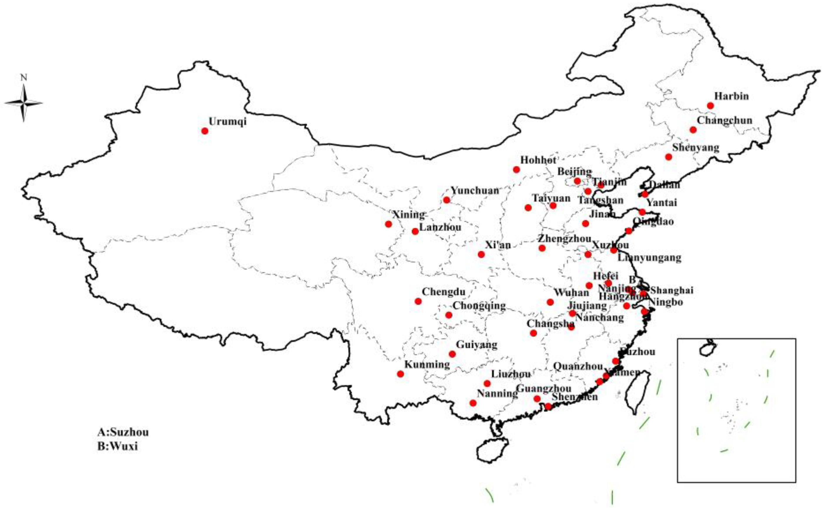
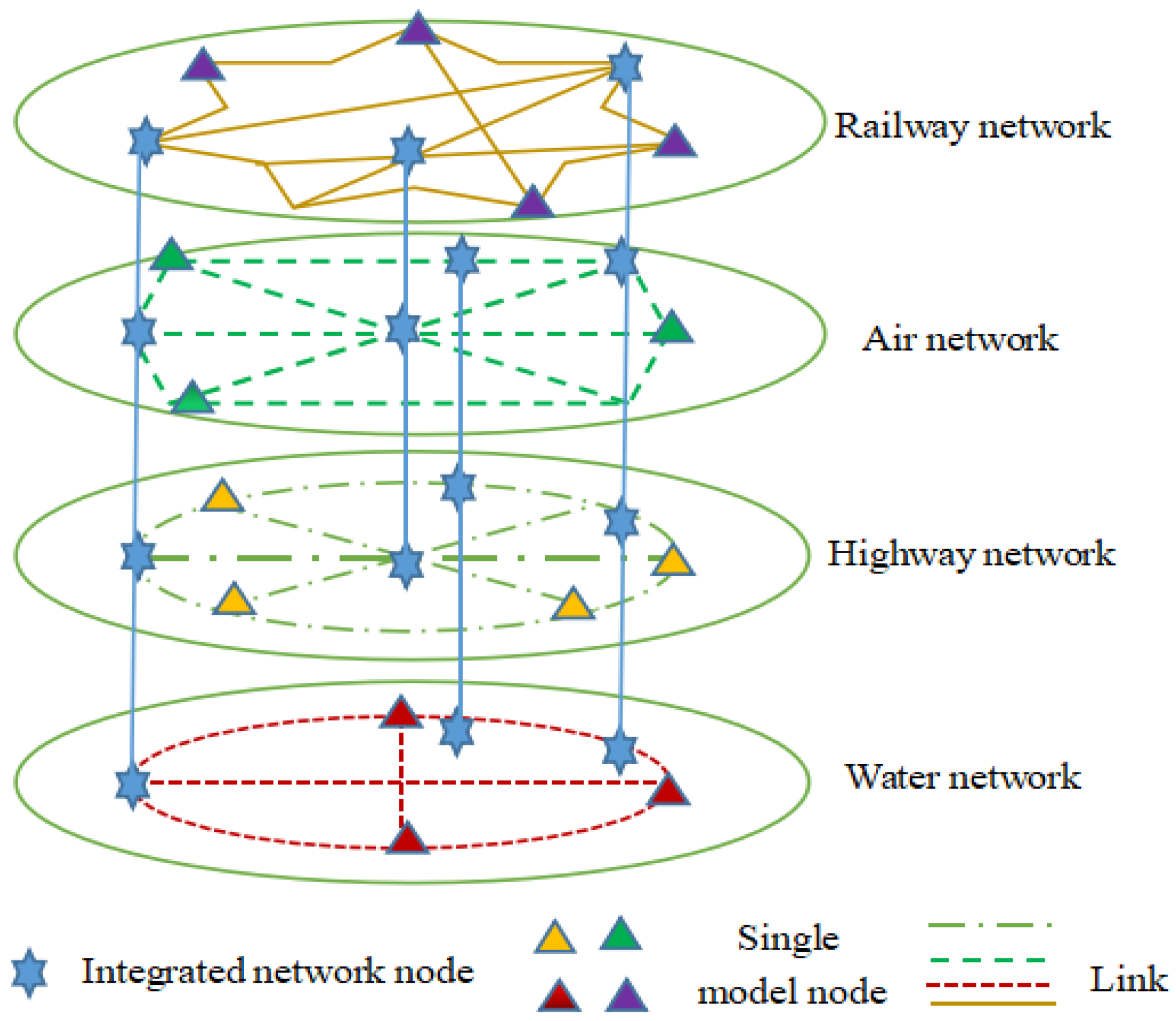
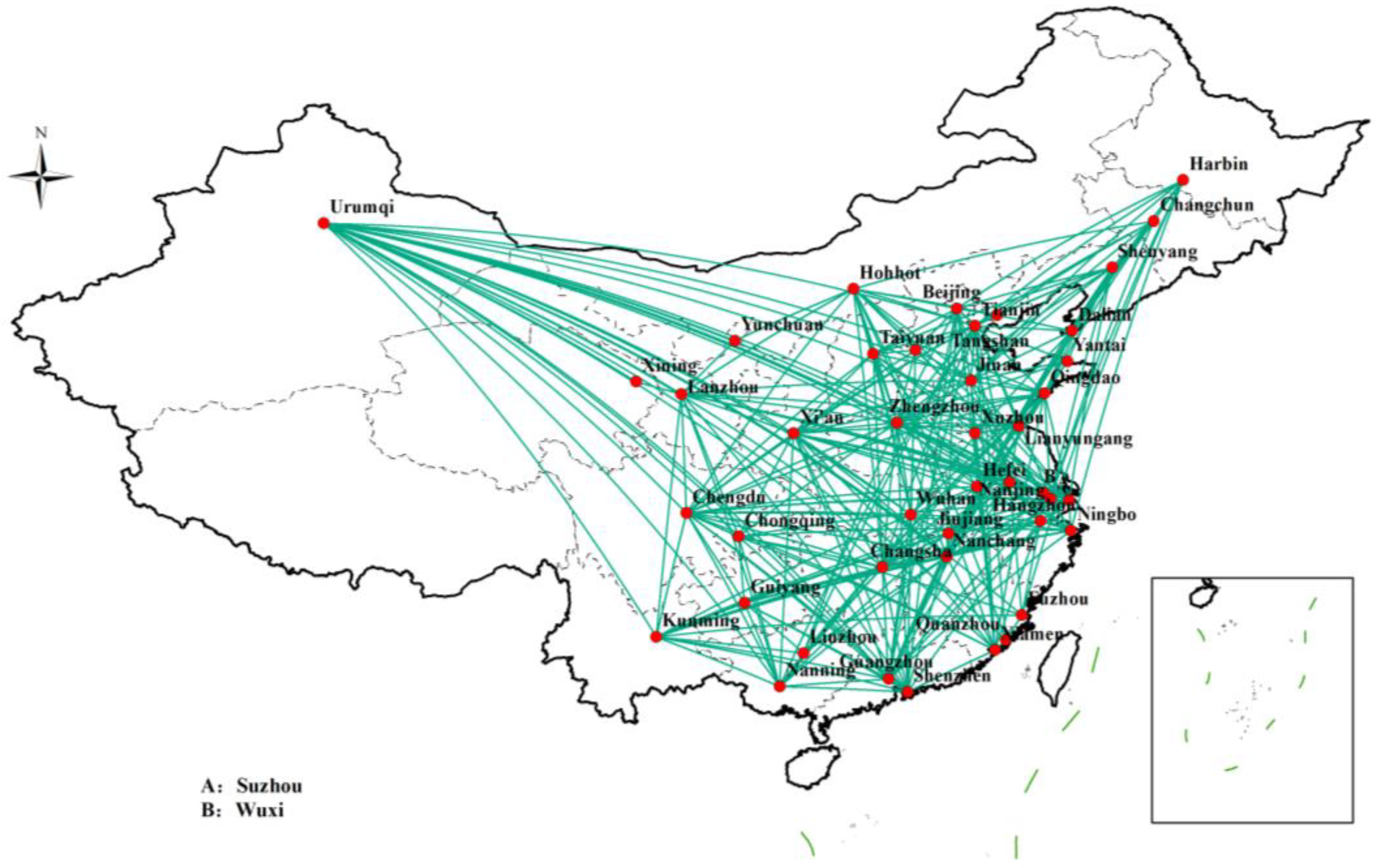
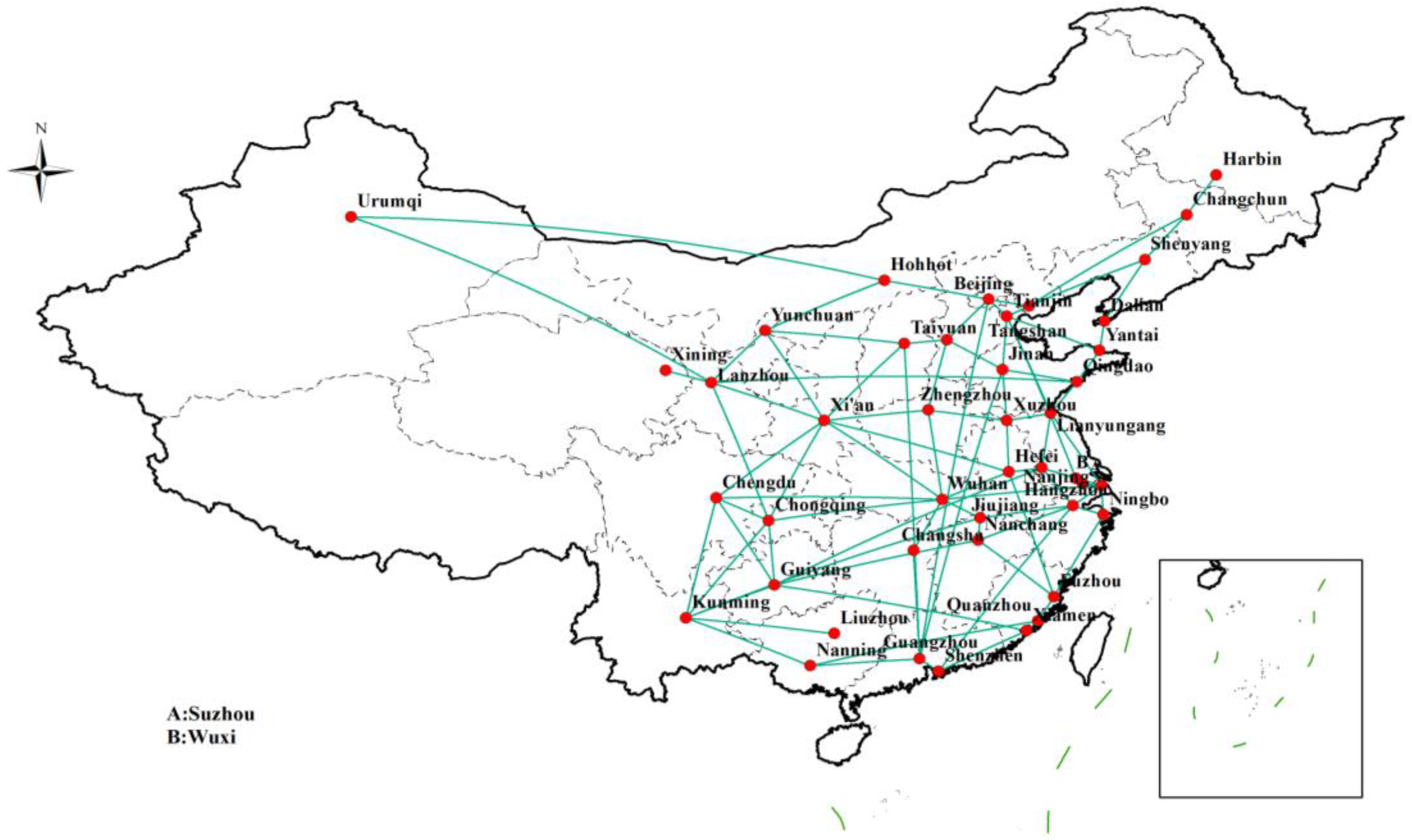


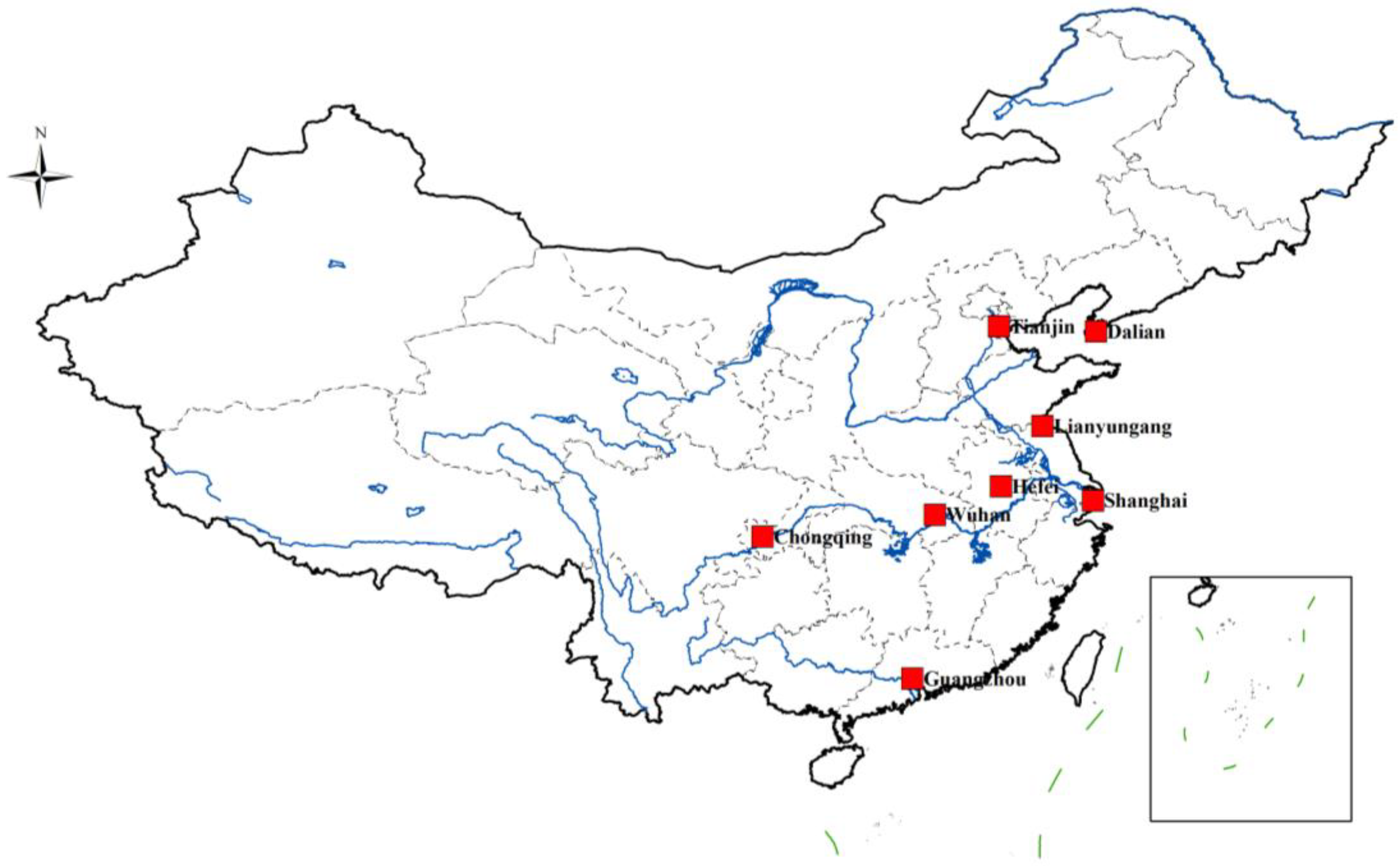
Disclaimer/Publisher’s Note: The statements, opinions and data contained in all publications are solely those of the individual author(s) and contributor(s) and not of MDPI and/or the editor(s). MDPI and/or the editor(s) disclaim responsibility for any injury to people or property resulting from any ideas, methods, instructions or products referred to in the content. |
© 2024 by the authors. Licensee MDPI, Basel, Switzerland. This article is an open access article distributed under the terms and conditions of the Creative Commons Attribution (CC BY) license (https://creativecommons.org/licenses/by/4.0/).