Seismic Stability Study of Bedding Slope Based on a Pseudo-Dynamic Method and Its Numerical Validation

Abstract

Earthquakes are one of the main causes of bedding slope instability, and scientifically and quantitively evaluating seismic stability is of great significance for preventing landslide disasters. This study aims to assess the bedding slope stability under seismic loading and the influences of various parameters on stability using a pseudo-dynamic method. Based on the limit equilibrium theory, a general solution for the dynamic safety factor of bedding slope is proposed. The effects of parameters such as slope height, slope angle, cohesion, internal friction angle, vibration time, shear wave velocity, seismic acceleration coefficient, and amplification factor on stability are discussed in detail. To evaluate the validity of the pseudo-dynamic solution, the safety factors are compared with those given by early cases, and the results show that the safety factors calculated by the present formulation coincide better with those of previous methods. Moreover, a two-dimensional numerical solution of bedding slope based on Mohr–Coulomb’s elastic–plastic failure criterion is also performed by using the finite element procedure, and the minimum safety factor is essentially consistent with the result of the pseudo-dynamic method. It is proved that the pseudo-dynamic method is effective for bedding slope stability analyses during earthquakes, and it can overcome the limitations of the pseudo-static method.

1. Introduction

Bedding slope is one of the most common types of slope in geological engineering and is more prone to instability during earthquakes. Once instability happens, it not only causes enormous casualties and damage, but also pollutes the surrounding geological environment [1,2]. Serious landsides even create huge geological hazards and result in a great amount of cost in repairs or rebuilding. Due to bedding slope existing widely in hydraulic engineering, highway engineering, construction engineering, railway engineering, etc., its stability evaluation is one of the urgent problems in practical engineering. Consequently, the study of the dynamic characteristics and stability of bedding slope under seismic loading is of great importance for understanding the mechanisms of disasters and preventing landslide disasters [3,4].

Unit now, the safety factor has been a crucial parameter for seismic slope stability, and its solutions mainly include the limit equilibrium theory and the finite element technique. Since the 20th century, a large number of domestic and foreign scholars have conducted extensive studies on the seismic slope stability problem and proposed various calculated methods. Among these methods, the pseudo-static method is a typical analysis approach for seismic slope stability and is also a dominant approach in various standards. This pioneering work of the pseudo-static method was first reported by Terzaghi [5], which later became the most common method for assessing seismic slope stability. In this approach, the acceleration generated by earthquake shaking is considered to produce seismic inertia force. The advantage of this approach is that it can define the seismic force as a constant without taking into account the variation in time and space. Then, the safety factor of the slope is computed by using the limit equilibrium theory, but the result is a little conservative. Seed [6] provided a suggested value of the seismic acceleration coefficient and discussed the stability of earth dams by comparison with the displacement data. Since then, with the development of soil mechanics theory, the pseudo-static method has been widely and successfully used in many areas. In the past four decades, many scholars, such as Bray et al., Siyahi et al., Ausilio et al., Deng et al., Karray et al., and Ye et al., also applied this approach to study the seismic stability of reinforced slope, consolidated slope, layered slope, and multistage loess slope [7,8,9,10,11,12]. Although the pseudo-static method is widely used in theoretical analysis and practical application because of its uncomplicated format, the results obtained are conservative and not realistic compared with the previous study.

To overcome the drawback of the pseudo-static approach, a pseudo-dynamic approach was proposed by Steedman et al. [13], and the rationality of this method was proved by Bash et al. [14]. This approach not only considers the influence of variation time and phase difference during earthquakes, but also the effect of the amplification factor through soil. Because of its potential advantages, Choudhury et al. [15] introduced a calculation method for soil pressure behind retaining walls that considers both horizontal and vertical seismic accelerations simultaneously, which further perfects the pseudo-dynamic theory. Later, Choudhury et al. [16] also applied this approach to analyze the seismic stability of tailing dams and expanded its application. Recently, Lu et al. [17] used a pseudo-dynamic method to research the stability of sandy slopes in the framework of planar failure mechanism under complex conditions, and they gave a law of the safety factor with time. Zhou et al. [18,19] performed the pseudo-dynamic approach combined with the finite element upper bound method to assess seismic slope stability, and they discussed the influences of various parameters on stability. Kokane et al. [20] employed a modified pseudo-dynamic method to study the seismic stability of nailed vertical cut, and a closed-form solution was derived to estimate the influence of the seismic inertial force. For non-homogeneous slopes, Suman et al. [21] conducted a new pseudo-dynamic method to analyze a two-layered cohesive-friction soil slope, and the result was verified against finite element analysis. However, the pseudo-dynamic method was born with many congenital deficiencies, and an obvious one isthat the slip body is defined as a rigid body. This means that the deformation of the slope cannot be obtained in the whole process of earthquake. Therefore, the slope stability can only be explained by the single safety factor when applying the pseudo-dynamic method.

The other calculation method for the safety factor, the finite element numerical method, which analyzes the failure mechanism between the structural plane and slip body in its entirety, is often conducted using commercial software [22]. Owing to consideration of the effects of the slope elastic–plastic deformation, this approach has the advantages of reasonably simulating the complex seismic dynamic process and interaction mechanics between the slip body and surrounding rock mass. In the finite element method, the slope stability problem can assume a plane strain condition in Mohr–Coulomb’s strength theory. Hence, many researchers provided a variety of finite element methods and their analysis methods have been different from each other since the 1940s [23]. Matsui et al. [24] developed a shear strength reduction technique for slope stability analysis based on the finite element technique, and the centerpiece of that study was that the slope failure was defined according to the shear strain failure criterion. Zheng et al. [25] discussed the computation method for the safety factor and location of the critical slip surface in finite element slope stability in detail under the strength reduction framework, and the effectiveness of the proposed procedures were demonstrated by an actual case. Moreover, for definitions of the safety factor, including the strength reserving definition and overloading definition, Zheng et al. [26] provided some strategies for how to select the safety factor for different slope types when the finite element method was used for the slope stability analysis. In recent years, Qin et al. [27] carried out the finite element lower bound and finite element upper bound approach to analyze the seismic stability of soil slope with the weak interlayer, and they determined the safety factor upper or lower limit. Karthik et al. [28] analyzed the influences of constitutive models such as the Mohr–Coulomb model and hardening soil model on slope stability by using the numerical simulation technique, and the results showed that the Mohr–Coulomb model was better suited for stability analysis of slope due to the concise input parameters. Liu et al. [29] used the elastic finite element stress fields to analyze the slope stability, and a 2D rock slope problem involving a nonlinear failure model and a 3D shallow slope problem were adopted to validate the proposed method. Tomáš et al. [30] introduced a surface layer method for slope stability based on the finite element technique, which aimed to stabilize the surface of the calculation model in the strength reduction approach, and they verified it by the 2D and 3D slope problems. The studies mentioned above are important references to determine the slope safety factor. Although there are many advantages for the finite element technique, an unavoidable problem is that professional numerical software is usually needed to analyze the more complex numerical model, and it takes a long time to calculate the safety factor.

A quick and efficient approach to assess slope stability is often the center of attention for engineers. Therefore, in the present study, a pseudo-dynamic analysis model is proposed to consider the influences of seismic action on the stability of the bedding slope, in which the seismic acceleration is assumed to be a harmonic sinusoidal acceleration. A general solution of the safety factor with time is obtained by the limit equilibrium method, and the effects of various parameters such as slope parameters and seismic dynamic parameters on the stability of bedding slopes are discussed in detail. To verify the analytical results obtained from the present study, the safety factors are compared with the results of two early examples, and also a numerical model is developed by using the finite element technique to identify the critical slip surface and transient safety factor of a bedding slope. This present study provides an efficient and practical approach to assess the seismic dynamic characteristics and stability of the bedding slope under seismic loads. Furthermore, this method can also be combined with the permanent displacement method to evaluate the slope safety, and it has wide potential applications.

2. Pseudo-Dynamic Analysis Method of Bedding Slope Stability

2.1. Pseudo-Dynamic Method

At present, the pseudo-dynamic method is a comparatively common method, which can effectively simulate the input of seismic acceleration. Since the input is a harmonic sinusoidal acceleration, it not only simulates most of the characteristics of the seismic wave, but also simplifies the processing of calculation. Also, the seismic accelerations are assumed to be linear with slope depth from the top of the slope, so it is suitable for analytic solution. The variation of horizontal and vertical sinusoidal acceleration at any depth z below the top of the slope and time t with rock mass amplification factor f can be expressed as follows [13]:

$$\left\{\begin{array}{l}{a}_{\mathrm{h}}(z,t)=\left[1+\frac{H-z}{H}(f-1)\right]k_{\mathrm{h}}g\sin \left[\omega (t-\frac{H-z}{v_{\mathrm{s}}})\right]\\ a_{\mathrm{v}}(z,t)=\left[1+\frac{H-z}{H}(f-1)\right]k_{\mathrm{v}}g\sin \left[\omega (t-\frac{H-z}{v_{\mathrm{p}}})\right]\end{array}\right.$$

(1)

where a_h(z, t) and a_v(z, t) are the harmonic seismic waves of the horizontal and vertical seismic acceleration, respectively. v_s and v_p are the shear wave and primary wave velocities propagating through the rock mass, respectively. k_h and k_v are the horizontal and vertical seismic acceleration coefficients, respectively. ω is the angular frequency of the base shaking, which can be defined as ω = 2π/T, and T is the period of lateral and vertical shaking, which are assumed to have the same value in the analysis. f is the rock mass amplification factor, which represents a linear increase in the amplitudes of both horizontal and vertical acceleration from the base to the slope crest surface. H is the slope height. G is the shear modulus of rock mass, and g is the gravity acceleration. Similar to previous studies, the shear modulus is also considered as a constant with depth through the rock mass.

Under seismic load, the shear wave velocity v_s and primary wave velocity v_p with finite values through a bedding slope can be expressed as follows [31]:

$$\left\{\begin{array}{l}{v}_{\mathrm{s}}=\sqrt{\frac{G}{\rho }}\\ v_{\mathrm{p}}=\sqrt{\frac{G(2-2\mu )}{\rho (1-2\mu )}}\end{array}\right.$$

(2)

where μ is Poisson’s ratio and ρ is the density of rock mass.

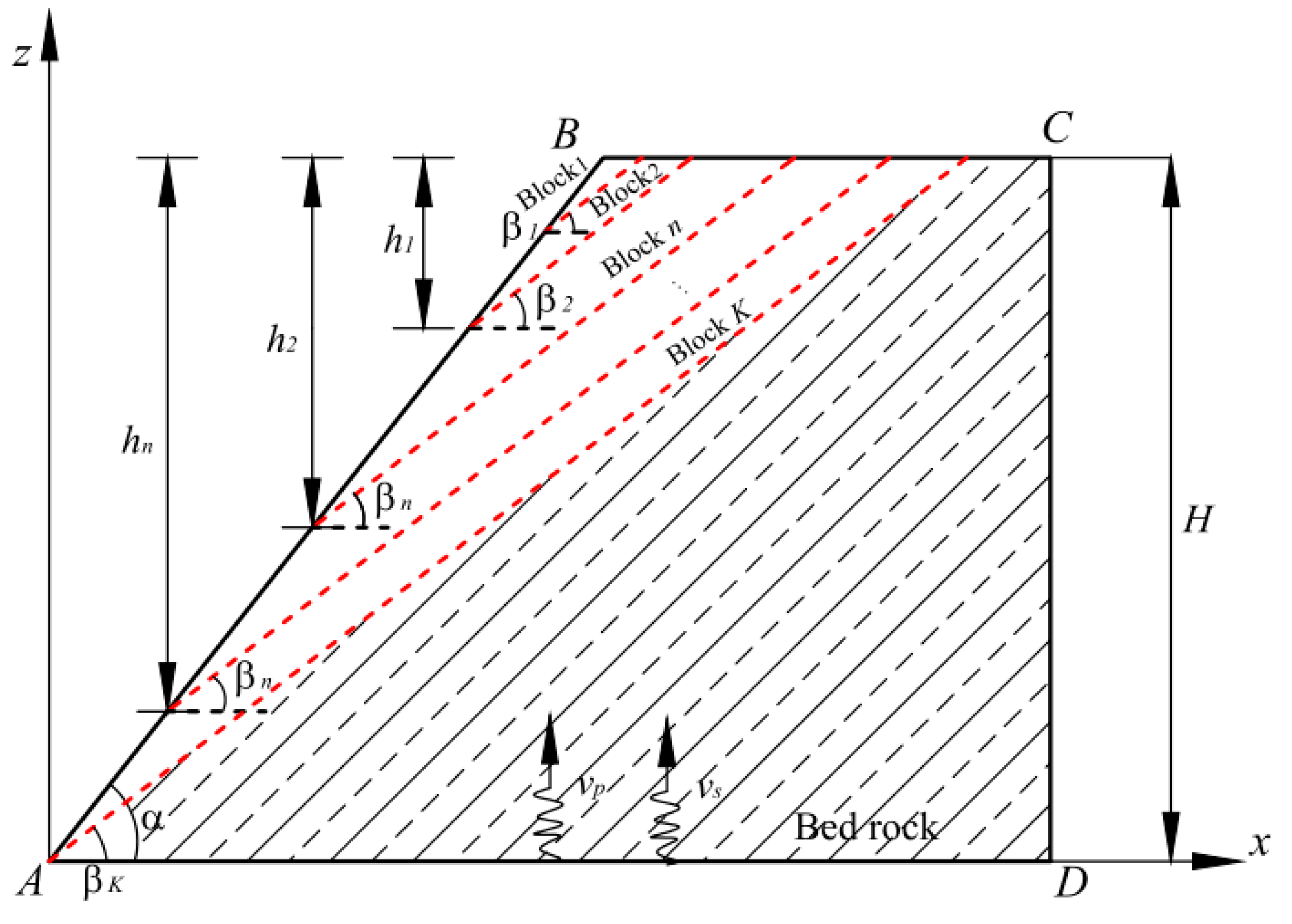
2.2. Simplified Mechanical Model

Failure of the bedding rock slope is the main type of slope instability. In geotechnical engineering, one of the most common viewpoints is that the structural plane is considered a potential slip surface. Thus, it can be assumed that the slip surface of the bedding slope is a plane and the slip block sliding may occur at various structural planes. Figure 1 is a typical generalized model of bedding slope. In Figure 1, a total of K structural planes is considered with each dip angle of β_i, and the slope angle is α. The rock mass between adjacent structural planes is named Block_i, the height of each block from the top of the slope is h_i, and the length of the slip surface is l_i. The red dotted lines represent structural planes. A general geometric model of the bedding slope is established under the Cartesian coordinate system and the coordinate origin at the location of the slope toe A (0, 0).

In mathematics, the face of the slope can be expressed as

$$z=\tan \alpha x$$

(3)

Then, the equation of each structural plane is given by

$$z=\tan {\beta }_{i}x+b_i$$

(4)

where

$$b_i=\left(H-h_i\right)\left(1-\frac{\tan {\beta }_i}{\tan \alpha }\right)$$

The relationship between h_i and l_i can be expressed as

$$\frac{h_i}{l_i}=\cos \left(\frac{\pi }{2}-{\beta }_i\right)$$

(5)

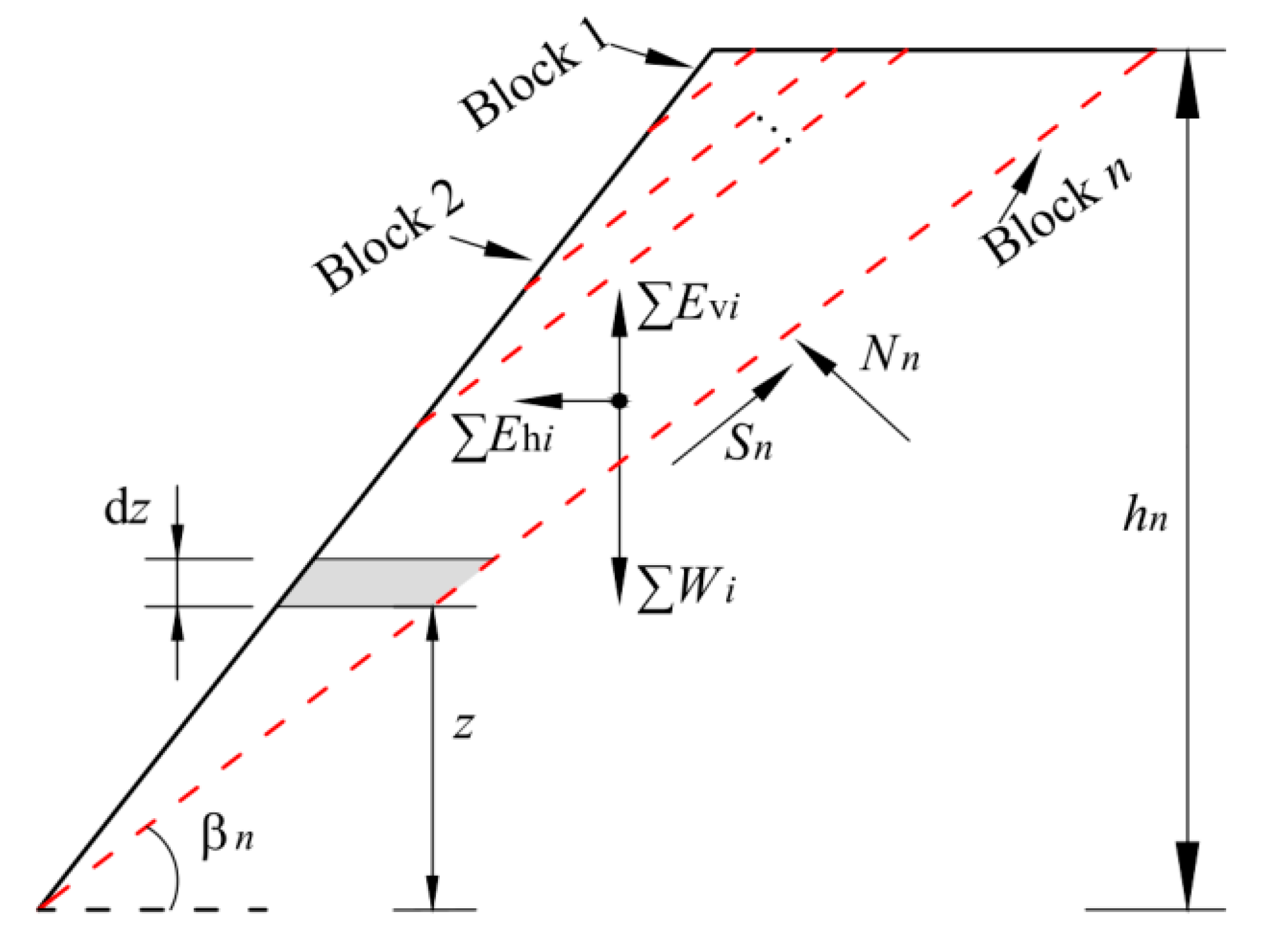
2.3. Determination of Forces of Slip Block

This calculated model is considered as a set of rigid bodies, and each slip block does not produce deformation during the calculation process. Additionally, the seismic wave inputs are at the bottom of the calculated model, which is the same as the actual working conditions. Based on the above calculation principle, assuming that the structural plane i is a slip surface, the analytical model of the slip body is shown in Figure 2. The details of the calculation parameters are as follows: S_n and N_n are the tangential and normal forces on the structural plane n, respectively. W_i is the weight of the slip block i, and E_hi and E_vi are the horizontal and vertical seismic inertia forces of the slip block i, respectively. ${\displaystyle \sum _{i=1}^n{W}_i}$, ${\displaystyle \sum _{i=1}^n{E}_{\mathrm{h}i}}$, ${\displaystyle \sum _{i=1}^n{E}_{\mathrm{v}i}}$ are the total weight, the total horizontal seismic inertia forces, and the total vertical seismic inertia forces above the structural plane i, respectively.

2.3.1. Determination of Weight Force of Slip Block

For an arbitrary thin element of thickness dz at depth z, as shown in Figure 2, combining Equations (3) and (4), the mass of element can be described as

$$\mathrm{d}m\left(z\right)=\frac{\gamma }{g}\left[\left(z-b_i\right)\cot {\beta }_i-z\cot \alpha \right]\mathrm{d}z$$

(6)

where γ is rock mass unit weight. So, the weight of the whole slip body is given by

$$\begin{array}{l}{\displaystyle \sum _i^n{W}_i}={\displaystyle {\int }_{H-h_n}^{H}g\mathrm{d}m\left(z\right)}\\ ={\displaystyle {\int }_{H-h_n}^H\gamma \left[\left(z-b_n\right)\cot {\beta }_n-z\cot \alpha \right]\mathrm{d}z}\\ =\frac{\gamma }{2}\left(\cot {\beta }_n-\cot \alpha \right)\left[H^2-{\left(H-h_n\right)}^2\right]-\gamma b_n\cot {\beta }_n{h}_n\end{array}$$

(7)

where n is the serial number of the structural plane.

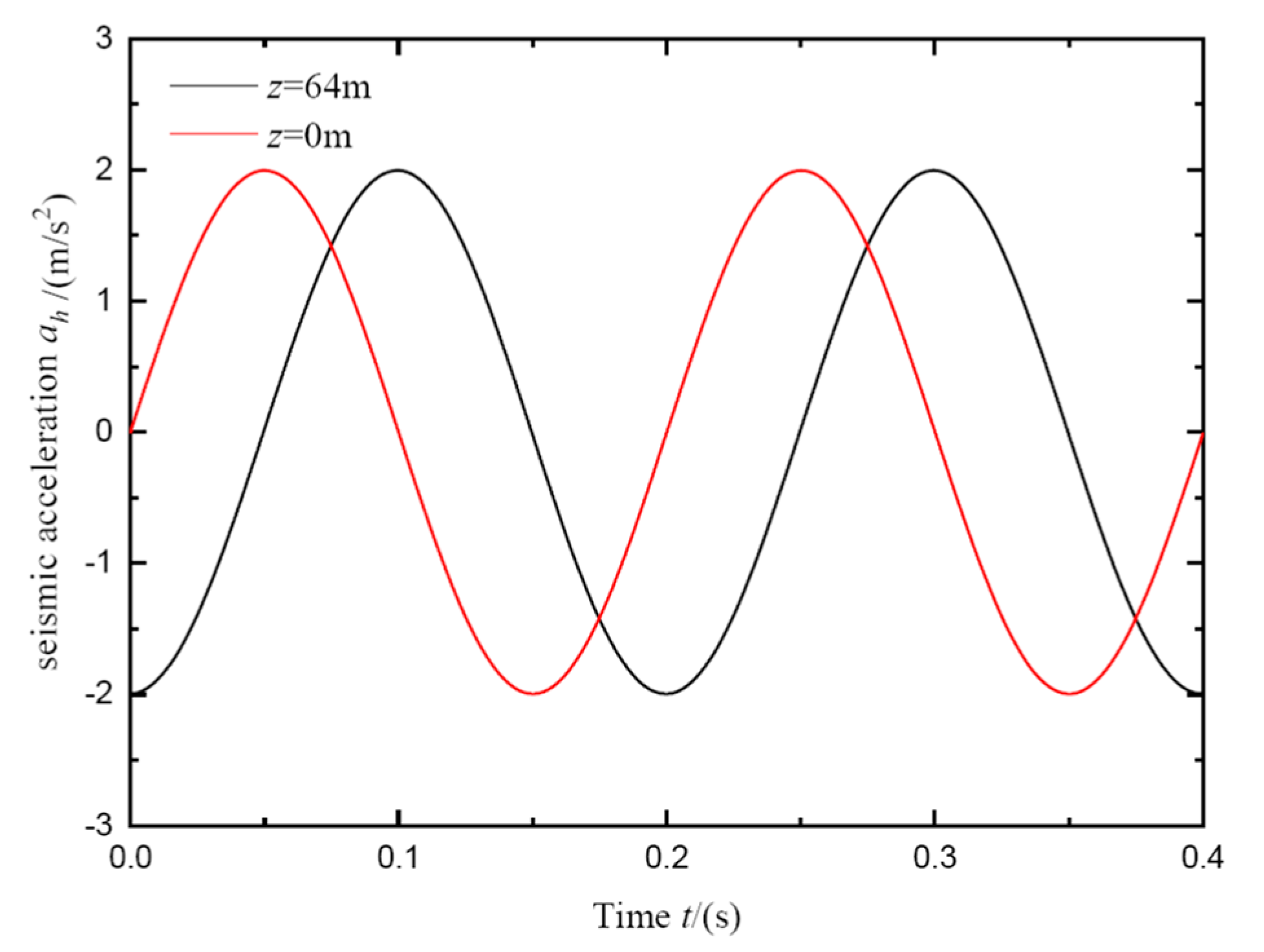
2.3.2. Determination of Horizontal Seismic Inertia Force of Slip Block

In the present study, the coordinate origin of the calculated model is located at the toe of the slope, as shown in Figure 1. It is important to note that the free surface at the top of the slope is defined as the coordinate origin in the pseudo-dynamic method, thus the value of z needs to be converted with the transformation of coordinate in Figure 2. To sum up, the total horizontal seismic forces of the whole slip body can be written as

$$\begin{array}{l}{\displaystyle \sum _i^n{E}_{\mathrm{h}i}}={\displaystyle {\int }_{H-h_n}^H{a}_{\mathrm{h}}\left(z,t\right)\mathrm{d}m\left(z\right)}\\ ={\displaystyle {\int }_{H-h_n}^H\left\{\gamma \left[\left(z-b_n\right)\cot {\beta }_n-z\cot \alpha \right]\left[1+\frac{z}{H}(f-1)\right]k_{\mathrm{h}}\sin \left[\omega (t-\frac{z}{v_{\mathrm{s}}})\right]\right\}\mathrm{d}z}\\ =\gamma k_{\mathrm{h}}\left\{\begin{array}{l}{m}_1\sin \left[\omega \left(t-\frac{H}{v_{\mathrm{s}}}\right)\right]+m_2\sin \left[\omega \left(t-\frac{H-h_n}{v_{\mathrm{s}}}\right)\right]\\ +m_3\cos \left[\omega \left(t-\frac{H-h_n}{v_{\mathrm{s}}}\right)\right]+m_4\cos \left[\omega \left(t-\frac{H}{v_{\mathrm{s}}}\right)\right]\end{array}\right\}\end{array}$$

(8)

where the coefficients m₁~m₄ can be expressed as follows:

$$\left\{\begin{array}{l}{m}_1=\left(\cot {\beta }_n-\cot \alpha \right)\frac{v_{\mathrm{s}}^2}{{\omega }^2}+\frac{f-1}{H}\left[\left(2H-b_n\right)\cot {\beta }_n-2H\cot \alpha \right]\frac{v_{\mathrm{s}}^2}{{\omega }^2}\\ m_2=-\left(\cot {\beta }_n-\cot \alpha \right)\frac{v_{\mathrm{s}}^2}{{\omega }^2}-\frac{f-1}{H}\left\{\left[2\left(H-h_n\right)-b_n\right]\cot {\beta }_n-2\left(H-h_n\right)\cot \alpha \right\}\frac{v_{\mathrm{s}}^2}{{\omega }^2}\\ m_3=-\left(\cot {\beta }_n-\cot \alpha \right)\left(H-h_n\right)\frac{v_{\mathrm{s}}}{\omega }+b_n\cot {\beta }_n\frac{v_{\mathrm{s}}}{\omega }+2\frac{f-1}{H}\left(\cot {\beta }_n-\cot \alpha \right)\frac{v_{\mathrm{s}}^3}{{\omega }^3}\\ -\frac{f-1}{H}\left\{\left[{\left(H-h_n\right)}^2-\left(H-h_n\right)b_n\right]\cot {\beta }_n-{\left(H-h_n\right)}^2\cot \alpha \right\}\frac{v_{\mathrm{s}}}{\omega }\\ m_4=\left(\cot {\beta }_n-\cot \alpha \right)H\frac{v_{\mathrm{s}}}{\omega }-b_n\cot {\beta }_n\frac{v_{\mathrm{s}}}{\omega }+\frac{f-1}{H}\left[\left(H^2-H{b}_n\right)\cot {\beta }_n-H^2\cot \alpha \right]\frac{v_{\mathrm{s}}}{\omega }\\ -2\frac{f-1}{H}\left(\cot {\beta }_n-\cot \alpha \right)\frac{v_{\mathrm{s}}^3}{{\omega }^3}\end{array}\right.$$

Similarly, the total vertical seismic forces of the whole slip body can be written as

$$\begin{array}{l}{\displaystyle \sum _i^n{E}_{\mathrm{v}i}}={\displaystyle {\int }_{H-h_n}^H{a}_{\mathrm{v}}\left(z,t\right)\mathrm{d}m\left(z\right)}\\ ={\displaystyle {\int }_{H-h_n}^H\left\{\gamma \left[\left(z-b_n\right)\cot {\beta }_n-z\cot \alpha \right]\left[1+\frac{z}{H}(f-1)\right]k_{\mathrm{v}}\sin \left[\omega (t-\frac{z}{v_{\mathrm{p}}})\right]\right\}\mathrm{d}z}\\ =\gamma k_{\mathrm{v}}\left\{\begin{array}{l}{m}_5\sin \left[\omega \left(t-\frac{H}{v_{\mathrm{p}}}\right)\right]+m_6\sin \left[\omega \left(t-\frac{H-h_n}{v_{\mathrm{p}}}\right)\right]\\ +m_7\cos \left[\omega \left(t-\frac{H-h_n}{v_{\mathrm{p}}}\right)\right]+m_8\cos \left[\omega \left(t-\frac{H}{v_{\mathrm{p}}}\right)\right]\end{array}\right\}\end{array}$$

(9)

where the coefficients m₅~m₈ can be expressed as follows:

$$\left\{\begin{array}{l}{m}_5=\left(\cot {\beta }_n-\cot \alpha \right)\frac{v_{\mathrm{p}}^2}{{\omega }^2}+\frac{f-1}{H}\left[\left(2H-b_n\right)\cot {\beta }_n-2H\cot \alpha \right]\frac{v_{\mathrm{p}}^2}{{\omega }^2}\\ m_6=-\left(\cot {\beta }_n-\cot \alpha \right)\frac{v_{\mathrm{p}}^2}{{\omega }^2}-\frac{f-1}{H}\left\{\left[2\left(H-h_n\right)-b_n\right]\cot {\beta }_n-2\left(H-h_n\right)\cot \alpha \right\}\frac{v_{\mathrm{p}}^2}{{\omega }^2}\\ m_7=-\left(\cot {\beta }_n-\cot \alpha \right)\left(H-h_n\right)\frac{v_{\mathrm{p}}}{\omega }+b_n\cot {\beta }_n\frac{v_{\mathrm{p}}}{\omega }+2\frac{f-1}{H}\left(\cot {\beta }_n-\cot \alpha \right)\frac{v_{\mathrm{p}}^3}{{\omega }^3}\\ -\frac{f-1}{H}\left\{\left[{\left(H-h_n\right)}^2-\left(H-h_n\right)b_n\right]\cot {\beta }_n-{\left(H-h_n\right)}^2\cot \alpha \right\}\frac{v_{\mathrm{p}}}{\omega }\\ m_8=\left(\cot {\beta }_n-\cot \alpha \right)H\frac{v_{\mathrm{p}}}{\omega }-b_n\cot {\beta }_n\frac{v_{\mathrm{p}}}{\omega }+\frac{f-1}{H}\left[\left(H^2-H{b}_n\right)\cot {\beta }_n-H^2\cot \alpha \right]\frac{v_{\mathrm{p}}}{\omega }\\ -2\frac{f-1}{H}\left(\cot {\beta }_n-\cot \alpha \right)\frac{v_{\mathrm{p}}^3}{{\omega }^3}\end{array}\right.$$

It is noticeable that a special case of the seismic inertia forces is given, in the limits, as follows:

$$\begin{array}{l}\underset{v_{\mathrm{s}}\to \infty }{\lim }{\left({\displaystyle \sum _i^n{E}_{\mathrm{h}i}}\right)}_{\max }={\left\{\sin \left(\omega t\right)k_{\mathrm{h}}{\displaystyle {\int }_{H-h_n}^H\gamma \left[\left(z-b_n\right)\cot {\beta }_n-z\cot \alpha \right]\mathrm{d}z}\right\}}_{\max }\\ =k_{\mathrm{h}}{\displaystyle \sum _i^n{W}_i}\end{array}$$

(10)

$$\begin{array}{l}\underset{v_{\mathrm{p}}\to \infty }{\lim }{\left({\displaystyle \sum _i^n{E}_{\mathrm{v}i}}\right)}_{\max }={\left\{\sin \left(\omega t\right)k_{\mathrm{v}}{\displaystyle {\int }_{H-h_n}^H\gamma \left[\left(z-b_n\right)\cot {\beta }_n-z\cot \alpha \right]\mathrm{d}z}\right\}}_{\max }\\ =k_{\mathrm{v}}{\displaystyle \sum _i^n{W}_i}\end{array}$$

(11)

The seismic inertia forces in the pseudo-dynamic method can be found to be equivalent to the results of the pseudo-static method when f = 1, v_s → ∞ and v_p → ∞, implying that the extreme value of the pseudo-dynamic method is the pseudo-static solution. Thus, the pseudo-static method is just a special case of the pseudo-dynamic method. As it should be, this also implicitly means that the safety factor obtained through the pseudo-static method will be slightly small.

2.4. Safety Factor Calculation of Bedding Slope

Under the limit equilibrium approach, the safety factor of a bedding slope can be described by the ratio of resisting force and driving force on the slip surface according to the Mohr–Coulomb strength theory. In view of the research object of Figure 2, the equilibrium equation is established according to force distributions for the pseudo-dynamic analysis. The solution of the dynamic equilibrium equation of the normal direction of the slip surface is obtained as

$$N_n+{\displaystyle \sum _{i=1}^n{E}_{\mathrm{h}i}}\sin {\beta }_n-\left({\displaystyle \sum _{i=1}^{n}W}-{\displaystyle \sum _{i=1}^n{E}_{\mathrm{v}i}}\right)\cos {\beta }_n=0$$

(12)

Similarly, the solution of the dynamic equilibrium equation of the tangential direction of the slip surface is obtained as

$${\displaystyle \sum _{i=1}^n{E}_{\mathrm{h}i}}\cos {\beta }_n+({\displaystyle \sum _{i=1}^n{W}_i}-{\displaystyle \sum _{i=1}^n{E}_{\mathrm{v}i}})\sin {\beta }_n-S_n=0$$

(13)

Based on these equations, the normal force N_n and tangential force S_n on the structural plane n can be determined. Therefore, the safety factor of the pseudo-dynamic method can be derived as

$$\begin{array}{l}F=\frac{c_n{l}_n+N_n\tan {\phi }_n}{S_n}\\ =\frac{c_n{l}_n+\left[\left({\displaystyle \sum _{i=1}^n{W}_i}-{\displaystyle \sum _{i=1}^n{E}_{\mathrm{v}i}}\right)\cos {\beta }_n-{\displaystyle \sum _{i=1}^n{E}_{\mathrm{h}i}}\sin {\beta }_n\right]\tan {\phi }_n}{{\displaystyle \sum _{i=1}^n{E}_{\mathrm{h}i}}\cos {\beta }_n+\left({\displaystyle \sum _{i=1}^n{W}_i}-{\displaystyle \sum _{i=1}^n{E}_{\mathrm{v}i}}\right)\sin {\beta }_n}\end{array}$$

(14)

where c is the cohesion of the structural plane, and φ is the internal friction angle of the structural plane. l is the length of the slip surface, and the value is equal to the length of the structural plane.

From Equation (14), it can be seen that the safety factor calculated by using the pseudo-dynamic method changes as a non-linear function of time with a shape that depends on the input seismic waves. Thus, the dynamic safety factor distribution is nonlinear, and this is completely different from the results of the pseudo-static method. Also, a significant advantage of the present method is that an explicit solution to the dynamic safety factor is obtained through the simple procedure. This is useful for quickly evaluating the safety of slopes under seismic working conditions.

3. Results Analysis of Pseudo-Dynamic Method

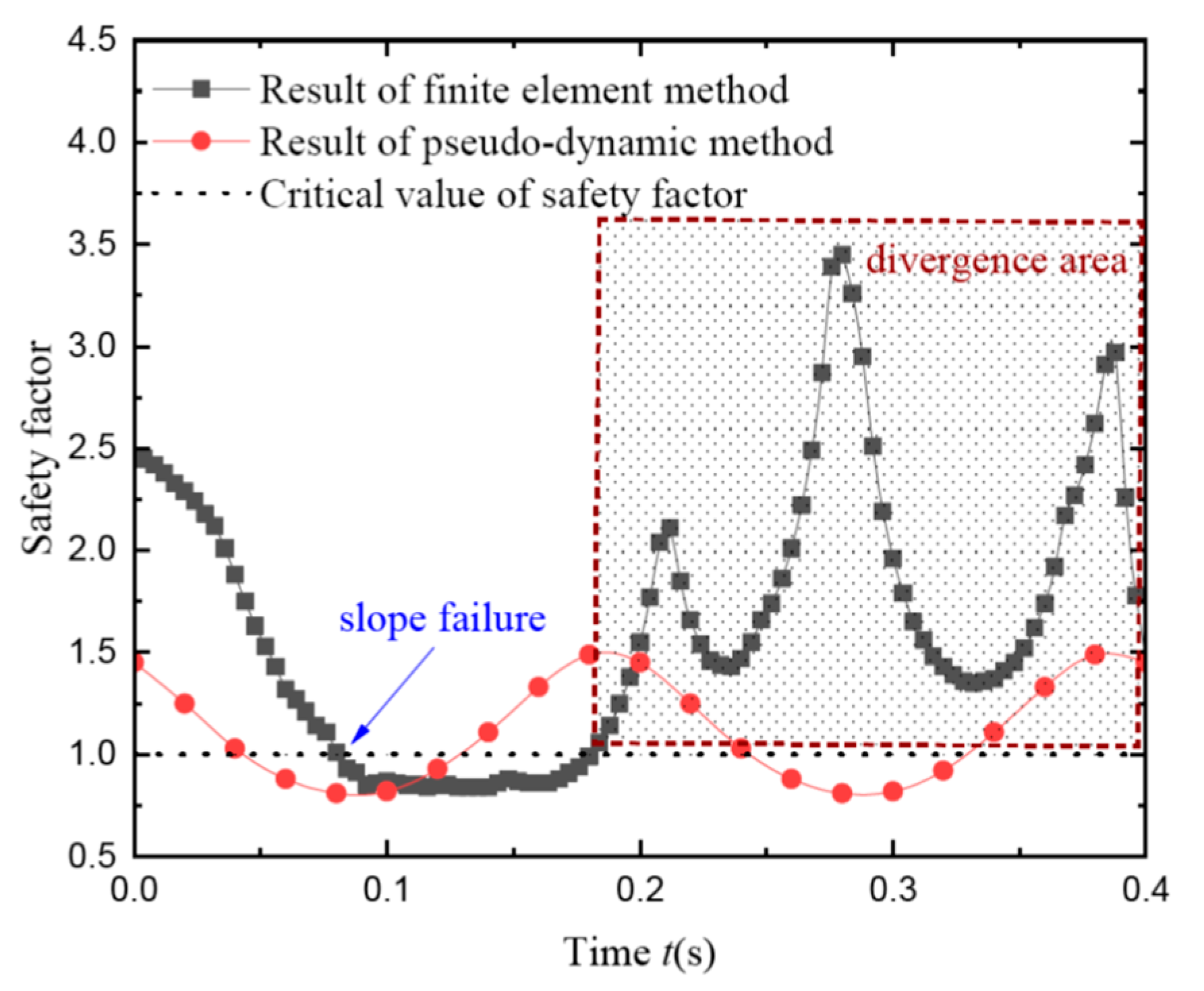
3.1. Validation of the Present Method

In order to verify the rationality of the pseudo-dynamic method, the safety factors of the two examples taken from the present method were compared with the results reported in Dong’s [32] studies based on different methods. One example was a comparison of slope safety that did not consider the seismic inertia force. Another example was a comparison of seismic slope safety using the pseudo-static method, the minimum stability factor method, and the dynamic analysis method.

Example 1.

The slope has height H = 60 m, slope angle is α = 60°, inclination of structural plane is β = 30°. The rock mass parameters are as follows: γ = 26.4 kN·m⁻³, c = 750 kPa, φ = 44.8°. The structural plane parameters are c = 150 kPa, φ = 28.8°. For Example 1, the stability of the slope is a static problem, without considering the seismic effect.

Table 1. Results for safety factor computed by different methods.

Result	Method
	Present	Simplified Janbu	Imbalance Thrust Force	Strength Reduction	Finite Element Slip Surface Stress
Safety factor	1.56	1.65	1.65	1.55	1.38
Error (%)	/	−5.45	−5.45	0.65	11.54

presents the safety factor calculated by different methods.

As can be seen from Table 1, the pseudo-dynamic method derived in this study provides a safety factor F that is in close agreement with the values obtained from the strength reduction method and is marginally less than the results of the simplified Janbu method and imbalance thrust force method. The present analytical result is satisfactory with the relative error between the calculated value and the reported values not exceeding 6%. It can be noted that the present result is slightly higher than the value calculated by the finite element slip surface stress method, and this significant difference can be attributed to the definition of the constitutive relation of rock mass and the selection of material parameters in the finite element method. Hence, under the framework of the limit equilibrium theory, the present result is reasonable compared with the other results and shows a good agreement.

Example 2.

The slope angle is α = 45°, inclination of structural plane is β = 27°, and height H = 64 m. The landslide translational slides along the structural plane, consisting of eluvial stone in the upper and pelitic siltstone and mudstone on the bottom. The landslide is located in the Sanjiang earthquake zone with the seismic region of VII degree fortification, and the horizontal seismic acceleration coefficient is k_h = 0.127. The eluvial stone parameters are as follows: γ = 19 kN·m⁻³, c = 9 kPa, φ = 34°. The siltstone parameters are γ = 23 kN·m⁻³, c = 245 kPa, φ = 47°.

If we only consider the effect of the seismic acceleration coefficient as a single factor on the slope stability, the present formulae may be reduced to the result of the pseudo-static method. It is observed from

Table 2. Results of the safety factor computed by different methods.

Result	Method
	Present	Pseudo-Static	Minimum Stability Factor	Dynamic Time-History Analysis
Safety factor	1.12	1.12	0.99	1.05
Error (%)	/	0	13.13	6.67

that the present result and the value obtained from the pseudo-static method matched exactly. As mentioned previously, the pseudo-static method is only a simple method to calculate the seismic effects. In fact, the pseudo-dynamic method is more rational because of the consideration of the variation of time and space. By comparing it to the minimum stability factor method and the dynamic analysis method, the similarities can be found which are that the finite element technique is used to calculate the safety factor. The consideration of the influence of the material elastic–plastic deformation results in a low safety factor being calculated with the above two methods. It is obvious that the results presented in Table 1 and Table 2 indicate that the present method is reasonable and effective.

3.2. Dynamic Characteristics of Bedding Slope

The slope contained one set of parallel structural planes, the inclination of the structural planes was β = 30°, and the spacing was 10 m. The height of the slope was H = 64 m and slope angle was α = 70°, as shown in Figure 3. The characteristics of the mechanical parameters of the slope rock masses are shown in

Table 3. Mechanical parameters of slope.

Material	Unit Weight γ (kN·m−3)	Elastic Modulus E/Pa	Poisson’s Ratio μ	Cohesion c/kPa	Internal Friction Angle φ/(°)
rock mass	25	1 × 1010	0.20	1000	38
structural plane	17	1 × 107	0.30	120	24

. The shear wave and primary wave velocity during earthquakes can be expressed as Equation (2); hence, the calculation parameters were as follows: v_s = 1290 m/s and 2106 m/s. The angular frequency ω can be calculated using the relation provided by Kramer, as T = 2π/ω = 4 H/v_s. Therefore, T = 0.2 s, ω = 31.4 rad/s. Table 3 represents the mechanical parameters of the slope.

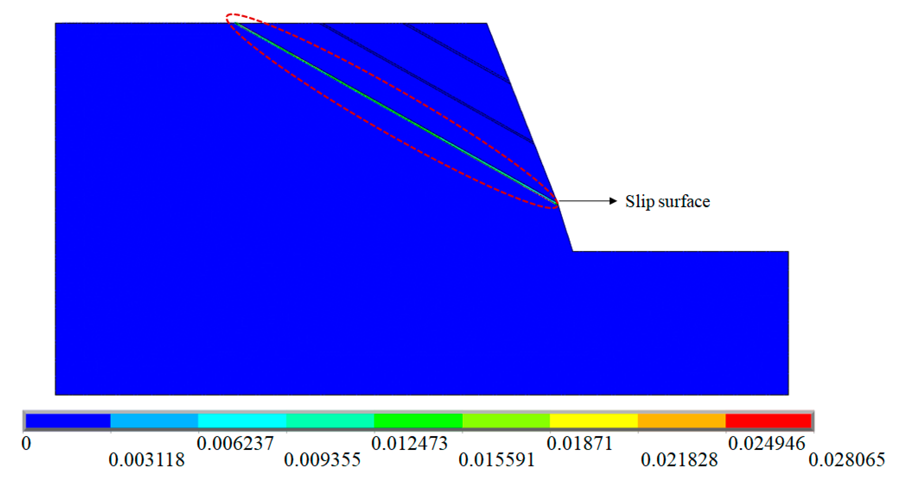
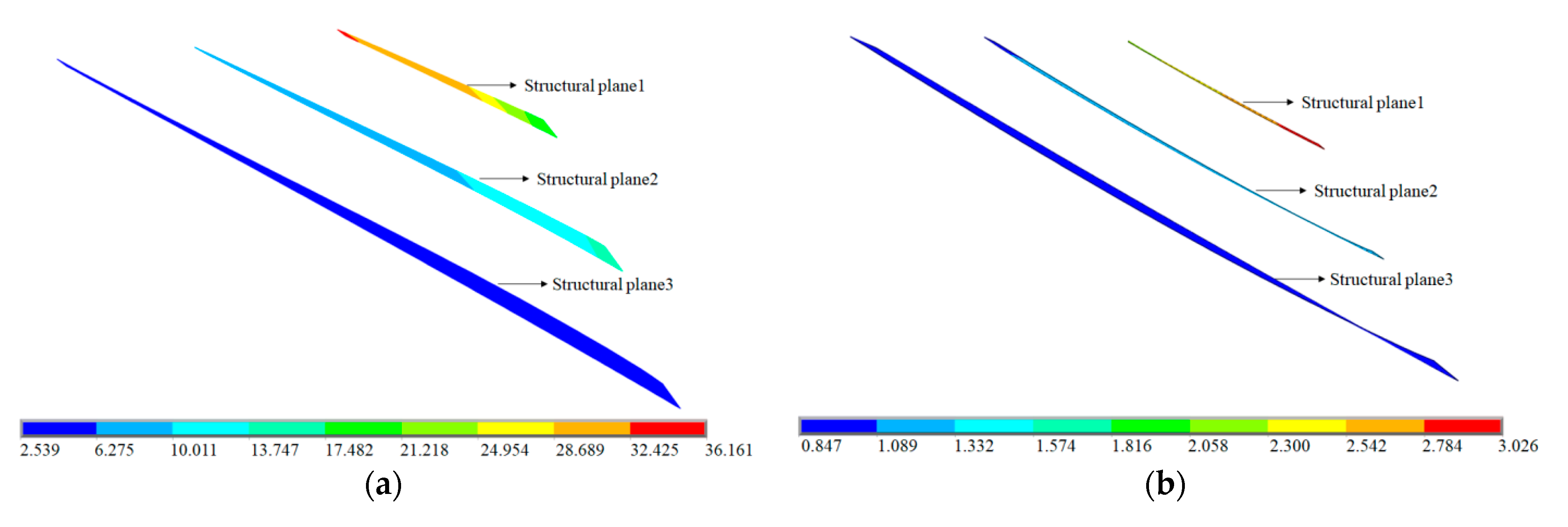
3.2.1. Determination of Slip Surface

Under the static force condition, the safety factor of different slip blocks was calculated by the present method, and the values were F₁ = 2.54, F₂ = 1.38, and F₃ = 1.07. As a result, the slip surface should be the structural plane closest to the slope toe, as shown in Figure 3. This conclusion is consistent with the results reported by Zhao et al. [33]. And that conclusion is based only on the results of the safety factor; if it is right, there will be an important complement for the field investigation of landslides.

3.2.2. The Effects of Various Parameters on Safety Factor

According to the concept of the dynamic safety factor, many factors influencing the safety factor are analyzed. These parameters can be divided into three categories in accordance with the attributes of influencing factors, such as dynamic parameters of the seismic action, geometrical parameters of the slope, and strength parameters of the slope. The following sections describe the influence of each parameter on the safety factor in more detail.

• The effects of dynamic parameters of the seismic action on safety factor

The dynamic parameters of the seismic action include computing time t, input wave velocity v_s, seismic acceleration coefficients k_h and k_v, and amplification factor f.

(1)

The effects of computing time t on safety factor

Unlike static working conditions, the seismic inertial force acting on the sliding body will cause the location of the slip surface to change over action time. Thus, it is necessary to search out the relationship between the safety factors, slip surface, and vibrating time. For the bedding slope, the structural plane is generally a potential slip surface because of the deterioration of the mechanical parameters of the rock mass. The rule of the safety factor of a set of structural planes with time can be obtained based on the pseudo-dynamic method, and every structural plane has one safety factor. The determination basis of the critical slip surface is based on the structural plane corresponding to the minimum safety factor. In this study, the evaluation standard for slope stability was the safety factor F ≥ 1, whether under static or dynamic working conditions. Thus, the safety factor of different slip bodies calculated by the pseudo-dynamic method can be seen in Figure 4.

In Figure 4, the dotted line represents the critical safety factor. Based on the results of Figure 4, the safety factor calculated by the pseudo-dynamic method changes with vibration time, which is not constant and is time-dependent. Obviously, the safety factor has periodic variational regularity and the curve of the safety factor is similar to that of the input wave from the pseudo-dynamic method. Considering that the safety factor is changing in the vibration process, selecting the minimum safety factor is used as a rule for stability evaluation, i.e., the dynamic safety factor. If the dynamic safety factor F < 1, the slope is instable. On the contrary, it is the opposite. Figure 4 shows that the safety factor of Blocks 1–3 is F = 0.81, which indicates sliding occurred in the slope. Therefore, it can be concluded that the location of the slip surface is the same whether under static or dynamic working conditions for the bedding slope; because of this location, it all corresponds to the minimum safety factor.

(2)

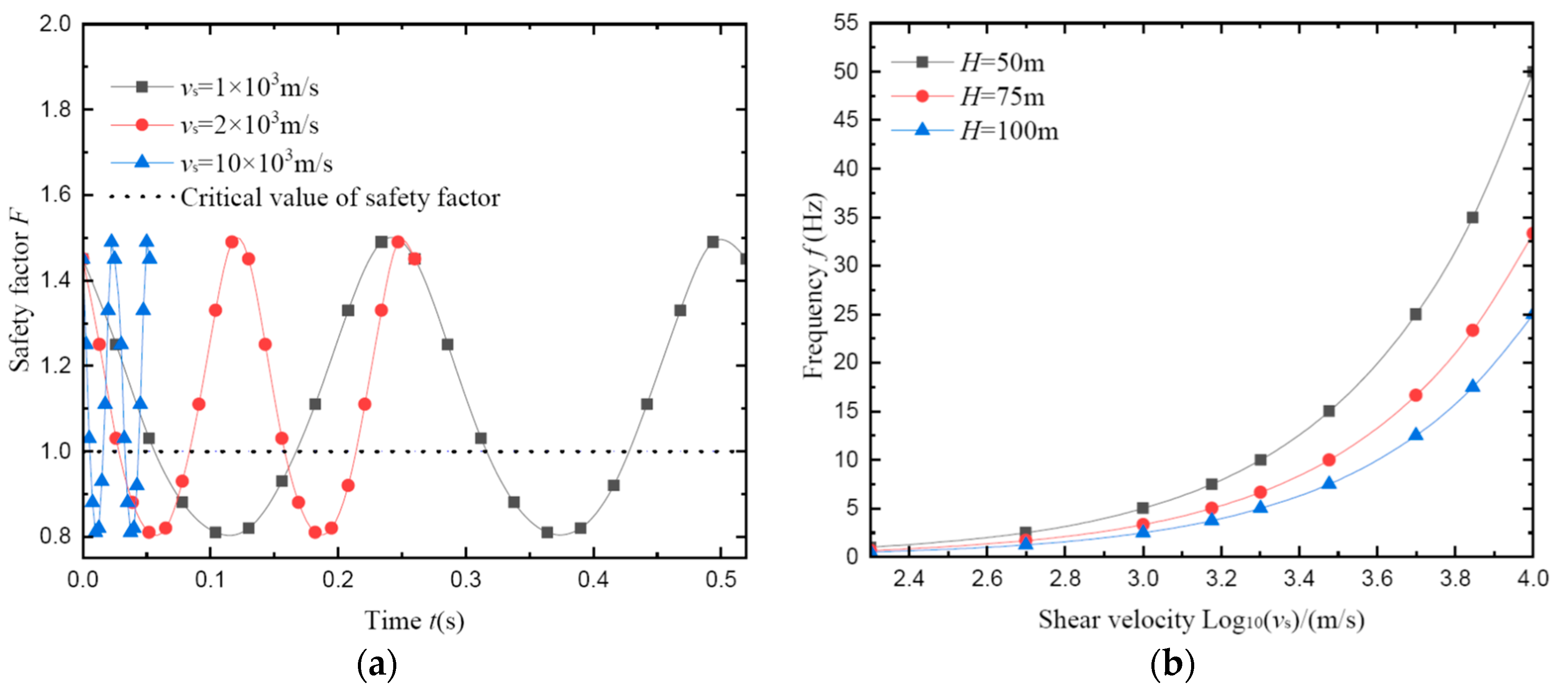
The effects of input wave velocity v_s on safety factor

The effects of shear wave velocity on the safety factor are depicted in Figure 5a. Therein, the shear velocity is 1 × 10³ m/s, 2 × 10³ m/s, and 10 × 10³ m/s, respectively. Interestingly, the maximum and minimum value of the dynamic safety factor under different velocities is the same, regardless of the input wave velocity. From Equation (1), it can be inferred that when the seismic acceleration coefficients are determined, the maximum input values are equivalent to the values of the pseudo-static method. Accordingly, the extreme values of the safety factors calculated by the two methods are also the same. However, the change frequency of the safety factor increases with the increase in the shear wave velocity, and this response frequency is highly sensitive to the change in velocity. From Figure 5a, for v_s = 1 × 10³~10 × 10³ m/s, the value of the frequency increases by 901.53% (from 3.9 Hz to 39.06 Hz). It will exacerbate the risk of slope instability when considering that the rock mass is a deformable material.

In order to better present the results, when the input wave velocity changes from 500 m/s to 10,000 m/s, for the slope heights H = 50 m, H = 75 m, and H = 100 m, the relationship between change frequency and input wave velocity is shown in Figure 5b. A Log₁₀ (v_s) value is employed as the abscissa because the range of the velocity is too large. The change frequency of the safety factor increases significantly with the increase in the shear wave velocity, especially for the lowest-height slope. In the present study, the rock mass was considered only as a rigid body based on the limit equilibrium theory, so the change frequency did not have an influence on the safety factor. However, in the deformation mechanism of rock mass, the change frequency will affect the deformation degree and morphology of rock mass, and thereby affect the dynamic stability of rock mass. Hence, this parameter is of great importance for slope deformation.

(3)

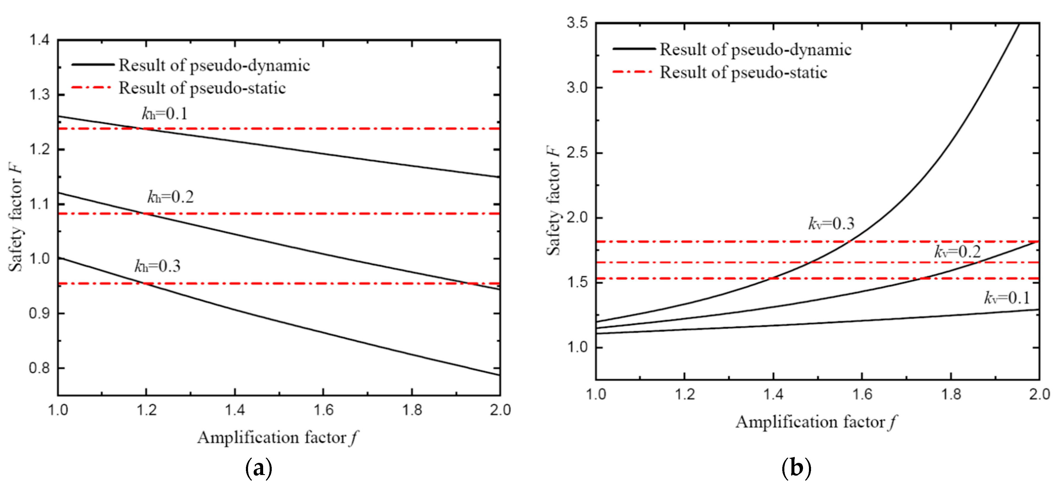
The effects of seismic acceleration coefficients k_h and k_v on safety factor

The effects of the horizontal and vertical seismic coefficients on the safety factor calculated by the present method were compared with the results of the pseudo-static method, and the results are shown in Figure 6. In the whole calculations, the range and values of the parameters were k_h = 0~0.4 and k_v = 0~0.4, respectively. Here, the effect of seismic combination was not considered in the analysis; only the seismic action in a single horizontal or vertical direction was considered. It can be seen that the results of the two methods have a discrepancy, mainly because the shear wave velocity v_s and v_p are limited. For Figure 6a, the safety factor calculated by the pseudo-dynamic method is smaller than that of the pseudo-static method. This can be explained by the seismic acceleration in the pseudo-dynamic method, in which the absolute value of the acceleration varies from 0 to k_hg, whereas the acceleration in the pseudo-static method is invariably a constant, i.e., k_hg. It is difficult for the seismic acceleration to converge to the maximum value, due to the value of v_s not being large enough in the pseudo-dynamic method. The smaller the input shear wave velocity, the greater the discrepancy in the results. Also, notice the directions of the seismic inertia forces associated with the calculated results and the differences between the two.

Additionally, from Figure 6, it can be seen that the seismic acceleration coefficients have a direct effect on the slope stability, and that the safety factor changes slightly nonlinearly with an increase in k_h or k_v. When k_h > 0, it represents a horizontal inertia force whose direction points to the outside of the slope, which means that the rock mass is more prone to cracking. During an earthquake, this adds the unfavorably oriented seismic inertia force to the slip body, which may cause slope instability. As shown in Figure 6a, the safety factor decreases with an increase in k_h, and this seismic inertia force of outside direction will seriously attenuate the slope stability. As an illustration, for φ = 40°, when k_h increases 0~0.4, the safety factor decreases by 40.16% (from 1.9 to 1.14). Similarly, when k_v > 0, it represents a vertical inertia force whose direction points to the outside of the slope, which means that the driving force of the rock mass will decrease. This is logical since a greater k_v implies a weaker driving force to which a slope is subject, thereby improving slope safety. As shown in Figure 6b, the safety factor increases with an increase in k_v. For example, for φ = 40°, when k_v increases 0~0.4, the safety factor increases by 15.78% (from 1.9 to 2.2). As can be seen in Figure 6a, the effect of k_v on the safety factor is lower than that of k_h, and less than half.

In order to better understand the law of the safety factor with the k_h and k_v, the spatial distribution of safety factors under the bidirectional seismic interaction is depicted in Figure 7. In Figure 7, the colors in different positions indicate the values of the safety factor under different horizontal and vertical seismic action, with red representing the high value and blue representing the low value. It can be seen that the influence efficiency of k_h on the safety factor is significantly greater than k_v, so the horizontal inertia force plays a vitally important role in the instability of the bedding slope under seismic loads. And that, fundamentally, is why vertical seismic acceleration is often ignored in the simplified analysis process, and only horizontal seismic acceleration is considered. However, for some important slope engineering in the high-intensity seismic belt, it is necessary to consider the effects of vertical seismic action because the earthquake itself has multi-dimensional characteristics. Additionally, more and more, the destruction phenomena after earthquakes show that considering the effects of vertical seismic action in slope stability analysis is becoming increasingly important.

(4)

The effects of amplification factor f on safety factor

Figure 8 represents the effects of the amplification factor on the safety factor. It can be seen that the amplification factor also has an important influence on slope stability; as f increases, the difference in the results between the pseudo-dynamic method and the pseudo-static method also increases, especially for the higher values of f. According to a comparative study of the two methods, the results of the pseudo-dynamic method are gradually increasing (k_v = 0.1~0.3) or decreasing (k_h = 0.1~0.3) with f increasing, whereas the results of the pseudo-static method are unchanged. Note that when the amplification factor changes, the degree of influence on the safety factor caused by seismic acceleration coefficients in the vertical direction is obviously larger than that in the horizontal direction. For example, when k_v = 0.3, f increases from 1.0 to 2.0 and the value of the safety factor increases by 218.49% (from 1.19 to 3.19). However, for k_h = 0.3, the value of the safety factor decreases only by 21.78% (from 1.01 to 0.79). Thus, this shows that, when considering the background of the amplification factor, the vertical seismic acceleration coefficient still has a significant effect on slope stability. From the above analysis, based on the parameters of the seismic acceleration coefficient and amplification factor effects on the safety factor, it can be concluded that the pseudo-dynamic method is more reasonable for considering the seismic effect.

2.

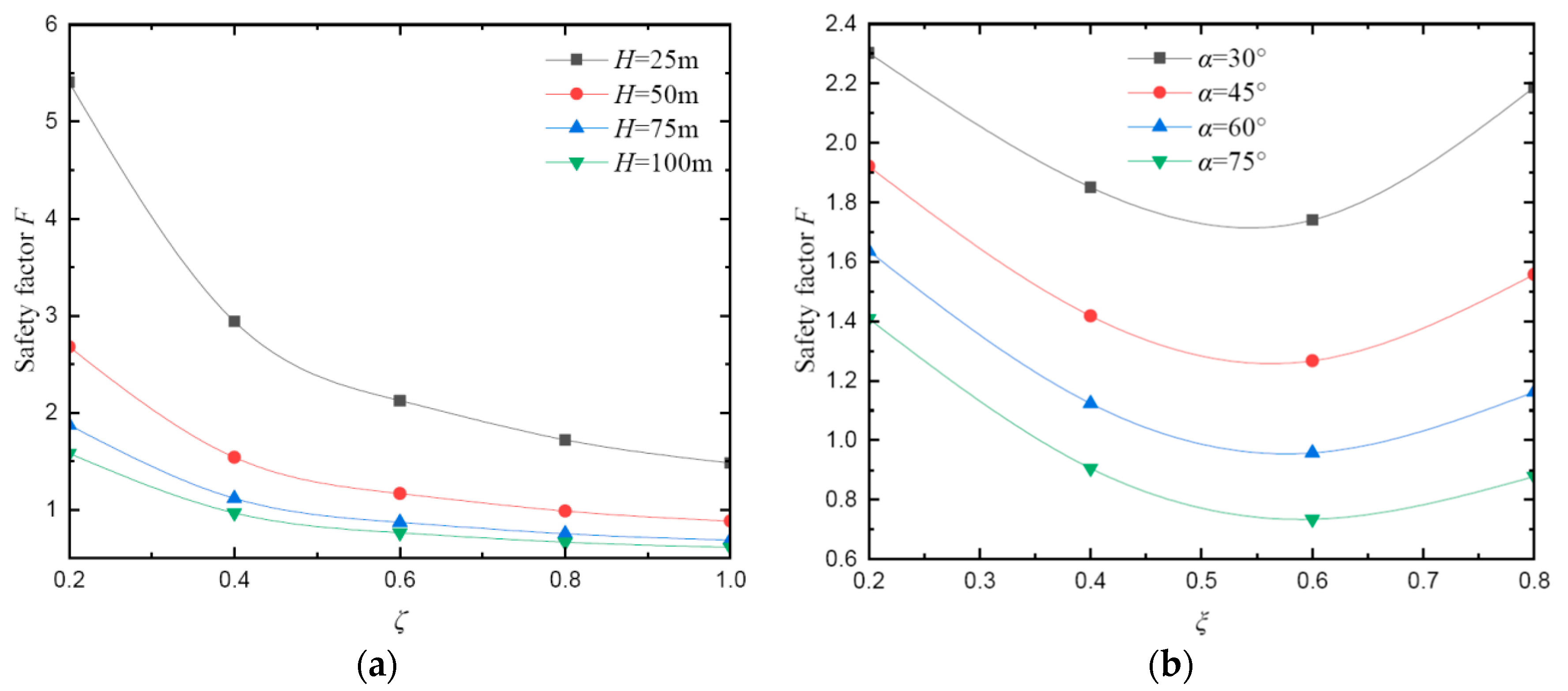
The effects ofgeometrical parameters of slope on safety factor

The geometrical parameters of slope mainly include slope height H and slope angle α. Figure 9 illustrates the effects of the slope height and slope angle on the safety factor. In this section, the varying ranges of these parameters are H = 25~100 m and α = 30°~75°, respectively, and two parameters ζ = h_i/H and ξ = β_i/α are defined to characterize the safety factor. It clearly seems that the safety factor decreases with the increase in both slope angle and slope height. From Figure 9a, it can be observed that the safety factor decreases as ζ increases, and when the slope height is higher, the value of the safety factor is lower. When ζ < 0.6, the attenuation gradient of the safety factor obviously has a relatively larger value, which means that the height of the slip body has a significant impact on the safety factor, especially when the slope height does not exceed 50 m, and vice versa. For example, for the slope heights H = 75 m and H = 100 m, when ζ increases from 0.6 to 1.0, the safety factor only decreases by 21.84% and 19.73%, respectively (from 0.87 to 0.68, and from 0.76 to 0.61). As shown in Figure 9b, the safety factor first decreases as ξ is increased and then increases as ξ is further increased. Interestingly, there is an optimal value for ξ that corresponds to the minimum safety factor, and that value is approximately ξ = 0.5~0.6. That result is of great importance in the initial evaluation safety of a bedding slope.

3.

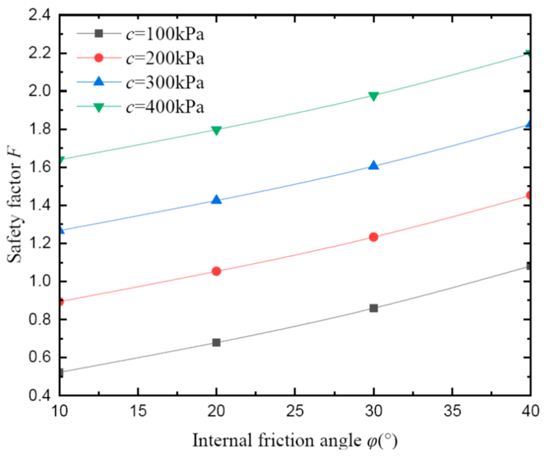
The effects of strength parameters of slope on safety factor

In geotechnical mechanics theory, the shear strength parameters of rock mass mainly include cohesion and internal friction angle. Thus, the influences of cohesion and internal friction angle on the safety factor are presented in Figure 10. Here, the varying ranges of the parameters were c = 100~400 kPa and φ = 10°~40°. It can be observed that the safety factor increases almost linearly with an increase in the internal friction angle and cohesion. In fact, the strength parameters of the structural planes are usually lower than for rock mass; this deterioration of the materials will seriously threaten the stability of the bedding slope due to inferior mechanics function. Obviously, the structural planes with higher values for the strength parameters are more likely to maintain the stability of the slope by inherent natural resistance. This result verifies the feasibility of enhancing the slope stability by using the anchor technology in bedding rock mass with a weak structural plane.

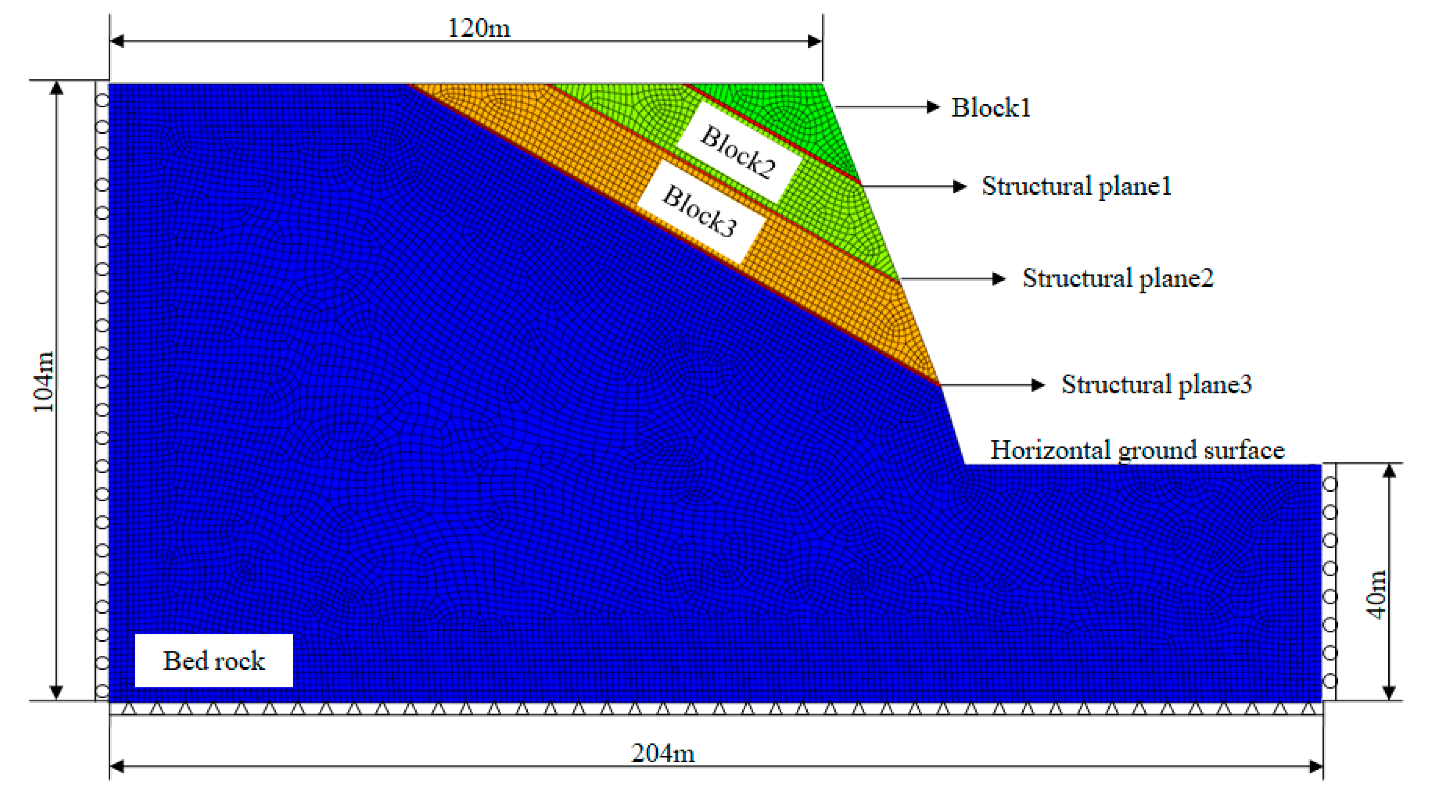
4. Numerical Analysis of Pseudo-Dynamic Method

In order to further verify the reliability of the pseudo-dynamic method, a two-dimensional finite element analysis of the bedding slope under the condition of an earthquake was performed by using ANSYS software. In the first phase, a stability analysis of this slope under static working conditions was performed by the elastic–plastic finite element strength reduction method, and the slip surface could be directly obtained. The finite element model is illustrated in Figure 11. In the numerical model, three thin weak layers were used to replace the structural planes above the horizontal ground surface, and the Mohr–Coulomb constitutive model simulated the failure behaviors and deformation of the rock mass. The calculated model considered plane strain and eight-node quadrilateral elements to determine the slip surface and safety factor. The boundary conditions in the calculation program were as follows: the bottom of the slope was set as a fully fixed constraint, and both sides of the model were set as horizontal fixed hinge support, and the other sides of the model were free, as shown in Figure 11.

Figure 12 shows the slip surface of the bedding slope obtained by the numerical simulation. The numbers on contours represent the equivalent plastic strain on the yield surface. It can be found that the plastic zone only runs through structural plane 3, so it is reasonable to determine that structural plane 3 is the slip surface and this result is consistent with the result from the pseudo-dynamic method under the static working conditions. Moreover, the safety factor calculated by the strength reduction method was F = 1.15, and this value was relatively close to the result of the pseudo-dynamic method F = 1.07, and the error was 7.48%.

In the second phase, seismic dynamic analysis of the bedding slope was performed. One typical sinusoidal acceleration wave used in this numerical analysis is shown in Figure 13. The seismic acceleration coefficient was set to k_h = 0.2, which was exactly the same value as in the previous pseudo-dynamic method.

In this phase, the result of the static analysis was regarded as the initial stress condition of the dynamic analysis, while the static boundary conditions were modified to artificial viscous–elastic boundaries. The advantage of this is that the artificial viscous–elastic boundaries can be applied to better simulate wave propagation at the boundary. The operation process in the numerical simulation was to apply the normal and tangential spring stiffness and damping coefficients at the boundary points. The normal and tangential spring stiffness can be expressed as follows [34]:

$$\left\{\begin{array}{l}{K}_{\mathrm{bn}}=\frac{1}{1+A}\frac{\lambda +2G}{2R}\\ K_{\mathrm{bt}}=\frac{1}{1+A}\frac{G}{2R}\end{array}\right.$$

(15)

where K_bn and K_bt are normal and tangential spring stiffness at the boundary points, respectively. G is the shear modulus of rock mass. R is the distance from the wave source to the viscous–elastic boundary point. A is the characteristic parameter of the input wave, A = 0.8. λ is the Lame coefficient, which can be expressed as

$$\lambda =\frac{2G\mu }{\left(1-2\mu \right)}$$

(16)

The normal and tangential damping coefficients can be expressed as follows:

$$\left\{\begin{array}{l}{C}_{\mathrm{bn}}=B\rho v_{\mathrm{p}}\\ C_{\mathrm{bt}}=B\rho v_{\mathrm{s}}\end{array}\right.$$

(17)

where C_bn and C_bt are normal and tangential damping coefficients, respectively. B is the characteristic parameter of the input wave, B = 1.1. v_s and v_p are the shear wave velocity and primary wave velocity, respectively. ρ is the density of rock mass.

In the numerical simulation, a point safety factor method was used to quantitatively analyze the bedding slope stability [35]. For this simulation, it took about 100 steps to calculate the seismic inertia force duration of 0.4 s, and the initial and final time steps were 0.004 s. Based on the Mohr–Coulomb constitutive model, the minimum point safety factor on the calculated element at any time of slope can be derived as

$$F_{\min (t)}=\frac{2\sqrt{\left(\tan \phi {\sigma }_1+c\right)\left(\tan \phi {\sigma }_3+c\right)}}{{\sigma }_1-{\sigma }_3}$$

(18)

where σ₁ and σ₃ are the maximum and minimum principal stress, respectively. c and φ are cohesion and internal friction angle of rock mass, respectively.

Figure 14 shows the safety factor contours of the structural plane at different times. Obviously, the safety factor of structural plane 3 was lower than the other two positions, and the value of the safety factor was F = 0.847 at the time of 0.1 s. This once again indicates that structural plane 3 was the slip surface.

For verifying the conclusion of the pseudo-dynamic method, the transient safety factor was compared between the numerical and analytical results, as shown in Figure 15. Firstly, it can be seen that before 0.1 s, the safety factors calculated by the different methods gradually decrease with time. The minimum safety factor of the numerical simulation was F = 0.847, which was close to the value of the pseudo-dynamic method F = 0.81. Therefore, both methods indicated that the bedding slope had been damaged. Secondly, the safety factor of the numerical method was almost unchanged at 0.1~0.2 s, but the result of the pseudo-dynamic method increased. The major reason for the difference is the essence of the calculated methods. The slip body is regarded as rigid in the pseudo-dynamic method, but a deformation body is adopted in the numerical calculation. Due to the feature that deformation is large before slope failure, the curve of the safety factor after instability will be divergent in the numerical result. Thirdly, although in general the numerical method obtained a slightly higher safety factor compared with the analytical data before 0.1 s, the evaluation standard for stability in this study was the minimum safety factor F ≥ 1, so the numerical results were in accordance with the conclusions of the pseudo-dynamic method.

5. Discussion

Under the principle of the minimum safety factor, a pseudo-dynamic method for evaluating bedding slope stability is proposed in this study. Although this approach is relatively simple and efficient compared with the pseudo-static approach and finite element technique, it also has some underlying problems worth discussing.

It is widely known that the structural plane of the bedding slope may be a potential slip surface, but this type of slope usually contains a group of structural planes. In a rigid body mechanics framework, the uniqueness of the slip surface can be determined by the principle of the minimum safety factor based on the limit equilibrium theory. However, the slip block and structural plane is an interaction relationship, and such interaction or mutual influence is going on in a synergetic and coupled manner considering that the slope is a deformable body during the dynamic action. In light of this, multi-slip surface failure may occur in bedding slopes under seismic load, and the pseudo-dynamic method in existence cannot yet be used to solve this question perfectly. Song et al. developed an extended Newmark sliding block model to investigate multi-slip seismic displacements of bedding rock slopes, and this method is considered as a supplement for the pseudo-dynamic method [2]. Therefore, the combined finite element technique with the pseudo-dynamic model should be developed and employed to analyze the seismic response and failure mode of bedding slopes, which will be key points for further research.

Moreover, the basis for determining the safety factor still needs to be carefully explored. Seed opined that a slope may also be stable even if the safety factor is less than 1, if the slope only produces a certain amount of cumulative displacement and deformation, which is not enough to cause slope failure [36]. The permanent displacement is another crucial parameter for seismic slope stability, but better links with the safety factor need to be built. Several researchers who have attempted to correlate the safety factor with displacement to overcome the shortcomings of the traditional limit equilibrium theory have not advanced very far and the results also need to be subjected to practical testing. Li et al. and Xiao et al. established a relationship between the safety factor and displacement based on the soil shear constitutive model and Morgenstern–Price assumption of interslice forces, and this has provided a foundation for the combination of the two evaluation parameters of slope stability [37,38]. Compared with the traditional safety method, the significant advantage of this technique is that it considers the influence of permanent displacement. In this study, the results of the pseudo-dynamic method show that the minimum safety factor converges to the result of the pseudo-static approach without considering the effect of the rock mass amplification factor, which may amplify the risk of slope instability. In order to better explain failure and assess the mechanisms of a slope, combining the safety factor and permanent displacement to evaluate the seismic stability of the slope will be a great point of exploration. The pseudo-dynamic approach is an effective analytic method offering a theoretical basis and feasible measurement for a dual-parameter stability evaluation.

6. Conclusions

The stability of bedding slopes is analyzed based on the pseudo-dynamic method in this study, and the influences of slope parameters and seismic parameters on stability are also investigated. The feasibility of the pseudo-dynamic method is verified by comparison with the results of earlier examples and the finite element method. To sum up, the following conclusions are obtained:

(1)

The slip surface of a bedding slope is the structural plane closest to the slope toe, and this conclusion has been confirmed by the pseudo-dynamic method and numerical simulation in this study. It has a great theoretical significance for understanding the slip mechanism of bedding slopes.

(2)

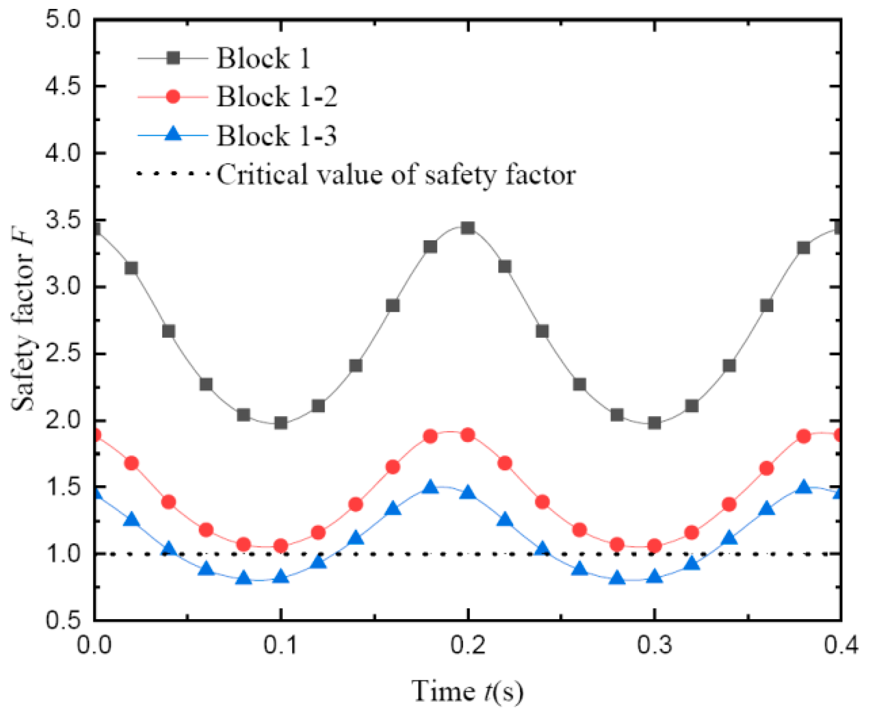
The safety factor obtained by the pseudo-dynamic method shows an apparent periodical characteristic with time. Hence, the minimum transient safety factor is defined as the dynamic safety factor under the seismic load. Without offering enough consideration of practical deformation, the pseudo-dynamic method makes the safety factor overly conservative.

(3)

The influences of slope parameters on the safety factor include both that the safety factor increases linearly with an increase in the internal friction angle and cohesion, but decreases with the increase in both slope angle and slope height; and that there seems to be an optimal value corresponding to the minimum safety factor for the structural plane angle and slope angle, and the ratio is approximately 0.5~0.6.

(4)

The influences of seismic parameters on the safety factor include the following: the influences of seismic acceleration coefficients on the safety factor are mainly shown by vibration time and direction, and the influence efficiency of k_h on the safety factor is significantly greater than k_v; the effect of the seismic amplification coefficient on the safety factor is different at different vibration times, and it can effectively simulate the seismic inertia force at different positions compared with the pseudo-static method; and the input wave velocity only affects the changing frequency of the safety factor, but has no effect on its extreme value.

References

1. Zhu, S.B.; Shi, Y.L.; Lu, M.; Xie, F.R. Dynamic mechanisms of earthquake-triggered landslides. Sci. China Earth Sci. 2013, 56, 1769–1779. [Google Scholar] [CrossRef]
2. Song, J.; Lu, Z.X.; Pan, Y.H.; Ji, J.; Gao, Y.F. Investigation of seismic displacements in bedding rock slopes by an extended Newmark sliding block model. Landslides 2023, 21, 461–477. [Google Scholar] [CrossRef]
3. Zang, M.D.; Yang, G.X.; Dong, J.Y.; Qi, S.W.; He, J.X.; Liang, N. Experimental study on seismic response and progressive failure characteristics of bedding rock slopes. J. Rock. Mech. Geotech. Eng. 2022, 14, 1394–1405. [Google Scholar] [CrossRef]
4. Cui, S.H.; Pei, X.J.; Yang, H.L.; Zhu, L.; Jiang, Y.; Zhu, C.; Jiang, T.; Huang, R.Q. Bedding slope damage accumulation induced by multiple earthquakes. Soil Dyn. Earthq. Eng. 2023, 173, 108175. [Google Scholar] [CrossRef]
5. Terzaghi, K.; Peek, R.B. Soil Mechanics in Engineering Practice; John Wile: New York, NY, USA, 1948. [Google Scholar]
6. Seed, H.B. Considerations in the earthquake-resistant design of earth and rockfill dams. Geotechnique 1979, 29, 215–263. [Google Scholar] [CrossRef]
7. Bray, J.D.; Repetto, P.C. Seismic design considerations for lined solid waste landfills. Geotext. Geomembr. 1994, 13, 497–518. [Google Scholar] [CrossRef]
8. Shyahi, B.G. Pseudo-static stability analysis in normally consolidated soil slopes subjected to earthquake. Tek. Dergi/Tech. J. Turk. Chamb. Civ. Eng. 1998, 9, 457–461. [Google Scholar]
9. Ausilio, E.; Conte, E.; Dente, G. Seismic stability analysis of reinforced slopes. Soil Dyn. Earthq. Eng. 2000, 19, 159–172. [Google Scholar] [CrossRef]
10. Deng, D.P.; Li, L.; Zhao, L.H. Research on quasi-static method of slope stability analysis during earthquake. J. Cent. South Univ. 2014, 45, 3578–3588. [Google Scholar]
11. Karray, M.; Hussien, M.N.; Delisle, M.C.; Ledoux, C. Framework to assess pseudo-static approach for seismic stability of clayey slopes. Can. Geotech. J. 2018, 55, 1860–1878. [Google Scholar] [CrossRef]
12. Ye, S.H.; Zhang, R.H. Stability analysis of multistage loess slope under earthquake action based on the pseudo-static method. Soil Mech. Found. Eng. 2023, 60, 304–313. [Google Scholar] [CrossRef]
13. Steedman, R.S.; Zeng, X. The influence of phase on the calculated of pseudo-static earth pressure on a retaining wall. Geotechnique 1990, 40, 103–112. [Google Scholar] [CrossRef]
14. Basha, B.M.; Babu, G.L.S. Seismic rotational displacements of gravity walls by pseudo dynamic method with curved rupture surface. Int. J. Geomech. 2010, 10, 93–105. [Google Scholar] [CrossRef]
15. Choudhuary, D.; Nimbalkar, S. Pseudo-dynamic approach of seismic active earth pressure behind retaining wall. Geotech. Geol. Eng. 2006, 24, 1103–1113. [Google Scholar] [CrossRef]
16. Choudhuary, D.; Nimbalkar, S. Seismic stability of tailings dam by using pseudo-dynamic method. In Proceedings of the ICSMGE—The 17th International Conference on Soil Mechanics and Geotechnical Engineering, Alexandria, Egypt, 5–9 October 2009; IOS Press: Amsterdam, The Netherlands, 2009; pp. 1542–1545. [Google Scholar]
17. Lu, Y.L.; Chen, X.R.; Wang, L. Analytical computation of sand slope stability under the groundwater seepage and earthquake conditions. Adv. Civ. Eng. 2022, 2022, 5286878. [Google Scholar]
18. Zhou, J.F.; Qin, C.B. Finite-element upper-bound analysis of seismic slope stability considering pseudo-dynamic approach. Comput. Geotech. 2020, 122, 103530. [Google Scholar] [CrossRef]
19. Zhou, J.F.; Zheng, Z.Y.; Bao, T.; Tu, B.X.; Yu, J.; Qin, C.B. Assessment of rigorous solutions for pseudo-dynamic slope stability: Finite-element limit-analysis modelling. J. Cent. South Univ. 2023, 30, 2374–2391. [Google Scholar] [CrossRef]
20. Kokane, A.K.; Sawant, V.A.; Sahoo, J.P. Seismic stability analysis of nailed vertical cut using modified pseudo-dynamic method. Soil Dyn. Earthq. Eng. 2020, 137, 106294. [Google Scholar] [CrossRef]
21. Suman, H.; Sima, G.; Richi, P.S. New pseudo-dynamic analysis of two-layered cohesive-friction soil slope and its numerical validation. Front. Struct. Civ. Eng. 2020, 14, 1492–1508. [Google Scholar]
22. Griffiths, D.V.; Lane, P.A. Slope stability analysis by finite elements. Geotechnique 1999, 49, 387–403. [Google Scholar] [CrossRef]
23. Duncan, J.M. State of the art: Limit equilibrium and finite-element analysis of slopes. J. Geotech. Geoenviron. Eng. 1996, 122, 577–596. [Google Scholar] [CrossRef]
24. Matsui, T.; San, K.C. Finite element slope stability analysis by shear strength reduction technique. Soils Found. 1992, 32, 59–70. [Google Scholar] [CrossRef]
25. Zheng, H.; Liu, D.F.; Li, C.G. Slope stability analysis based on elasto-plastic finite element method. Int. J. Numer. Meth. Eng. 2005, 64, 1871–1888. [Google Scholar] [CrossRef]
26. Zheng, H.; Tham, L.G.; Liu, D.F. On two definitions of the factor of safety commonly used in the finite element slope stability analysis. Comput. Geotech. 2006, 33, 188–195. [Google Scholar] [CrossRef]
27. Qin, C.B.; Zhou, J.F. On the seismic stability of soil slopes containing dual weak layers: True failure load assessment by finite-element limit-analysis. Acta Geotech. 2023, 18, 1–23. [Google Scholar]
28. Karthik, A.V.R.; Manideep, R.; Chavda, J.T. Sensitivity analysis of slope stability using finite element method. Innov. Infrastruct. Solut. 2022, 7, 184. [Google Scholar] [CrossRef]
29. Liu, S.Y.; Su, Z.N.; Li, M.; Shao, L.T. Slope stability analysis using elastic finite element stress fields. Eng. Geol. 2020, 273, 105673. [Google Scholar] [CrossRef]
30. Tomáš, K.; David, M. Surface layer method for analysis of slope stability using finite elements. Comput. Geotech. 2023, 164, 105799. [Google Scholar]
31. Das, B.M. Principles of Soil Dynamics; PWS-KENT Publishing Company: Boston, MA, USA, 1993. [Google Scholar]
32. Dong, Z.X. Digital Dynamic Prediction of Rock Slope Stability; Geological Publishing House: Beijing, China, 2010. [Google Scholar]
33. Zhao, S.Y.; Zheng, Y.R.; Deng, W.D. Stability analysis on jointed rock slope by strength reduction FEM. Chin. J. Rock. Mech. Eng. 2003, 22, 254–260. [Google Scholar]
34. Jing, P.X.; Yin, C.; Men, L.J.; Xu, J.F.; Yang, Q.Y. Dynamic response analysis of rock slope based on viscoelastic artificial boundary condition. J. Water Resour. Archit. Eng. 2021, 19, 190–194. [Google Scholar]
35. Lu, Y.L.; Bo, J.S.; Chen, X.R.; Wang, L. Slope stability evaluation based on the weight of sliding inclination angle. Water Power 2017, 43, 33–36. [Google Scholar]
36. Seed, H.B. Stability of earth and rockfill dams during earthquake. In Embankment-Dam Engineering (Casagrand Volume); John Wiley and Sons, Inc.: New York, NY, USA, 1973; pp. 239–269. [Google Scholar]
37. Li, S.H.; Xiao, S.G. A displacement-dependent limit-equilibrium slice method for slope stability analysis. Int. J. Geomech. 2023, 23, 06023009. [Google Scholar] [CrossRef]
38. Xiao, S.G.; Guo, W.D.; Zeng, J.X. Factor of safety of slope stability from deformation energy. Can. Geotech. J. 2018, 55, 296–302. [Google Scholar] [CrossRef]
Figure 1. Generalized model of bedding slope.
Applsci 14 05804 g001
Figure 2. Analytical model of bedding slope under the seismic inertia forces.
Applsci 14 05804 g002
Figure 3. Sketch map of bedding slope.
Applsci 14 05804 g003
Figure 4. Effect of time t on safety factor (c = 120 kPa, φ = 24°, kh = 0.2).
Applsci 14 05804 g004
Figure 5. Effect of shear wave velocity vs on safety factor (c = 120 kPa, φ = 24°, kh = 0.2, f = 1). (a) Result of vs on safety factor; (b) result of vs on frequency.
Applsci 14 05804 g005
Figure 6. Effect of seismic acceleration coefficients kh and kv on safety factor (t = 0.1 s, c = 200 kPa, f = 1). (a) Result of kh on safety factor; (b) result of kv on safety factor.
Applsci 14 05804 g006
Figure 7. Effect of bidirectional seismic interaction on safety factor (t = 0.1 s, c = 200 kPa, f = 1).
Applsci 14 05804 g007
Figure 8. Effect of amplification factor on safety factor (t = 0.1 s, c = 200 kPa). (a) Result of kh on safety factor; (b) result of kv on safety factor.
Applsci 14 05804 g008
Figure 9. Effect of slope height and slope angle on safety factor (t = 0.1 s, c = 200 kPa, f = 1). (a) Result of H on safety factor; (b) result of α on safety factor.
Applsci 14 05804 g009
Figure 10. Effect of cohesion c and internal friction angle φ on safety factor (t = 0.1 s, kh = 0.2, f = 1).
Applsci 14 05804 g010
Figure 11. Finite element model and boundary conditions of the bedding slope.
Applsci 14 05804 g011
Figure 12. Slip surface determined by the finite element method.
Applsci 14 05804 g012
Figure 13. Input seismic acceleration data at different positions of the bedding slope.
Applsci 14 05804 g013
Figure 14. Safety factor of structural plane at different times. (a) t = 0.052 s; (b) t = 0.100 s.
Applsci 14 05804 g014
Figure 15. Transient safety factor for different methods.
Applsci 14 05804 g015