Development Models of Stoichiometric Thermodynamic Equilibrium for Predicting Gas Composition from Biomass Gasification: Correction Factors for Reaction Equilibrium Constants

Abstract

A complex thermochemical process during biomass gasification includes many chemical reactions. Therefore, a stoichiometric model can be applied to predict the composition of the producer gas during gasification. However, the prediction of methane and hydrogen gas is still limited by a significant margin using the present stoichiometric models. The purpose of this research was to develop novel stoichiometric models that account for the reaction equilibrium constant with correction factors. The new models would enable forecasting of the composition of CO, CO₂, CH₄, H₂, N₂, tar, lower heating value (LHV), and cold gasification efficiency (CGE). Model development consisted of two stages, whereas the development of the models and their validation adopted an artificial neural network (ANN) approach. The first stage was calculating new correction factors and defining the new equilibrium constants. The results were six stoichiometric models (M1–M6) with four sets of correction factors (A–D) that built up the new equilibrium constants. The second stage was validating the models and evaluating their accuracy. Validation was performed by the Root Mean Square Error (RMSE), whereas accuracy was evaluated using a paired t-test. The developed models predicted the composition of the producer gas with an RMSE of less than 3.5% and ΔH-value of less than 0. The models did not only predict the composition of the producer gas, but they also predicted the tar concentration. The maximum tar concentration was predicted by M2C with 98.733 g/Nm³ at O/C 0.644, H/C 1.446, ER 0.331, and T 923 K. The composition of producer gases (CO, CO₂, H₂, and N₂) was accurately predicted by models M1D, M2C, and M3C. This research introduces new models with variables N/C, O/C, H/C, ER, and T to simulate the composition of CO, CO₂, CH₄, H₂, N₂, and LHV-gas, with R² > 0.9354, tar (C₆H₆)-R² of 0.8638, and CGE-R² of 0.8423. This research also introduces correction factors and a new empirical correlation for the reaction equilibrium constants in new stoichiometric models using steam reforming.

1. Introduction

Currently, energy consumption is still based on fossil fuels (coal, natural gas, and oil) [1]. Increased use of fossil fuels leads to increased pollution, greenhouse gas emissions, and other particulate pollutants. Fossil fuels are “non-renewable energy sources”. New renewable energy sources are key to replace fossil fuel sources. Hydropower (74.1%), biofuels (12.6%), geothermal energy (11.5%), solar power (1.2%), and wind power (0.6%) are considered as renewable energy sources. Another renewable energy source that is currently massively available is biomass [2].

Thermochemical processes are used to generate energy from the biomass. Various thermochemical methods convert post-consumer waste into clean energy [3]. Gasification is one of the thermochemical processes that produce renewable energy. Gasification of biomass synthesis gas is suitable for (i) temperature internal combustion engines; (ii) biomass synthesis gasification for fuel cells; (iii) methanol and biohydrogen production; and (iv) Fischer-Tropsch process technology to produce synthetic fuels for gasoline and diesel engines. However, power decrease (de-rating) and tar concentration have become challenges in syngas production [4]. Therefore, more studies on gasification are required to produce CO, CH₄, and H₂ while minimizing its side-effects (de-rating and tar production).

The high cost and difficulty of experimental gasification research have motivated numerical simulation studies in gasification research [5]. The numerical simulation models that have been developed were thermodynamic equilibrium models, kinetic models, Aspen Plus, artificial neural networks, and computational fluid dynamics (CFD) [6]. Approximately 66% of the numerical simulation studies use thermodynamic equilibrium techniques [7]. There are several factors to consider when developing thermodynamic equilibrium models of gasification, i.e., (1) calculating the optimal gas production, (2) adaptability to different types of biomass, (3) the ability to change the reaction equilibrium constants, and (4) the influence of the reactor types [8].

There are two types of thermodynamic equilibrium models, i.e., stoichiometric and non-stoichiometric models. Methods of mass balance equilibrium constant and reaction equilibrium constant are used to calculate composition of the syngas in stoichiometric models [9]. The Gibbs free energy minimization approach is used to predict the composition of the syngas in non-stoichiometric models, with the mass balance of carbon, oxygen, and hydrogen as constraints [7]. The thermodynamic equilibrium models mostly result in good simulation results. However, the equilibrium conditions usually do not correspond to the conditions in the gasifier, therefore, the model reliability is questionable [10]. The stoichiometric models can be modified to improve their reliability and accuracy, but the modification might be suitable in stoichiometric models. The inclusion of correction factors for the reaction equilibrium constants makes the modification of the stoichiometric models possible. On the other hand, non-stoichiometric modes usually apply Lagrange equations that use carbon, hydrogen, oxygen, and nitrogen mass balances as constraints. Therefore, the modification of non-stoichiometric models is limited.

Ibrahim et al. [11] used a stoichiometric model to study the effect of biomass operational parameters equivalent ratio (ER), temperature, and moisture content (MC) on gasification in a downdraft gasifier. The model simulated syngas composition, tar, char, temperature, cold gasification efficiency (CGE), and low heating value (LHV). Silva et al. [5] developed a semi-empirical model based on a stoichiometric model for woody biomass gasification. The study also used empirical models to predict tar and methane gas. Kaydouh and El Hasan [12] simulated the co-gasification of biomass and plastic to produce hydrogen gas. However, the model cannot accurately estimate the yields of methane and hydrogen gases.

Stoichiometric models are often modified to increase their accuracy. The modified parameters are usually the concentration of unburned tar and the reaction equilibrium constant. Samadi et al. [13] modified the stoichiometric model by estimating the mole number of tar as a function of ER. Said et al. [14] modified the reaction equilibrium constant in a stoichiometric model, whereas Ayub et al. [15] modified both the mole number of unburned tar and the reaction equilibrium constant in the model. The equilibrium constant is usually corrected by methanation reactions, methane reforming, and water gas shift reactions. Correction factors for the equilibrium constants are usually calculated from secondary data (published experimental data). However, the available modified stoichiometric models still cannot accurately predict the concentrations of methane and hydrogen produced from gasification.

There are several factors that may lead to the inaccuracy of stoichiometric models up to date, i.e., the models (i) do not include the prediction of tar content, (ii) do not consider factors that contribute to the accurate prediction of methane and hydrogen levels, and (iii) do not use steam reforming reaction constants. Tar prediction is important because it is troublesome for producer gas performance, therefore, its inclusion in the models is necessary. A few models include a catalyst; however, it is used to simulate the reduction of tar in the producer gas [16,17], e.g., dolomite, which consists of 30% w/w CaO, 45% w/w CO, and 15% w/w MgO, and nickel [17,18]. Therefore, a catalyst is not included in this study because this study aimed to predict the amount of tar in the producer gas by utilizing a steam reforming reaction.

Experimental studies on biomass gasification are complex, costly, and time-consuming. The complexity of reactions within gasification also leads to challenging gasification modeling and simulation. Model precision and reliability are important to explain gasification under real conditions. The stoichiometric models developed in this study improve some deficiencies of other models that have been modified so far. This research developed stoichiometric models by introducing correction factors for the reaction equilibrium constants. The novelties of this research are the inclusion of the steam reaction and valid and accurate models that predict the concentration of H₂ and tar content. This research is highly relevant to the forecasting of syngas as a fuel for internal engines in the future, which potentially reduces conventional fuel expenses by 44% [4]. However, it is crucial to ensure that the tar concentration of the syngas does not exceed 100 g/Nm³ [19]. Therefore, the models developed in this study will be applicable for simulating tar concentration obtained from gasification.

The modeling in this study was performed in two stages, using the ANN model-thinking approach as the calculation algorithm. The first stage involved calculating the correction factors and the new function for the reaction equilibrium constants using 47 secondary datasets. The second stage evaluated the validation and accuracy of the models against 24 secondary datasets. There are two novelties introduced by this study, i.e., (i) new stoichiometric models with variables N/C, O/C, H/C, ER, and T to simulate the composition of CO, CO₂, CH₄, H₂, N₂, and LHV-gas as well as tar concentration; (ii) the correction factors and the new empirical correlation for reaction equilibrium constants in the stoichiometric models using steam reforming.

2. Modeling

2.1. Basis Model

The complexity of the gasification process leads to many studies in model development to give a better understanding of the gasification process [15]. The stoichiometric models of biomass gasification usually consist of three influencing factors, namely: (1) the type of biomass, (2) the gasification agent, and (3) the syngas composition to be modeled. This study used a global stoichiometric model with an air gasification agent (Equation (1)) as the basis for developing new models.

$$\mathrm{C}{\mathrm{H}}_x{\mathrm{O}}_y{\mathrm{N}}_z+w{\mathrm{H}}_2\mathrm{O}+m\left({\mathrm{O}}_2+3.76{\mathrm{N}}_2\right)\iff n_1\mathrm{C}\mathrm{O}+n_2{\mathrm{C}\mathrm{O}}_2+n_3\mathrm{C}{\mathrm{H}}_4+n_4{\mathrm{H}}_2+n_5{\mathrm{H}}_2\mathrm{O}+n_6{\mathrm{N}}_2+n_7\mathrm{C}+n_8{\mathrm{C}}_6{\mathrm{H}}_6$$

(1)

All inputs on the left side of Equation (1) were assumed to be at a temperature of 25 °C and a pressure of 1 bar. The total amount of gas on the right side of Equation (1) can be defined as follows.

$$n_t=\sum n_i= n_1+n_2+n_3+n_4+n_5+n_6+n_8$$

(2)

where n_i is the unknown number of moles of the ith type of gas. Tar (C₆H₆) formation is included in Equation (1), which can be in the form of C₂H₂, C₂H₄, C₂H₆, C₃H₈, C₆H₆, and C₇H₈ [17], but mostly, the tar is in the form of benzene (C₆H₆) [20].

The number of moles “w” in Equation (1) indicates the amount of moisture (H₂O) per kmol of biomass and it is calculated using Equation (3) [5,11].

$$w=\frac{m_{bio}\times \mathrm{M}\mathrm{C}}{m_{{\mathrm{H}}_2\mathrm{O}}\left(1-\mathrm{M}\mathrm{C}\right)}$$

(3)

where $m_{bio}$ denotes the mass of biomass and $m_{{\mathrm{H}}_2\mathrm{O}}$ represents the mass of water. Equation (1) includes the number of oxygen atoms per kmol of biomass denoted as “m”, which can be determined using Equation (4) [21].

$$m=\left(1+\frac{x}{4}-\frac{y}{2}+\frac{z}{2}\right)ER$$

(4)

The number of moles of gasification products, including the carbon, (n₁–n₈) is unknown, therefore, the following mass balances are utilized to further determine n_i.

Carbon mass balance:

$$F_1=n_1+n_2+n_3+n_7+6n_8-1=0$$

(5)

Hydrogen mass balance:

$${F_2=4n}_3+{2n}_4+2n_5+6n_8-x-2w=0$$

(6)

Oxygen mass balance:

$${F_3=n}_1+2n_2+n_5-y-w-2m=0$$

(7)

Nitrogen mass balance:

$${F_4=n}_6-z-3.76m=0$$

(8)

where F_i denotes the mass balance of carbon, hydrogen, oxygen, and nitrogen. At least eight equations are required to solve n₁–n₈. Therefore, four of the six equations for the reaction equilibrium constants [22] below were employed to indirectly solve n₁–n₈.

Boudouard reaction (R1):

$$\mathrm{C}+\mathrm{C}{\mathrm{O}}_2\stackrel{K_1}{\leftrightarrow }2\mathrm{C}\mathrm{O}$$

(9)

Heterogeneous water gas shift reaction (R2):

$$\mathrm{C}+{\mathrm{H}}_2\mathrm{O}\stackrel{K_2}{\leftrightarrow }\mathrm{C}\mathrm{O}+{\mathrm{H}}_2$$

(10)

Hydrogasification reaction (methane formation) (R3):

$$\mathrm{C}+{2\mathrm{H}}_2\stackrel{K_3}{\leftrightarrow }\mathrm{C}{\mathrm{H}}_4$$

(11)

Water gas shift reaction (R4):

$$\mathrm{C}\mathrm{O}+{\mathrm{H}}_2\mathrm{O}\stackrel{K_4}{\leftrightarrow }{\mathrm{C}\mathrm{O}}_2+{\mathrm{H}}_2$$

(12)

Methane decomposition reactions (R5):

$$\mathrm{C}{\mathrm{H}}_4+{\mathrm{H}}_2\mathrm{O}\stackrel{K_5}{\leftrightarrow }\mathrm{C}\mathrm{O}+{3\mathrm{H}}_2$$

(13)

Steam reforming reaction (R6):

$${\mathrm{C}}_6{\mathrm{H}}_6+6{\mathrm{H}}_2\mathrm{O}\stackrel{K_6}{\leftrightarrow }9{\mathrm{H}}_2+6\mathrm{C}\mathrm{O}$$

(14)

The equilibrium reaction constant ($K_1$)–($K_6$) of Equations (9)–(14) is defined as follow.

$$K_1=\frac{n_1^2}{n_2{n}_t}$$

(15)

$$K_2=\frac{n_1{n}_4}{n_5{n}_t}$$

(16)

$$K_3=\frac{n_3}{n_4^2}{n}_t$$

(17)

$$K_4=\frac{n_2{n}_4}{n_1{n}_5}$$

(18)

$$K_5=\frac{n_1{n}_4^3}{n_3{n}_5{n}_t^2}$$

(19)

$$K_6=\frac{{n_1^{6}n}_4^9}{n_5^6{n_{8}n}_t^8}$$

(20)

$K_1$, $K_2$, $K_3$, $K_4$, $K_5$, $K_6$ in Equations (15)–(20) are calculated with the Gibbs free energy [23] as shown in Equation (21)

$$\ln K_i=-\frac{∆G_i^0}{RT}$$

(21)

where $∆G_i^0$ consists of $∆G_1^0$, $∆G_2^0$, $∆G_3^0$, $∆G_4^0$, $∆G_5^0$, and $∆G_6^0$ that correspond to each reaction R1–R6. The constant R is 8.314 kJ/(kmol K), and $∆G_i^0$ in Equation (21) is given by Equation (22).

$$∆G_i^0={\sum }_i{v}_i{\overline{g}}_{f,T,i}^o$$

(22)

The value of $v_i$ in Equation (22) is positive for the reactants and negative for the products. The empirical correlation of Gibbs free energy ${\overline{g}}_{f,T,i}^o$ [22] is as follows.

$${\overline{g}}_{f,T,i}^o=h_f^0-a^{\prime }T\ln T-b^{\prime }{T}^2-\frac{c^{\prime }}{2}{T}^3-\frac{d^{\prime }}{3}{T}^4+\frac{e^{\prime }}{2T}+f^{\prime }+g^{\prime }T$$

(23)

The coefficients ($a^{\prime }–g\prime )$ in Equation (23) is listed in

Table 1. Enthalpy of formation (kJ/kmol) and the coefficients of the Gibbs free energy (kJ/kmol) equation [22].

Coefficient	CO	CO2	CH4	H2O	C6H6
$h_{f_o}$	−110.541	−393.546	−74.851	−241.845	82.927
a’	5.619 × 10−3	−1.949 × 10−2	−4.620 × 10−2	−8.95 × 10−3	−0.1824
b’	−1.19 × 10−5	3.122 × 10−5	1.13 × 10−5	−3.672 × 10−6	1.903 × 10−4
c’	6.383 × 10−9	−2.448 × 10−8	1.319 × 10−8	5.209 × 10−9	−8.67 × 10−8
d’	−1.846 × 10−12	6.946 × 10−12	−6.647 × 10−12	−1.478 × 10−12	1.208 × 10−11
e’	−4.891 × 102	−4.891 × 1022	−4.891 × 102	0.0	−2.935 × 103
f’	0.86841	5.270	14.11	2.868	49.50
g’	−6.131 × 10−2	−0.1207	−0.2234	−1.722 × 10−2	−0.9787

.

The empirical correlation of the Gibbs free energy in Equations (22) and (23), as well as the data listed in Table 1, can be used to calculate the reaction equilibrium constants in Equations (15)–(20). On the other hand, Zainal et al. [24] developed a simpler empirical equation to calculate the equilibrium constant defined in Equation (21) as follows.

$$\ln K=b_0+b_{1}T+b_2{T}^{-1}+b_3\ln T+b_4{T}^2+b_5{T}^{-2}$$

(24)

Several studies [25,26,27] employed Equation (24) to get ln$K$. Therefore, the empirical correlation of the equilibrium constants ($K_1–K_6$) for reactions R1–R6 were solved using Equation (24) in this study, wherein the coefficients ($b_0–b_5$) are shown in

Table 2. Coefficients of the empirical equations for the reaction equilibrium constants.

Coefficient	$\mathbf{ln} {\mathit{K}}_1$	$\mathbf{ln} {\mathit{K}}_2$	$\mathbf{ln} {\mathit{K}}_3$	$\mathbf{ln} {\mathit{K}}_4$	$\mathbf{ln} {\mathit{K}}_5$	$\mathbf{ln} {\mathit{K}}_6$
$b_0$	54.08108	7.16594	60.51782	−46.91514	−53.35188	−13.57183
$b_1$	0.00398	−0.00062	0.00798	−0.00460	−0.00860	−0.01459
$b_2$	−23,462.56	−15,661.36	5341.56	7801.20	−21,002.92	−81,609.84
$b_3$	−4.83331	1.45729	−10.88627	6.29061	12.34356	20.99726
$b_4$	−7.865 × 10−7	−3.409 × 10−8	−1.098 × 10−6	7.524 × 10−7	1.064 × 10−6	1.573 × 10−6
$b_5$	241,923.75	36,765.58	162,197.73	−205,158.18	−125,432.15	285,399.51
$R^2$-adj	1.0000	1.0000	1.0000	1.0000	1.0000	1.0000

. The coefficients (b₀–b₅) for each equilibrium constant shown in Table 2 were generated for temperatures ranging from 300 K to 2000 K.

Based on Equation (24) and the data in Table 2, the correlation of $K_i$ as a function of temperature between 800 K and 1350 K for each reaction is depicted in Figure 1. Figure 1 shows that the trend of $K_1$, $K_2$, $K_5$ are similar. This similarity was explained by Gopan et al. [28] and Zainal et al. [24], who found that Boundaourd (R1) and a heterogeneous water gas shift (R2) may generate a water gas shift reaction (R5). Therefore, the trend of their reaction constants ($K_i$) and reactions ($\mathrm{R}\mathrm{i}$) could be similar. Since R1 and R2 contribute to R5, this study further used Equations (5)–(8) and reactions R3, R4, R5, and R6, in which their constants are stated in Equations (17)–(20), to calculate n₁–n₈. Further, the reaction equilibrium constants K₃, K₄, K₅, and K₆ in Equations (17)–(20) were rewritten in the form of balance equations as follows.

$$F_5=K_3{n}_4^2-n_3{n}_t=0$$

(25)

$$F_6=K_4{n}_1{n}_5-n_2{n}_4=0$$

(26)

$$F_7=K_5{n}_3{n}_5{n}_t^2-n_1{n}_4^3=0$$

(27)

$$F_8=K_6{n}_5^6{n}_8{n}_t^8-{n_1^{6}n}_4^9=0$$

(28)

2.2. Energy Balance

Temperatures in Equation (24) can be determined using the first law of thermodynamics, i.e., the principle of energy balance. Assuming that the gasification process is under adiabatic conditions and that there is no change in pressure, the energy balance is written in Equation (29) [29].

$$∆H=\sum _{j=\mathrm{p}\mathrm{r}\mathrm{o}\mathrm{d}\mathrm{u}\mathrm{c}\mathrm{t}}{H}_j-\sum _{i=\mathrm{r}\mathrm{e}\mathrm{a}\mathrm{c}\mathrm{t}\mathrm{a}\mathrm{n}\mathrm{t}}{H}_i$$

(29)

Considering ∆H = 0, the reactant enthalpy on the right side of Equation (29) can be defined as follows [29].

$$\sum _{i=\mathrm{r}\mathrm{e}\mathrm{a}\mathrm{c}\mathrm{t}\mathrm{a}\mathrm{n}\mathrm{t}}{H}_i=h_{f,\mathrm{b}\mathrm{i}\mathrm{o}}^o+m\left(h_{f,{\mathrm{H}}_2\mathrm{O}}^o+∆h_{T,{\mathrm{H}}_2\mathrm{O}}\right)$$

(30)

$$h_{f,\mathrm{b}\mathrm{i}\mathrm{o}}^o={\mathrm{H}\mathrm{H}\mathrm{V}}_{\mathrm{b}\mathrm{i}\mathrm{o}}+\left(h_{f,{\mathrm{C}\mathrm{O}}_2}^o+\frac{x}{2}{h}_{f,{\mathrm{H}}_2\mathrm{O}}^o\right)$$

(31)

The calorific value of the formation of the biomass with a higher heating value (${\mathrm{H}\mathrm{H}\mathrm{V}}_{\mathrm{b}\mathrm{i}\mathrm{o}}$) is calculated using a correlation developed by Channiwala and Parikh [2] as follows.

$${\mathrm{H}\mathrm{H}\mathrm{V}}_{\mathrm{b}\mathrm{i}\mathrm{o}}=0.3491\mathrm{C}+1.1783\mathrm{H}+0.1005\mathrm{S}-0.1034\mathrm{O}-0.0151\mathrm{N}-0.0211\mathrm{A}\mathrm{s}\mathrm{h}$$

(32)

where ${\mathrm{H}\mathrm{H}\mathrm{V}}_{\mathrm{b}\mathrm{i}\mathrm{o}}$ (MJ/kg) is the HHV value of biomass, and C, H, S, O, N, and ash are the mass percentages of carbon, hydrogen, sulfur, oxygen, nitrogen, and ash content of the biomass, respectively. The mass percentages of C, H, O, N, S, and ash in Equation (32) are determined using ultimate and proximate tests of the dried biomass. Further, the lower heating value of the biomass (${\mathrm{L}\mathrm{H}\mathrm{V}}_{\mathrm{b}\mathrm{i}\mathrm{o}}$, in MJ/kg) is calculated using Equation (33) [22]

$${\mathrm{L}\mathrm{H}\mathrm{V}}_{\mathrm{b}\mathrm{i}\mathrm{o}}={\mathrm{H}\mathrm{H}\mathrm{V}}_{\mathrm{b}\mathrm{i}\mathrm{o}}-h_{\mathrm{g}\mathrm{a}\mathrm{s}}\left(\frac{9\mathrm{H}}{100}+\frac{\mathrm{M}\mathrm{C}}{100}\right)$$

(33)

where h_gas is the latent heat of steam (2260 MJ/kg). The enthalpy of the producer gas on the right side of Equation (29) is calculated using Equation (34) [29] as follows.

$$\sum _{j=\mathrm{p}\mathrm{r}\mathrm{o}\mathrm{d}\mathrm{u}\mathrm{c}\mathrm{t}}{H}_j=\sum _{j=\mathrm{p}\mathrm{r}\mathrm{o}\mathrm{d}\mathrm{u}\mathrm{c}\mathrm{t}}{n}_j\left({\overline{h}}_{f,j}^0+∆{\overline{h}}_{T,j}^0\right)$$

(34)

were,

$$∆{\overline{h}}_{T,j}={\int }_{298}^T{\overline{C}}_p\left(T\right)dT=aT+b{T}^2+c{T}^3+d{T}^4+\kappa$$

(35)

The values of ${\overline{h}}_{f,j}^0$ in Equation (34) and coefficients, a, b, c, and d in Equation (35) are provided in

Table 3. ${\overline{h}}_{f,j}^0$ and coefficients for the empirical equation of the enthalpy defined in Equation (35) [22].

Product	${\overline{\mathit{h}}}_{\mathit{f}}^0$ (kJ/kmol)	a	b	c	d	T(K)
CO	−110,541	28.16	1.675 × 10−3	5.372 × 10−6	−2.222 × 10−9	273–1800
CO2	−393,546	22.26	5.981 × 10−2	−3.501 × 10−5	−7.447 × 10−9	273–1800
CH4	−74,851	19.89	5.024 × 10−2	1.269 × 10−5	−1.101 × 10−8	273–1800
H2	0	29.11	−1.916 × 10−3	4.004 × 10−6	−8.704 × 10−10	273–1800
H2O	−241,845	32.24	1.923 × 10−3	1.055 × 10−5	−3.595 × 10−9	273–1800
N2	0	28.9	−1.571 × 10−3	8.081 × 10−6	−2.873 × 10−9	273–1800
C6H6	82,927	−36.22	0.4848	−3.157 × 10−4	7.762 × 10−8	273–1800

, except for the enthalpy of carbon enthalpy because the referred reference [19] does not have the enthalpy of carbon in its datasets. Therefore, the enthalpy of carbon is calculated using the following Equation (36) [30].

$$∆{\overline{h}}_{T,C}={\int }_{298}^T\left(16.336+0.60972\times {10}^{-2}T-0.64762\times {10}^{-6}{T}^2-\frac{836340}{T^2}\right)dT$$

(36)

2.3. Cold Gasification Efficiency

The cold gasification efficiency (CGE) is used to evaluate the performance of the gasification process. CGE is defined in Equation (37) [2,31].

$$CGE=\frac{{\mathrm{L}\mathrm{H}\mathrm{V}}_{\mathrm{g}\mathrm{a}\mathrm{s}}{Y}_{\mathrm{g}\mathrm{a}\mathrm{s}}}{{\mathrm{L}\mathrm{H}\mathrm{V}}_{\mathrm{b}\mathrm{i}\mathrm{o}}}\times 100\mathrm{\%}$$

(37)

where ${\mathrm{L}\mathrm{H}\mathrm{V}}_{\mathrm{g}\mathrm{a}\mathrm{s}}$ (MJ/Nm³) is the LHV of the gas and $Y_{\mathrm{g}\mathrm{a}\mathrm{s}}$ (Nm³/kg) represents the yield of producer gas. The ${\mathrm{L}\mathrm{H}\mathrm{V}}_{\mathrm{g}\mathrm{a}\mathrm{s}}$ is calculated using Equation (38) [2] as follows.

LHV_gas = 0.12622 CO + 0.35814 CH₄ + 0.10788 H₂ + 0.665 C_nH_m

(38)

$Y_{\mathrm{g}\mathrm{a}\mathrm{s}}$ can be predicted by nitrogen balance [2,32], as shown below.

$$Y_{\mathrm{g}\mathrm{a}\mathrm{s}}=\frac{0.79\times Q_a}{m_f{\mathrm{N}}_2\mathrm{\%}}$$

(39)

where $Q_a$ (Nm³/s) is the mass flow rate of air; $m_f$(kg/s) is the mass flow rate of the biomass and ${\mathrm{N}}_2(\%)$ is the volume fraction of nitrogen.

2.4. Simulated Model

Many studies have developed models to estimate the composition of syngas from biomass gasification, with or without the inclusion of tar and char [5,11,15].

Table 4. The developed models in this study in which their parameters were solved using Newton-Raphson method.

Models	Moles of Carbon C (n7)	Reactions Used			Equation Used
M1	Ignored	R3	R4	R5	(5)–(8); (25)–(27)
M2	Ignored	R3	R4	R6	(5)–(8); (25); (26); (28)
M3	Ignored	R4	R5	R6	(5)–(8); (26)–(28)
M4	Empirical correlation	R3	R4	R5	(5)–(8); (25)–(27)
M5	Empirical correlation	R3	R4	R6	(5)–(8); (25); (26); (28)
M6	Empirical correlation	R4	R5	R6	(5)–(8); (26)–(28)

displays the models developed in this study (coded as M1–M6). The models were developed using integration of reactions R3, R4, R5, and R6. The Newton-Raphson method was applied to solve the equations involved in the reactions.

The mole number of the carbon ($n_7$) in models M4, M5, and M6 has not been defined in Equations (5)–(8) and (25)–(28). Therefore, Equation (40) is applied to estimate “$n_7$” [25,33]

$$n_7=1-{\eta }_C$$

(40)

$${\eta }_C=0.901+0.439\left[1-\exp \left(-ER+0.0003T\right)\right]$$

(41)

By solving “$n_7$”, the other seven numbers of moles in Equation (1) can be solved using the Newton-Raphson method by utilizing Equations (5)–(8) and three of Equations (25)–(28).

2.5. Correction Factors

A correction factor is usually introduced in a model to reduce differences between simulation and experimental results; therefore, the model’s accuracy is improved. A correction factor is defined as a set of data used to improve simulation results [34]. The correction factor may modify reaction constant [15,25,35], temperature [36], ER [25], and ER-temperature dependence [20]. This study developed a correction factor by modifying the models of Fu et al. [37].

Table 5. The correction factors $\left(f_k\right)$ that are developed for the stoichiometric models.

Correction Factors	${\mathit{K}}_3$	${\mathit{K}}_4$	${\mathit{K}}_5$	${\mathit{K}}_6$
$f_k$	$\frac{{(n_3/n_4^2)}_{\mathrm{e}\mathrm{x}\mathrm{p}}}{{(n_3/n_4^2)}_{\mathrm{c}\mathrm{a}\mathrm{l}}}$	$\frac{{\left(n_2{n}_4{/n}_1\right)}_{\mathrm{e}\mathrm{x}\mathrm{p}}}{{\left(n_2{n}_4{/n}_1\right)}_{\mathrm{c}\mathrm{a}\mathrm{l}}}$	$\frac{{\left(n_1{n}_4^3{/n}_3\right)}_{\mathrm{e}\mathrm{x}\mathrm{p}}}{{\left(n_1{n}_4^3{/n}_3\right)}_{\mathrm{c}\mathrm{a}\mathrm{l}}}$	$\frac{{\left(n_1^6{n}_4^9\right)}_{\mathrm{e}\mathrm{x}\mathrm{p}}}{{\left(n_1^6{n}_4^9\right)}_{\mathrm{c}\mathrm{a}\mathrm{l}}}$

demonstrates the calculation of the correction factors $\left(f_k\right)$ for the reaction equilibrium constant ($K_i$).

Table 5 shows that the correction factor for the equilibrium constant of $K_3$, coded as $f_3$, is defined as the ratio between ${(n_3/n_4^2)}_{\mathrm{e}\mathrm{x}\mathrm{p}}$ and ${(n_3/n_4^2)}_{\mathrm{c}\mathrm{a}\mathrm{l}}$. The ${(n_3/n_4^2)}_{\mathrm{e}\mathrm{x}\mathrm{p}}$represents the volume ratio (%) of experimental gas, whereas the ${(n_3/n_4^2)}_{\mathrm{c}\mathrm{a}\mathrm{l}}$ represents the predicted mole ratio (%). The other correction factors ($f_3$–$f_6$) can be interpreted similarly. The correction factors of $f_3$, $f_4$, $f_5$, dan $f_4$, which are associated with R3, R4, R5, and R6, respectively, were calculated in this research. Further, the correction factors were used to develop a new empirical correlation for the reaction equilibrium constant, which is described in Equation (42).

$$K_n^{\ast }=a_0{f}_k^r{K}_n^s{T}^t$$

(42)

3. Methods and Materials

3.1. Biomass and Operating Data

Various types of biomass with complete properties and datasets during their gasification were used to determine all parameters in the developed models, i.e., $n_1–n_8$, ln $K_i$, $f_k$, and $K$*. They were municipal solid waste, palm kernel oil, woodchips, corncobs, sawdust, wood pellets, and rice husks. There were 20 secondary data points of the ultimate and proximate analyses of the biomasses, which are presented in

Table 6. The ultimate and proximate analyses of the biomasses used to develop stoichiometric models with correction factors and the new empirical correlation for the reaction equilibrium constant.

Biomass	Ultimate Analysis (% wt)					Proximate Analysis (% wt)				HHV (MJ/kg)	Case Number	Reference
	C	H	O	N	S	VM	FC	Ash	MS
Municipal solid waste	50.40	5.70	41.70	2.20	0.00	75.80	17.00	1.30	5.90	19.939	5	[38]
Municipal solid waste	58.10	6.50	31.40	2.60	0.60	62.80	24.80	12.40	11.7	24.5	2	[39]
Municipal solid waste	47.26	6.70	45.54	0.49	0.01	65.78	20.19	4.21	9.82	19.589	2	[40]
Palm kernel oil	49.80	6.50	38.20	0.80	0.12	N/A	N/A	8.40	11.00	20.917	3	[41]
Palm kernel oil	42.40	5.80	48.20	3.60	0.00	76.35	11.50	3.40	8.75	16.526	4	[42]
Palm kernel oil	44.58	4.53	48.80	0.71	0.07	83.50	15.20	1.30	16.00	15.824	1	[43]
Palm kernel oil	42.08	7.00	49.90	0.99	0.00	83.00	9.00	3.00	5.00	17.700	1	[44]
Rice husk	47.18	3.60	48.20	1.01	0.12	73.40	20.60	6.00	13.63	15.599	2	[45]
Rice husk	38.92	5.10	53.89	2.17	0.12	63.80	16.87	19.33	8.1	13.596	1	[46]
Sawdust	49.15	5.74	44.31	0.81	0.00	68.01	13.02	0.89	18	19.309	2	[47]
Sawdust	51.73	6.00	41.48	0.62	0.00	70.30	15.10	3.30	11.20	20.761	2	[48]
Sawdust	48.91	5.80	45.11	0.18	0.00	80.63	17.27	2.10	0.00	19.197	1	[49]
Sawdust	50.40	6.60	39.67	0.90	0.48	84.34	13.74	1.92	9.82	21.264	3	[37]
Woodchips	45.60	5.90	48.40	1.00	0.00	77.50	12.30	1.50	8.80	17.820	2	[50]
Woodchips	49.20	5.50	45.20	0.10	0.00	78.10	14.70	0.40	6.80	18.973	4	[51]
Woodchips	49.22	6.06	43.21	0.13	0.08	78.10	14.70	1.69	8	19.826	3	[52]
Wood pellets	50.00	6.00	42.60	3.19	0.00	77.80	14.00	0.30	7.9	20.065	1	[53]
Wood pellets	52.60	5.80	40.60	0.10	0.00	76.80	22.30	0.90	4.2	20.978	1	[54]
Wood pellets	49.80	5.80	42.20	2.00	0.06	81.00	18.40	0.70	6.30	19.817	3	[55]
Wood pellets	50.70	6.90	42.40	0.30	0.18	N/A	N/A	0.39	7.50	21.451	4	[20]
Total	20										47

N/A in the table indicates that the secondary data is not available.

. These biomasses were gasified, and the gasification data were used in this study for calculating the model’s parameters. This study used 47 experimental cases for the secondary data. The data include the gasification parameters, i.e., ER and T, as well as the yield of the producer gas. The data were obtained from experimental gasification studies utilizing downdraft, fluidized bed, and up-draft reactors. These data are presented in Supplementary Table S1.

The developed models were further evaluated for their validation and accuracy.

Table 7. Ultimate and proximate analyses of the biomasses used for validating the models and testing their accuracy.

Biomass	Ultimate Analysis (% wt)					Proximate Analysis (% wt)				HHV (MJ/kg)	Case Number	Reference
	C	H	O	N	S	VM	FC	Ash	MS
Woodchips	50.60	6.50	42.00	0.20	0.10	72.40	19.20	0.70	7.70	20.973	4	[20]
Wood pellets	46.78	5.96	45.44	0.32	0.09	83.01	15.66	1.34	12.23	18.631	5	[56]
Sawdust	51.33	6.13	41.97	0.12	0.02	77.76	20.44	1.80	9.3	20.765	2	[45]
Corn	44.70	6.30	45.20	1.20	0.09	66.30	16.60	2.40	14.7	18.295	4	[57]
Wood pellets	49.80	5.80	42.20	2.00	0.06	81.00	18.40	0.70	6.30	19.817	3	[55]
Palm kernel oil	44.58	4.53	48.80	0.71	0.07	83.50	15.20	1.30	16.00	15.824	1	[43]
Sawdust	48.91	5.80	45.11	0.18	0.00	80.63	17.27	2.10	0.00	19.197	1	[49]
Wood pellets	50.00	6.00	42.60	3.19	0.00	77.80	14.00	0.30	7.9	20.065	2	[53]
Municipal solid waste	46.30	5.20	44.80	2.90	0.86	47.00	8.50	0.00	14.30	17.701	2	[55]
Total	9										24

presents the properties of the biomass used for validating the developed models and testing the models’ accuracy. In addition, there are 24 experimental cases with gasification parameters of each biomass and the yield of producer gas used to validate the models and test their accuracy. The complete experimental cases are provided in Supplementary Table S2. The data used for validating the models and testing their accuracy were different from those used for parameter calculation during model development. This adopted the training concept in artificial neural networks; therefore, the robustness of the models can be verified.

3.2. Model Validation and Accuracy

Model validation was performed by the Root mean square error (RMSE) approach. RMSE is calculated using Equation (43) [5,26].

$$\mathrm{R}\mathrm{M}\mathrm{S}\mathrm{E}=\sqrt{\frac{{\displaystyle {\sum }_{\mathrm{i}=1}^{\mathrm{M}}}{\left({\mathrm{x}}_{\mathrm{i},\mathrm{c}\mathrm{a}\mathrm{l}}-{\mathrm{x}}_{\mathrm{i},\mathrm{e}\mathrm{x}\mathrm{p}}\right)}^2}{\mathrm{M}}}$$

(43)

where ${\mathrm{x}}_{\mathrm{i},\mathrm{c}\mathrm{a}\mathrm{l}}$ is the data from numerical simulation computation, ${\mathrm{x}}_{\mathrm{i},\mathrm{e}\mathrm{x}\mathrm{p}}$ is the experimental data obtained from the secondary data, and M is the number of samples. Considering the experimental gas volumes of CO, CO₂, CH₄, H₂, and N₂ were in %vol, the simulation results were also converted to %mol. Therefore, ${\mathrm{x}}_{\mathrm{i},\mathrm{c}\mathrm{a}\mathrm{l}}$ is defined as follows [11].

$${\mathrm{x}}_{\mathrm{i},\mathrm{c}\mathrm{a}\mathrm{l}}\left(\mathrm{\%}\right)=\frac{{\mathrm{n}}_{\mathrm{i}}}{{\mathrm{N}}_{\mathrm{t}}}\times 100$$

(44)

were,

$${\mathrm{N}}_{\mathrm{t}}={\mathrm{n}}_1+{\mathrm{n}}_2+{\mathrm{n}}_3+{\mathrm{n}}_4+{\mathrm{n}}_6+{\mathrm{n}}_8$$

The total tar content (g/Nm³) in “$n_8$” is calculated as follows [11].

$${\mathrm{C}}_6{\mathrm{H}}_6\left(\mathrm{g}/\mathrm{N}{\mathrm{m}}^3\right)=\frac{{M_{BM}\times n}_8}{V_{gas}}$$

(45)

A paired data mean test was applied to evaluate the accuracy of models M1A–M6D in simulating compositions of CO, CO₂, CH₄, H₂, and N₂ obtained from gasification, regardless of the types of reactors. A paired t-test with a significance level of α = 0.05 was applied. The developed models were deemed to be accurate if the models correctly predicted at least three partial hypothesis tests. The hypothesis states that the mean composition of producer gas (%mol) predicted by the models is the same as the mean composition of the gas obtained from the experiments.

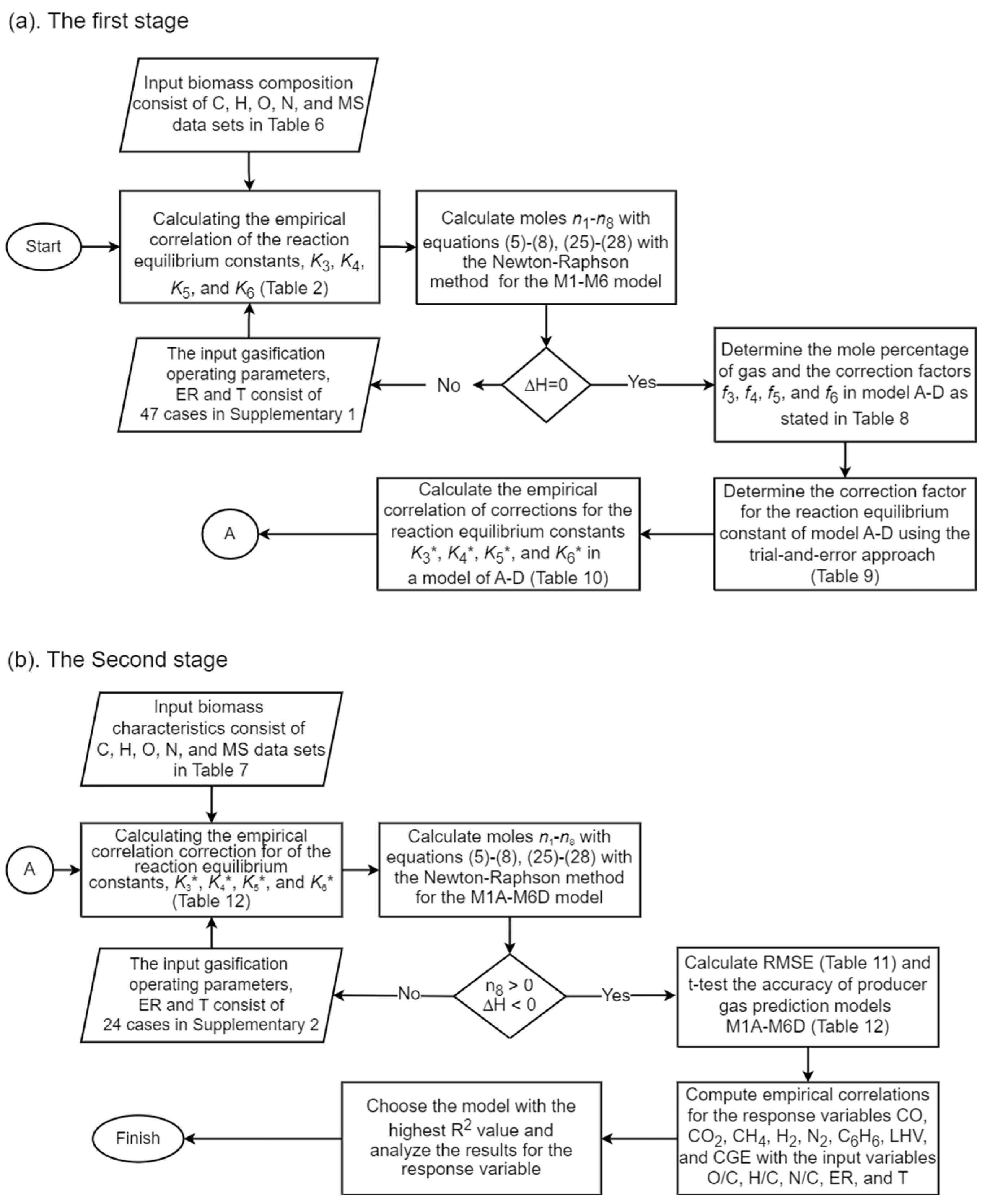
3.3. Algorithm of the Model Development

The algorithm to develop the stoichiometric models with correction factors and the new empirical correlation for the reaction equilibrium constants is shown in Figure 2. The first stage in developing the models was determining $n_1–n_8$, ln $K_i$, $f_k$, and finally, to obtain the empirical correlation of $K$*. Table 6 and Supplementary Table S1 were used as the inputs for this determination. The second stage was validating the models and testing their accuracy against the secondary data. Table 7 and Supplementary Table S2 were used as the inputs in the second stage.

4. Results and Discussion

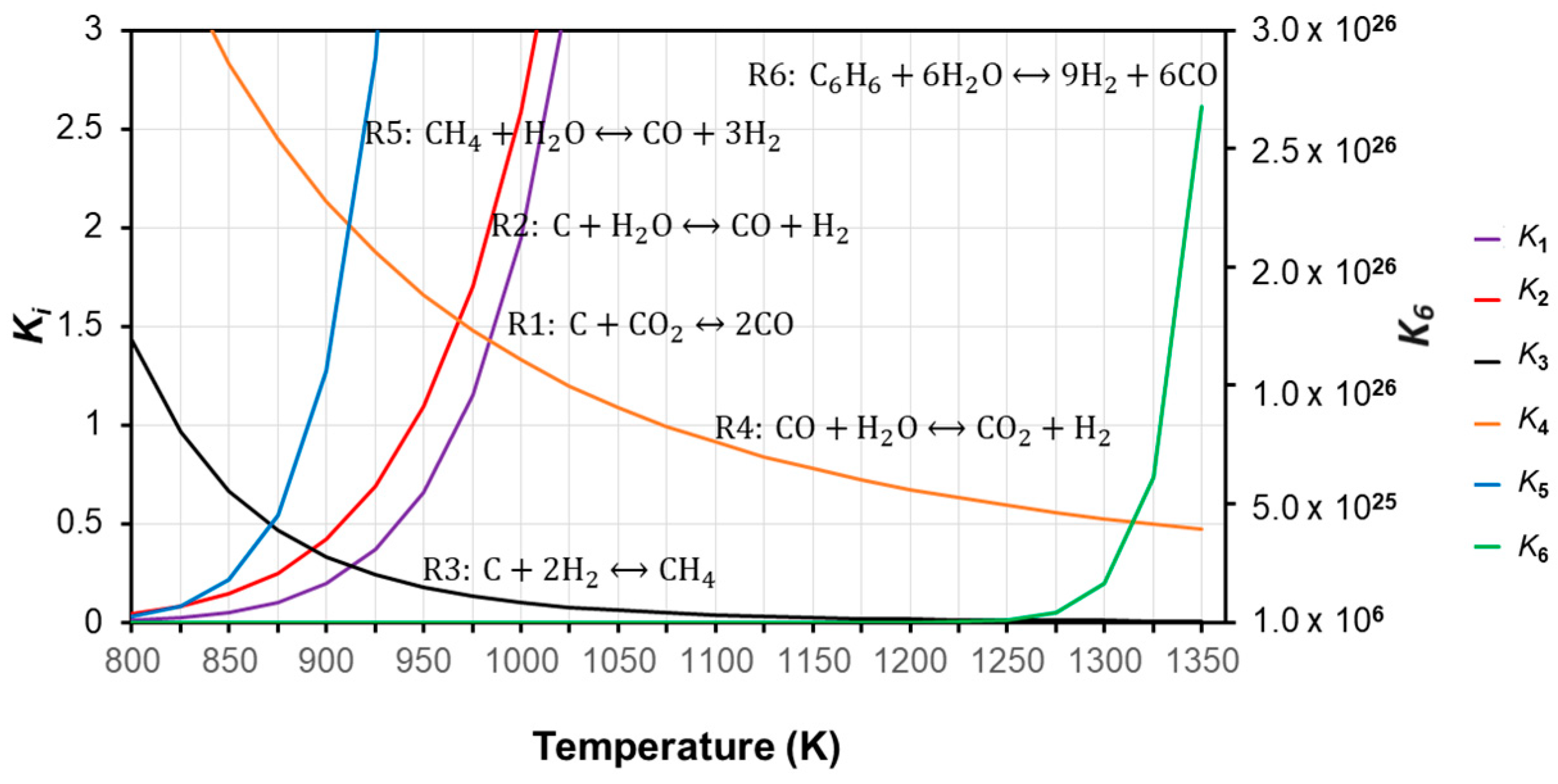
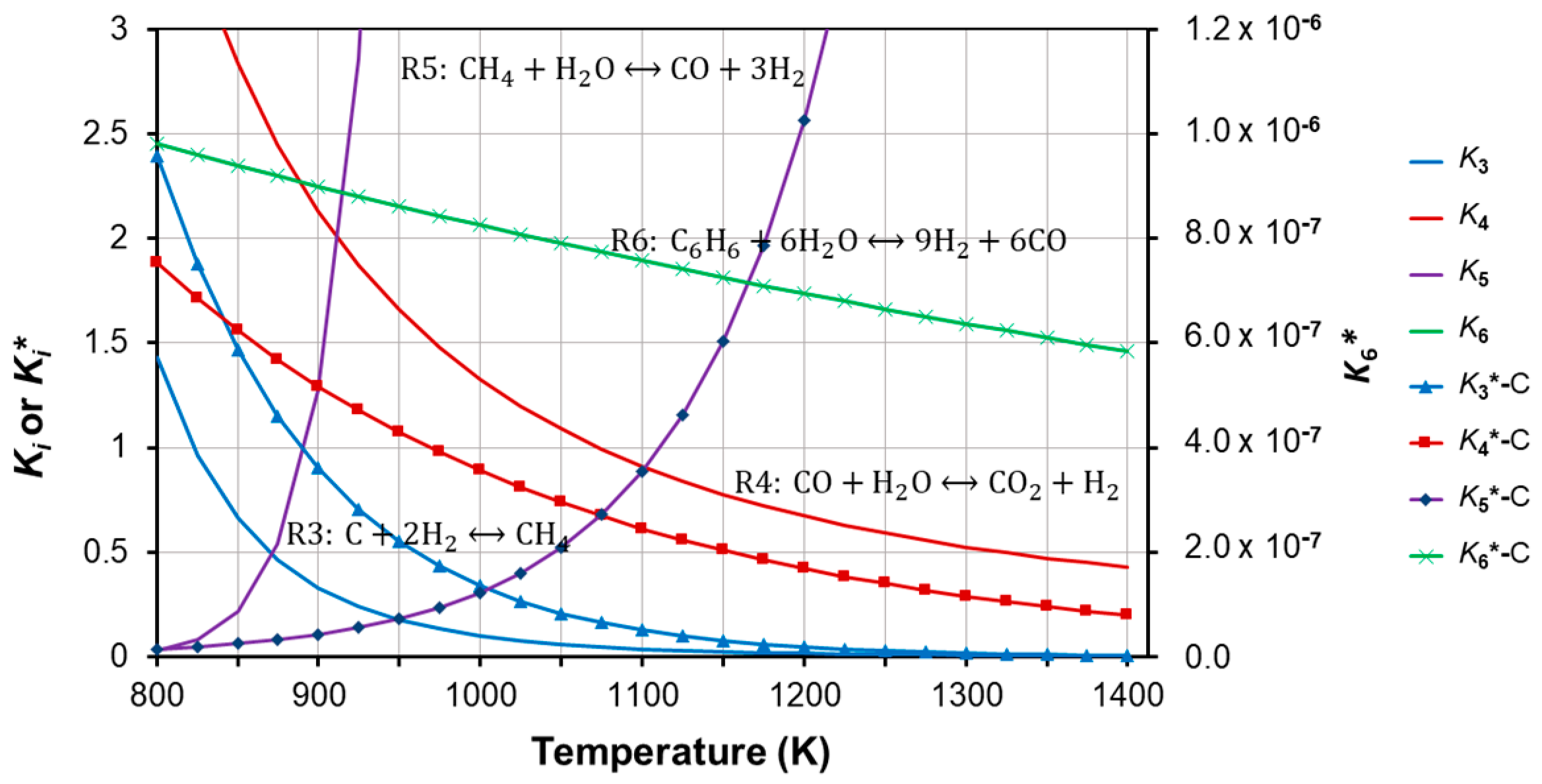
4.1. Correction Factors and New Empirical Correlation for the Equilibrium Constant

The correction factors based on the correlations in Table 5 were calculated, resulting in $f_3$, $f_4$, $f_5$, and $f_6$ for each model M1-M6. However, the correction factor $f_3$ obtained from M3 and M6 resulted in much different values than $f_3$ obtained from the other models. Therefore, the correction factors used for further study were those obtained from M1, M2, M4, M5. A combination of the correction factors ($f_3–f_6$) obtained from M1, M2, M4, and M5 were named as factor models A, B, C, and D, respectively.

Table 8. The correction factors obtained from M1, M2, M4, and M5.

Factor Model	Correction Factor
	${\mathit{f}}_3$	${\mathit{f}}_4$	${\mathit{f}}_5$	${\mathit{f}}_6$
A	14.7690	3.5143	0.0924	0.0092
B	66.4224	1.3221	0.0904	0.0513
C	33.9060	1.5202	0.0602	0.0054
D	305.3084	1.2181	0.0364	0.3595

displays the factor models under the condition of ΔH = 0.

The correction factors in each factor model were computed to Equation (42) to produce the new equilibrium constants $K$*. Combinations between M1–M6 and A–D (M1A–M6D) were applied during this computation step.

Table 9. The new reaction equilibrium constants (K*) for each factor model.

Factor Model	${\mathit{K}}_3^{\ast }$	${\mathit{K}}_4^{\ast }$	${\mathit{K}}_5^{\ast }$	${\mathit{K}}_6^{\ast }$
A	$2.2054K_3$	$0.7462K_4$	$0.1474{K_5}^{0.4325}$	$0.5568{K_6}^{0.0125}{T}^{-2}$
B	$3.2117K_3$	$0.5844K_4$	$0.1441{K_5}^{0.4325}$	$0.6898{K_6}^{0.0125}{T}^{-2}$
C	$2.7147K_3$	$0.6052K_4$	$0.0960{K_5}^{0.4325}$	$0.5203{K_6}^{0.0125}{T}^{-2}$
D	$4.7026K_3$	$0.5726K_4$	$0.0581{K_5}^{0.4325}$	$0.8800{K_6}^{0.0125}{T}^{-2}$

displays four new empirical correlations for the reaction equilibrium constant that corresponds to each factor model. These four correlations were found to have the lowest RMSE among 24 correlations developed from M1A–M6D.

Correction factors for the reaction equilibrium constant have been identified for some reactions. The correction factor for hydrogasification reaction (R3) is reported in the range of 0.2 [58] and 8.5216 [35], depending on the values of ER and/or T [20,59]. The correction factor for the water gas shift reaction (R4) ranges from 0.58 to 0.9677 [15], depending on the values of ER and/or T [14,59]. The correction factor for the methane decomposition reaction (R5) ranges from 0.0006 to 0.003 [60], and is dependent on the values of ER or T [14]. There is no correction factor reported for the steam reforming reaction (R6). Therefore, the empirical correlations of $K_i^{\ast }$ listed in Table 9, which also covers R6 were generalized as a temperature-dependent function as follows.

$$K_i^{\ast }=a_o\exp \left(a_{1}T\right)$$

(46)

The coefficient values of $a_o$ and $a_1$ in Equation (46) were determined by the linear regression method.

Table 10. Empirical correlation coefficient correction of reaction equilibrium constants.

Factor Models	Coefficient and R2-adj	${\mathit{K}}_3^{\ast }$	${\mathit{K}}_4^{\ast }$	${\mathit{K}}_5^{\ast }$	${\mathit{K}}_6^{\ast }$
A	a0	4289.2370	46.2788	1.1535 × 10−5	2.0959 × 10−6
	a1	−0.009770	−0.003742	0.010617	−0.000864
	R2-adj	0.9817	0.9725	0.9803	0.9998
B	a0	6246.2697	36.2444	1.1279 × 10−5	2.5967 × 10−6
	a1	−0.009770	−0.003742	0.010617	−0.000864
	R2-adj	0.9817	0.9725	0.9803	0.9998
C	a0	5939.6868	37.5318	7.5092 × 10−6	1.9585 × 10−6
	a1	−0.009770	−0.003742	0.010617	−0.000864
	R2-adj	0.9817	0.9725	0.9803	0.9998
D	a0	10,289.1435	35.5092	4.5442 × 10−6	3.3126 × 10−6
	a1	−0.00977	−0.00374	0.0106166	−0.000864
	R2-adj	0.9817	0.9725	0.9803	0.9998

presents the coefficients for calculating the new reaction equilibrium constant of hydrogasification processes (R3), water gas shift (R4), methane formation (R5), and steam reforming (R6), which are applicable within the temperature range of 800 to 1400 K.

In an equilibrium reaction, the constant of K = 1 means that the number of moles of reactant and product remains constant. If K < 1, the reaction is on the reactant side, implying that the number of reactants exceeds the number of products at equilibrium. Under conditions of K > 1, the reaction occurs on the product side, implying that the number of products exceeds the number of reactants at equilibrium. Figure 3 displays the relationship between $K_i$ and $K_i^{\ast }$ as function of temperature between 800 K and 1400 K, which was plotted using the empirical correlations presented in Table 2 and Table 10. The graph of $K_i^{\ast }$ plotted in Figure 3 was obtained by using factor model C. Figure 3 indicates an evident shift in the functions of $K_i$ and $K_i^{\ast }$. Consequently, the equilibrium temperatures of the following reactions also shift. The equilibrium temperature of R3 shifts from 850 K to 890 K, the temperature of R4 shifts from 1070 K to 960 K, the temperature of R5 shifts from 880 K to 1110 K, and R6 is shown to never reach equilibrium. The change of the equilibrium constant of the relevant reaction was further determined by the number of gas molecules produced during the gasification.

4.2. Simulation, Validation, and Accuracy of the Composition of Producer Gas Using the Developed Stoichiometric Models

The chemical composition of n₁–n₈ can be determined by solving Equations (5)–(8) and (25)–(28). The equilibrium constant of each reaction (R3, R4, R5, and R6) is computed using Equation (46), and the results in terms of ΔH, yield of tar, and RMSE of factor model A–D for each developed model M1–M6 are displayed in

Table 11. The predicted C₆H₆ (mol%), ΔH, and RMSE of each developed model (M1A–M6D).

	Model	A	B	C	D	Original Model
ΔH (kJ/kmol)	M1	−17,658	−9759	−17,603	−15,742	66,247
	M2	−16,135	−13,498	−14,367	−13,001	10,270
	M3	−16,144	−13,483	−14,389	−13,175	8787
	M4	−18,142	−14,542	−20,843	−18,112	69,783
	M5	−20,304	−17,526	−18,397	−17,199	1013
	M6	−20,564	−17,711	−20,050	−17,642	1680
C6H6 (%mol)	M1	1.691	1.245	1.746	1.700	−1.743
	M2	1.652	1.542	1.599	1.450	0.000
	M3	2.835	1.556	1.578	1.412	0.029
	M4	1.073	1.550	1.093	0.984	−2.268
	M5	1.094	0.998	1.045	0.908	0.024
	M6	1.099	1.018	1.028	0.885	0.000
RMSE (%)	M1	2.906	3.374	2.752	2.867	14.270
	M2	2.834	2.684	2.675	2.667	6.989
	M3	2.838	2.684	2.659	2.657	6.940
	M4	3.094	2.351	2.862	2.803	14.647
	M5	2.965	2.740	2.755	2.694	7.095
	M6	2.947	2.764	2.747	2.697	6.713

. The data in Table 7 were used as the model inputs. The data in Supplementary Table S2 were used to validate the predicted results by M1A–M6D.

Based on Table 11, the original stoichiometric models (M1O, M2O, M3O, M4O, M5O, and M6O) have average ΔH > 0, yield of C₆H₆ < 0, and RMSE > 10% (Table 11). These three indications are the challenges for using the original model to simulate the gas composition of biomass gasification. The results of ΔH, a yield of C₆H₆, and RMSE were improved when the factor model was introduced into the developed models (M1A-M6D). The average ΔH became less than 0, a yield of C₆H₆ was more than 0, and RMSE was smaller than 3.00%. Based on these three, the developed stoichiometric models with factor models are deemed to be valid. RMSE of the stoichiometric models developed in this study (M1A–M6D) are in line with the RMSE of the stoichiometric models developed by Ayub et al. [15]. The models had RMSE values between 2.3018 and 2.7718. The stoichiometric models developed by Aydin et al. [20] that were tested against 32 experimental cases had RSME ranges from 3.854 to 3.3373, which were more than 3%. Semi-empirical modified models by Silva et al. [5] resulted in RMSE between 2.39 and 4.25 over 64 simulation scenarios. Mendiburu et al. [34] found similar values of RMSE by modifying the stoichiometric models.

Table 12. The predicted values of producer gas and their statistical analysis.

Model	CO (%vol)	CO2 (%vol)	CH4 (%vol)	H2 (%vol)	N2 (%vol)	t-Stat CO	t-Stat CO2	t-Stat CH4	t-Stat H2	t-Stat N2
M1O	36.190	2.159	0.395	28.362	34.637
M1A	17.399	13.998	0.261	14.985	51.666	−0.943	2.960	−8.836	2.829	−1.827
M1B	20.736	11.913	0.458	16.110	49.539	4.787	−0.373	−7.995	5.045	−4.460
M1C	18.065	13.486	0.313	14.031	52.358	0.214	2.145	−8.631	0.882	−0.956
M1D	18.582	13.332	0.528	13.903	51.956	1.043	1.816	−7.694	0.525	−1.408
M2O	25.002	9.124	0.307	21.165	44.403
M2A	17.489	13.926	0.311	14.920	51.702	−0.877	2.857	−8.707	2.756	−1.742
M2B	19.121	12.804	0.389	14.505	51.639	2.329	1.051	−8.431	1.954	−1.834
M2C	18.710	13.071	0.360	14.424	51.835	1.519	1.478	−8.516	1.765	−1.590
M2D	19.448	12.633	0.611	14.418	51.440	3.015	0.774	−7.183	1.817	−2.078
M3O	24.924	9.133	0.363	21.511	44.040
M3A	17.764	14.190	0.321	15.164	52.562	−0.359	3.252	−8.725	3.231	−0.683
M3B	19.120	12.785	0.323	14.543	51.673	2.348	1.022	−8.760	2.037	−1.811
M3C	18.727	13.077	0.443	14.357	51.819	1.560	1.494	−8.111	1.635	−1.605
M3D	19.461	12.656	0.761	14.302	51.408	3.049	0.807	−6.087	1.563	−2.105
M4O	36.402	1.747	0.386	29.540	34.193
M4A	17.144	13.802	0.320	16.189	51.471	−1.374	2.610	−8.678	5.173	−1.983
M4B	20.152	12.021	0.582	17.405	49.162	4.071	−0.191	−7.144	7.348	−4.523
M4C	17.598	13.364	0.386	15.061	52.498	−0.541	1.840	−8.259	3.137	−0.771
M4D	18.344	12.949	0.634	15.036	52.054	0.635	1.220	−6.885	3.139	−1.328
M5O	24.520	9.061	0.273	21.994	44.128
M5A	16.741	13.951	0.344	15.496	52.374	−2.267	2.905	−8.589	3.832	−0.889
M5B	18.366	12.829	0.416	15.021	52.371	0.803	1.091	−8.229	2.962	−0.898
M5C	17.966	13.089	0.393	14.971	52.537	0.045	1.512	−8.342	2.835	−0.694
M5D	18.645	12.697	0.659	14.898	52.193	1.336	0.871	−6.761	2.836	−1.110
M6O	23.943	9.367	0.160	21.743	44.763
M6A	16.744	13.944	0.320	15.517	52.375	−1.473	2.658	−8.919	3.770	−1.147
M6B	18.370	12.807	0.322	15.101	52.382	1.630	0.837	−8.910	2.975	−1.155
M6C	18.130	13.287	0.436	14.952	52.167	0.295	1.979	−8.405	3.055	−1.197
M6D	18.653	12.711	0.754	14.823	52.174	2.216	0.678	−6.041	2.615	−1.402

presents the mean of the predicted composition of CO, CO₂, CH₄, H₂, and N₂ gas simulated using M1A–M6D. The models of M1D, M2C, and M3C accurately predicted composition of CO, CO₂, H₂, and N₂ (α = 0.05 and t-crit value of 2.0687). M1B accurately predicted CO, H₂, and N₂. M2D and M3B accurately estimated CO₂, H₂, and N₂. The models M4C, M4D, M5C, M5D, M5B, M6C, and M6D correctly predicted CO, CO₂, and N₂. The predicted composition of CH₄ by all developed models (M1A–M6D) was lower than the experimental data. Based on the statistical analysis, the developed models M1D, M2C, and M3C are the models that may accurately predict CO, CO₂, H₂, and N₂ gas composition.

4.3. Empirical Correlation between Independent and Dependent Variables in Biomass Gasification

Table 11 and Table 12 show predicted compositions of CO, CO₂, CH₄, H₂, N₂, and tar-(C₆H₆) by the models M1A–M6D. However, the models cannot be used to establish sensitivity correlations between independent and dependent variables in biomass gasification. Therefore, an empirical correlation derived from the models needs to be established to evaluate how changes in input variables affect compositions of CO, CO₂, CH₄, H₂, N₂, and tar-(C₆H₆) gas. Subramanian et al. [45] developed a second-order polynomial equation to correlate volatile matter (VM) and fixed carbon (FC) with the composition of CO, H₂, and CH₄. Pio et al. [61] established multiple linear correlations with ER and temperature (T) as independent variables to estimate the composition of CO, CH₄, and H₂ gas. Buragohian et al. [62] established a correlation between T, air flow ratio (AR), hydrogen-to-carbon (H/C), and oxygen-to-carbon (O/C) ratio with LHV, yield, and composition of syngas. Chen et al. [63] applied the response surface method to develop a second-order polynomial correlation between ER, T, and time as the independent variables with the composition of syngas, whereas Rupesh et al. [58] used multiple linear regression to predict CO, CO₂, H₂, and N₂ gas. The results of this study indicated that models M1D, M2C, and M3C have good validity and accuracy in simulating producer gas composition from biomass gasification. Further, one of these models was used to establish an empirical correlation between O/C, H/C, N/C, ER, and T as the independent variables and CO, CO₂, CH₄, H₂, N₂, C₆H₆ content, LHV-gas, and CGE as the dependent variables. The M2C model was selected for this establishment because the multivariable regression coefficient of determination for each response variable is the largest compared with the M1D and M3C models. Based on M2C model, the following empirical correlation between the independent and dependent variables in biomass gasification is set up.

$$X=a_0{\left(\frac{H}{C}\right)}^{a_1}{\left(\frac{O}{C}\right)}^{a_2}{\left(\frac{N}{C}\right)}^{a_3}{\left(ER\right)}^{a_4}{T}^{a_5}$$

(47)

Unlike the correlation established by Buragohian et al. [62], the correlation in Equation (47) uses ER instead of AR and includes the ratio of H/C, O/C, and N/C. The X variable is the dependent variable that includes CO, CO₂, CH₄, H₂, N₂ in % mol, C₆H₆ (g/Nm³), LHV-gas (MJ/Nm³), and CGE (%). Further, Equations (48)–(52) were established based on Equation (47) and the predicted data by the M2C model. The empirical correlations described by Equations (48)–(53) were further used to investigate the impact of independent variables on the dependent variables.

$$\mathrm{C}\mathrm{O}=0.0020{\left(\frac{H}{C}\right)}^{-0.2908}{\left(\frac{O}{C}\right)}^{0.1062}{\left(\frac{N}{C}\right)}^{-0.0108}{ER}^{-0.1760}{T}^{1.2869};R^2\mathrm{a}\mathrm{d}\mathrm{j}=0.9815$$

(48)

$$\mathrm{C}{\mathrm{O}}_2=1.1650\times {10}^6{\left(\frac{H}{C}\right)}^{-0.4372}{\left(\frac{O}{C}\right)}^{0.7438}{\left(\frac{N}{C}\right)}^{0.0005}{ER}^{-0.1184}{T}^{-1.5803};R^2\mathrm{a}\mathrm{d}\mathrm{j}=0.9931$$

(49)

$$\mathrm{C}{\mathrm{H}}_4=2.0071\times {10}^{40}{\left(\frac{H}{C}\right)}^{1.4861}{\left(\frac{O}{C}\right)}^{0.7418}{\left(\frac{N}{C}\right)}^{-0.0315}{ER}^{-0.2936}{T}^{-13.5810};R^2\mathrm{a}\mathrm{d}\mathrm{j}=0.9960$$

(50)

$${\mathrm{H}}_2=7719.5233{\left(\frac{H}{C}\right)}^{0.7330}{\left(\frac{O}{C}\right)}^{0.4827}{\left(\frac{N}{C}\right)}^{-0.0139}{ER}^{-0.2531}{T}^{-0.9627};R^2\mathrm{a}\mathrm{d}\mathrm{j}=0.9354$$

(51)

$${\mathrm{C}}_6{\mathrm{H}}_6=6.1558\times {10}^{12}{\left(\frac{H}{C}\right)}^{0.9082}{\left(\frac{O}{C}\right)}^{-3.2235}{\left(\frac{N}{C}\right)}^{-0.1833}{ER}^{-1.4669}{T}^{-4.2424};R^2\mathrm{a}\mathrm{d}\mathrm{j}=0.8634$$

(52)

$${\mathrm{L}\mathrm{H}\mathrm{V}}_{\mathrm{g}\mathrm{a}\mathrm{s}}=0.4931{\left(\frac{H}{C}\right)}^{0.0328}{\left(\frac{O}{C}\right)}^{0.0370}{\left(\frac{N}{C}\right)}^{-0.0162}{ER}^{-0.6884}{T}^{0.2085};R^2\mathrm{a}\mathrm{d}\mathrm{j}=0.9950$$

(53)

$$CGE=29.8215{\left(\frac{H}{C}\right)}^{0.1308}{\left(\frac{O}{C}\right)}^{0.3723}{\left(\frac{N}{C}\right)}^{-0.0128}{ER}^{0.0115}{T}^{0.1178};R^2\mathrm{a}\mathrm{d}\mathrm{j}=0.8423$$

(54)

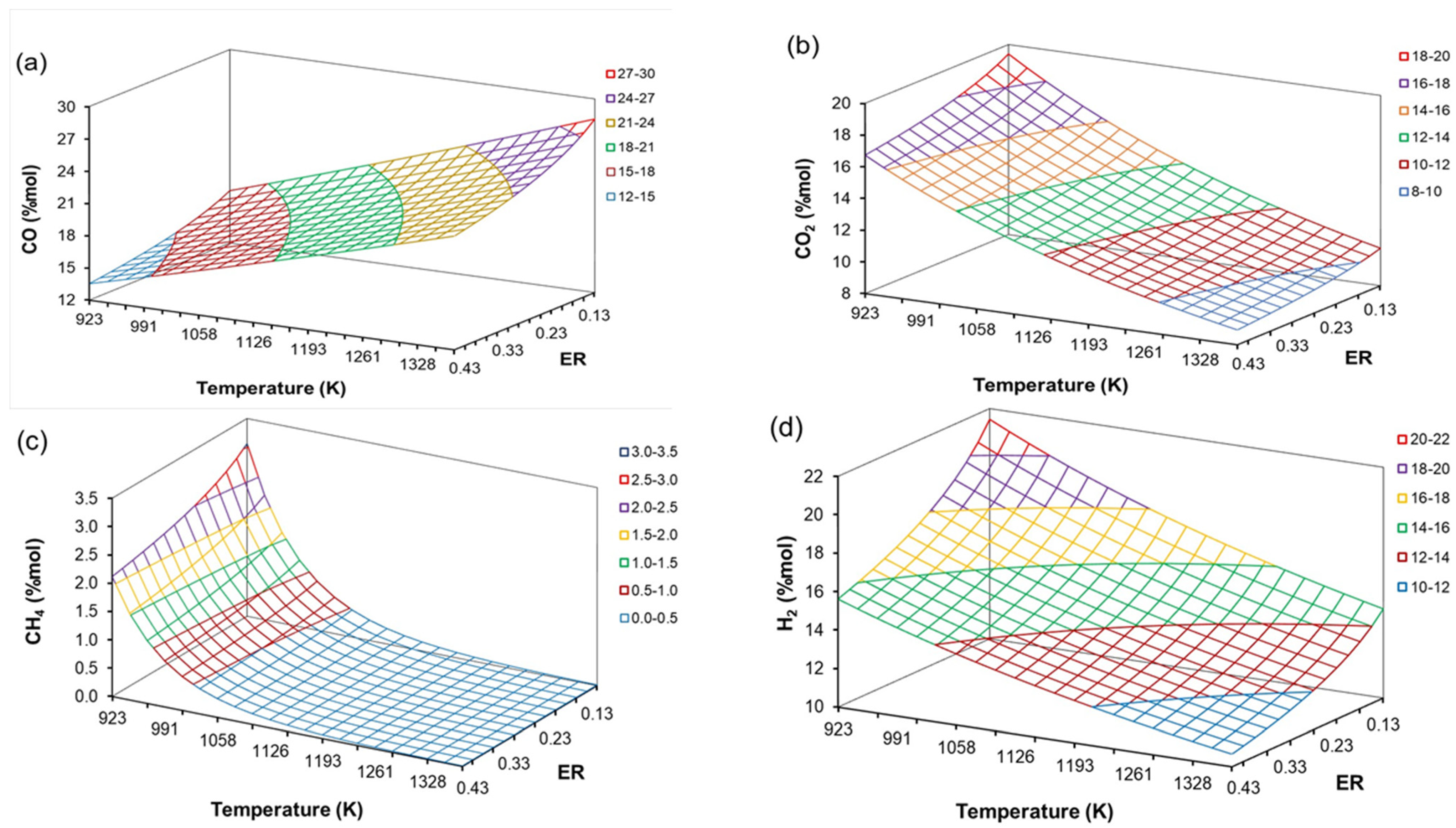
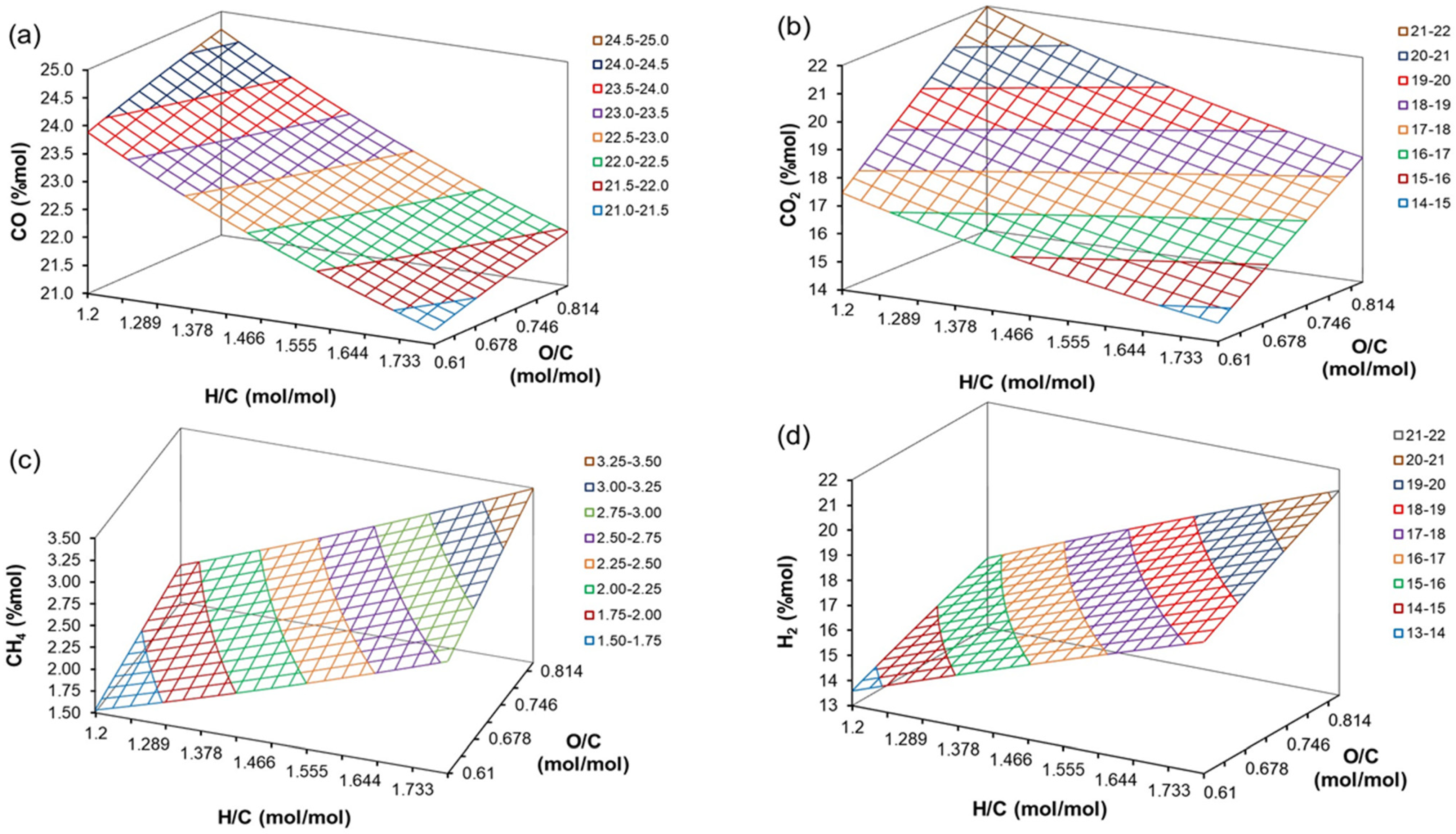
4.4. The Effect of H/C, O/C, ER, and T on Producer Gas Composition

The results obtained from Equations (48)–(51) have determination coefficients (R²-adj) that are larger than 0.9354. Based on the sensitivity analysis, the results indicated that temperature has the biggest influence on the composition of producer gas. Figure 4 shows that, under constant O/C, H/C, and N/C, the highest CO that was simulated occurred at low ER and high T, whereas the highest CO₂, CH₄, and H₂ were predicted to occur at both low ER and T. The results could be attributed to the reaction equilibrium constants $K_i^{\ast }$ during reactions within gasification, which has been displayed in Figure 3. Figure 3 shows that R3 has K₃* < 1 at T > 890 K. This indicates that the reaction would result in a higher proportion of H₂ than CH₄. In the case of R4 occurs at T > 970 K, K₄ shifts into K₄* and K₄* < 1. As a result, R4 would result in more CO than CO₂ and H₂. The same holds for the shifting from K₅ to K₅* at temperatures greater than 1110 K. K₅* > 1, which triggers R5 when to produce more CO and H₂ than CH₄. R6 would produce more C₆H₆ than H₂ and CO because K₆* is always less than 1 when shifting from K₆ to K₆* occurs. Low temperatures (900–1273 K) gasification [64,65] would trigger R3 to produce more H₂, whereas R4 produces more CO, CO₂, and H₂. The reaction R5 and R6 would be responsible for producing CH₄ and C₆H₆. High gasification temperatures (T > 1273 K) would lead to the production of H₂ by R3, CO by R4, CO, and H₂ by R5 and C₆H₆ by R6.

Other studies [10,18,19,65,66] show that the percentage of CO increases while the percentages of CO₂, CH₄, and H₂ decrease with increasing temperature. In contrast, some studies also show that the percentage of CO and H₂ decreases [42,45,67,68] with increasing temperature. It seems that increasing gasification temperature may result in different compositions of producer gas. The composition of producer gas does not only depend on the temperature, but it also depends on the ER. Figure 4 shows that the compositions of CO, CO₂, CH₄, and H₂ decrease with increasing ER. The ER changes significantly affect the composition of CO and H₂, which may be explained by the oxidation zone. In the oxidation zone, series of isothermal processes (C + O₂ = CO₂), (C + ½O₂ = CO), (H₂ + ½O₂ = H₂O), and (CO + ½O₂ = CO₂) produce heat [3]. As ER rises, the airflow in the reactor increases. Increasing air in the oxidation zone would affect the reactions of carbon, carbon dioxide, and hydrogen with oxygen. These reactions yield CO₂ and H₂O [10,65]. The reaction between CO₂ and H₂O would subsequently be employed in the reduction zone. If the airflow in the reactor is too low, C will not be burned into CO, CO₂, and CH₄. Therefore, increasing ER leads to the reduction of CO, CO₂, H₂, and CH₄ [18,65,69,70].

Equations (48)–(51) were further applied to simulate the effects of O/C and H/C on the composition of producer gas, under constant N/C, ER, and T. At N/C of 0.0198, ER of 0.332, and T of 1128 K, the lowest predicted composition of CO and CO₂ were 21.253% and 14.651% mol, respectively. These values were obtained at O/C of 0.71 and H/C of 1.792. The lowest predicted composition of CH₄ and H₂ were 1.531% and 13.584% mol, respectively, which occurred at O/C and H/C of 0.61 and 1.2, respectively. The highest predicted composition of CH₄ and H₂, i.e., 1.531% and 13.584% mol, respectively, were obtained with O/C and H/C of 0.831 and H/C of 1.792, respectively. Based on the simulation above, the biomass gasification process should be carried out under high O/C but low H/C to obtain the maximum CO and CO₂. Both O/C and H/C should be high to obtain the maximum CH₄ and H₂.

This is in line with the simulation shown in Figure 5, which demonstrates increasing CH₄ and H₂ with H/C. In contrast, the CO and CO₂ decrease. Increasing CO, CO₂, CH₄, and H₂ is simulated with increasing O/C. H₂ and CH₄ are produced from endothermic reactions, and the production may continue with an increase in the H/C ratio during the gasification process. Therefore, biomass that is rich in hydrogen content may produce more H2 or CH4. Pradhan et al. [27] found that the hydrogen content of a biomass lowers CO and CO₂, but increases H₂ and CH₄. Exothermic reaction may occur when the biomass is rich in oxygen content. Increasing the O/C ratio would increase the compositions of CO, CH₄, and H₂. Similar findings are reported in other studies [27,48,62].

Aside from the processing parameters inside a reactor, the compositions of producer gas are also affected by the properties of biomasses. Biomass usually consists of cellulose (30–60%), hemicellulose (15–25%), and lignin (20–40%). On the Van Krevelen diagram (Figure 6), lignin has the lowest H/C and O/C ratio, whereas cellulose has the highest ratios [64]. Biomasses rich in hemicellulose and lignin are usually selected for gasification [71,72]. The C-H-O ternary diagram indicates that a biomass with a high H/C ratio produces more CH₄ and H₂, whereas a biomass with a high O/C ratio produces more CO and CO₂ [71].

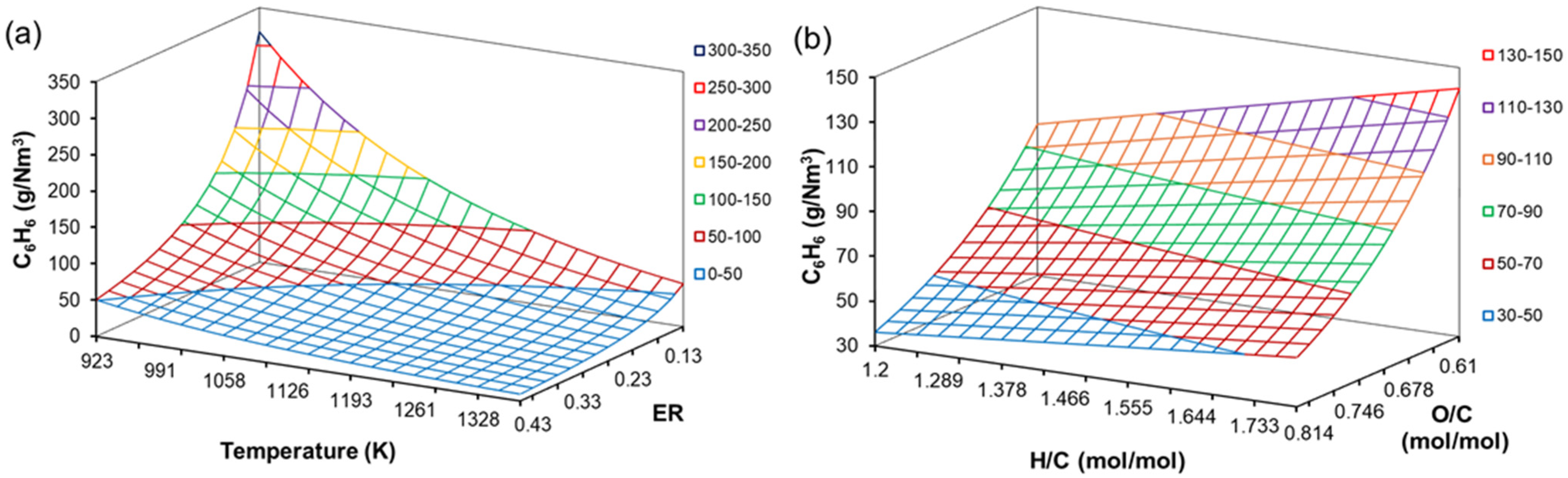
4.5. Effect of H/C, O/C, ER and T on Tar Content

Tar produced by gasification is also affected by the biomass type, temperature, ER, and reactor [17]. The existence of tar in the producer gas is problematic when syngas is used for internal combustion engines [20]. The maximum tar concentration in producer gas that is allowed for internal combustion engines is 100 mg/Nm³ [19]. The models M1A-M6D predicted the composition of tar in the form of C₆H₆ in the range of 0. 885 and 2.835 mol% (Table 11). If this percentage is converted to gr/Nm³, Equation (45) yields 23,584–98,733 g/Nm³ tar in the producer gas. The simulation shows that the producer gas satisfies the maximum tar requirement if it is applied as internal engine fuel. Equation (52) describes that the tar concentration (g/Nm³) is sensitive to changes in temperature and O/C ratio. Figure 7 depicts the response of tar concentration to the changes of (a) ER and T, (b) H/C and O/C.

Figure 7 shows that biomass with a high H/C and O/C ratio produces a high concentration of tar when T and ER are low. The tar concentration decreases with increasing T and ER. Tar content falls when H/C lowers and O/C increases. Figure 7a may be obtained if the ER is low and the temperature is high. Figure 7a can still be obtained at low a temperature, but the ER must be high. The results suggest that minimum tar production during biomass gasification could be obtained at T > 1073 K. The steam reforming process, as described in Equation (14), may reduce tar production at high-temperature ER. Conversely, the original models cannot predict tar content in the producer gas. The reaction constant in the original model $K_6$was more than 1. By modifying the models, $K_6^{\ast }$ < 1, and the models accurately predicted the tar concentration.

The results of the tar concentration simulated in this study are in line with the experimental findings of other studies. Gasification of corn straw with a downdraft reactor at an ER of 0.18 to 0.41 produced tar at concentrations of 7215 to 4617 mg/Nm³ [73]. Gasification of the same biomass with a downdraft reactor at an ER of 0.2 to 0.28 produced tar with concentrations in the range of 369 and 67 g/Nm³ [38]. Gasification of corn cob at ER of between 0.2 and 0.4 yielded tar with concentration from 1.7 to 2.4 mg/Nm³; whereas the wood waste gasifier in the same setup resulted in 1.85 to 3.1 g/Nm³ tar [74]. Gasification of MSW at an ER of 0.3 to 0.5 yielded a decreasing tar from 328.69 to 31.45 mg/Nm³, respectively [40]. The tar concentration in the producer gas decreased from 418.95 to 78.57 g/Nm³ when the temperature of eucalyptus gasification was increased from 663.71 to 793.56 °C [56]. Another study also shows that tar concentration fell from 9.4 to 7.1 g/Nm³ after the temperature was increased from 700 to 850 °C, respectively [75].

4.6. Effect of H/C, O/C, ER, and T on LHV-Gas

The heating value of syngas for internal combustion engines must be between the range of 5.02 to 7.47 MJ/Nm³ [76] Hence, the calorific value has significant importance in the biomass gasification process. This value is determined by the gas composition of CO, CH₄, H₂, and C₆H₆. Equation (53) indicates that changes in the ${\mathrm{L}\mathrm{H}\mathrm{V}}_{\mathrm{g}\mathrm{a}\mathrm{s}}$ (MJ/Nm³) are significantly affected by variations of ER and temperature. Figure 8 depicts the response of ${\mathrm{L}\mathrm{H}\mathrm{V}}_{\mathrm{g}\mathrm{a}\mathrm{s}}$ as a function of (a) ER and T, as well as (b) H/C and O/C ratios.

Figure 8a illustrates that the highest LHV_gas could be obtained at low ER and high T, under constant O/C, H/C, and N/C. The highest LHV_gas could also be obtained at high O/C and H/C ratios under constant N/C, ER, and T (Figure 8b). Therefore, selecting biomass with high H/C and O/C ratios is important to get high ${\mathrm{L}\mathrm{H}\mathrm{V}}_{\mathrm{g}\mathrm{a}\mathrm{s}}$ during gasification by maintaining low ER and high T during the process. Biomass with a high H/C ratio also leads to more production of H₂ and CH₄, whereas a high O/C ratio promotes more production of CO and CO₂. The simulation depicted in Figure 8 is in line with other experimental studies. Gasification of palm kernel oil biomass at 850–950 °C. increases LHV from 4.02 to 4.65 MJ/Nm³, compared to the literature. ${\mathrm{L}\mathrm{H}\mathrm{V}}_{\mathrm{g}\mathrm{a}\mathrm{s}}$ rises from 4.49 to 5.15 MJ/Nm₃ at 720–802 °C [44]. In rice husk pellet gasification trials at 700–850 °C, ${\mathrm{L}\mathrm{H}\mathrm{V}}_{\mathrm{g}\mathrm{a}\mathrm{s}}$ rose from 4.19 to 5.86 MJ/Nm³ [56]. Gasification with ER 0.20 and ${\mathrm{L}\mathrm{H}\mathrm{V}}_{\mathrm{g}\mathrm{a}\mathrm{s}}$ 3.21 MJ/Nm³ [70]. The ER biomass MSW fluidized bed reactors between 0.2 and 0.4, ${\mathrm{L}\mathrm{H}\mathrm{V}}_{\mathrm{g}\mathrm{a}\mathrm{s}}$ reduced MJ/Nm³ from 12.40 to 11.23 [31]. RDF gasification at 0.2–0.6, ${\mathrm{L}\mathrm{H}\mathrm{V}}_{\mathrm{g}\mathrm{a}\mathrm{s}}$ lowers from 12.77 to 12.50 MJ/Nm³. ${\mathrm{L}\mathrm{H}\mathrm{V}}_{\mathrm{g}\mathrm{a}\mathrm{s}}$ declines around 0.14–0.3 ER. From 700 to 850 °C, ${\mathrm{L}\mathrm{H}\mathrm{V}}_{\mathrm{g}\mathrm{a}\mathrm{s}}$ climbs from 5.76 to 6.32 MJ/Nm³ [77] ${\mathrm{L}\mathrm{H}\mathrm{V}}_{\mathrm{g}\mathrm{a}\mathrm{s}}$ decreases as ER grows [78] Other empirical correlations corroborate that ${\mathrm{L}\mathrm{H}\mathrm{V}}_{\mathrm{g}\mathrm{a}\mathrm{s}}$ rises as temperature rises, ER drops, H/C and O/C rise, and ${\mathrm{L}\mathrm{H}\mathrm{V}}_{\mathrm{g}\mathrm{a}\mathrm{s}}$ rise. [61,62]. Many empirical correlations and experimental studies reveal that when temperatures rise, ER drops, H/C and O/C ratios rise, and the heating value rises.

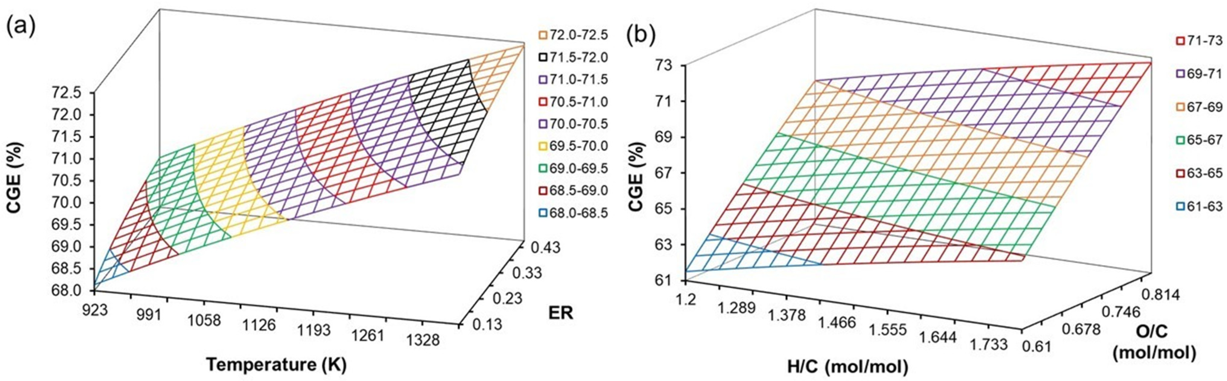
4.7. Effect of H/C, O/C, ER, and T on CGE

Cold gasification efficiency (CGE) is a measurement of gasification performance [79] Several factors affect CGE, including biomass type, reactor type, particle size, temperature, and reactor type [80] Equation (54) was developed to evaluate the effect of N/C, O/C, H/C, ER, and T on CGE. Equation (54) indicates that the concentrations of oxygen, hydrogen, and carbon have a significant impact on biomass CGE. Figure 9 shows the different O/C and H/C ratios on CGE (%).

Figure 9a illustrates that CGE increases with ER and T under constant H/C, O/C, and N/C. Likewise, the CGE would increase with increasing H/C and O/C of the biomass under constant gasification operational parameters as can be seen in Figure 9b. The positive correlation of CGE with ER and T is in line with experimental studies. The CGE of woodchip gasification increased from 45.6% to 61.9% when the gasification temperature was increased from 558 to 612 °C, respectively [79]. Rice husk gasification at a constant ER of 0.3 yielded CGE of 39.1% at a gasification temperature of 800 °C. The CGE value increased to 69.5% when the gasification temperature was raised to 1400 K. Similar trend was also shown with biomasses from sugarcane and palm kernel [81] The positive correlation of CGE with gasification temperature has also been shown by other empirical findings [82,83]. Positive correlation of CGE with ER has also been proven experimentally. Park et al. [31] used downdraft fixed bed (DFB) and bubbling fluidized bed (BFB) reactors to gasify solid refuse fuel (SRF) with ER values between 0.2 and 0.6. The CGE of the gasification increased from 47.76% to 51.44% in DFB reactor and from 61.4% to 67.25% in BFB reactor. Another study showed that a small increment of ER significantly increases CGE. Increasing ER values from 0.23 to 0.26 increased CGE from 58% to 65% [64]. Arun et al. [57] found that CGE reached its highest values at ER of 0.35, i.e., 72.74%—CC-78.37%, and decreased when the ER was beyond 0.35. However, another study found that the CGE reached 79.46% at ER of 0.378 when lignin-rich biomass was gasified.

5. Conclusions

This study developed stoichiometric models that involve correction factors for the reaction equilibrium constant. The developed models focus on reducing errors, predicting tar content, and applying steam reforming reactions. Six stoichiometric models (M1–M6) with four-factor models (A–D) and equilibrium constants ($K_3^{\ast }–K_6^{\ast }$) were developed in this study, resulting in 24 model combinations with the following details.

• All models can predict the composition of the producer gas with an RMSE of less than 3.5%.
• All models can predict the concentration of tar (C₆H₆) in gas producers through using steam reforming reactions in the modeling process.
• Only three models (M1D, M2C, and M3C) out of 24 models showed high accuracy in predicting CO, CO₂, H₂, and N₂ gas concentration.
• Model M2C can be further used to develop empirical correlations that include H/C, O/C, and N/C.
• The empirical correlation models have power function equations that include biomass content and gasification operating parameters (H/C, O/C, N/C, ER, and T) as the input variables.
• The empirical correlations estimated the composition of CO, CO₂, CH₄, H₂, and tar content (C₆H₆), LHV, and CGE with R² of prediction of each composition was 0.9815, 0.9931, 0.9960, 0.9354, 0.8634, 0.9950, and 0.8423, respectively. These results confirmed that the inclusion of H/C, O/C, and N/C into the models makes the models more reliable.

The empirical correlations developed in this study will be beneficial for identifying the most appropriate biomass to be a gasifier, designing gasification operating parameters, and predicting the resulting producer gas and tar composition, LHV, and CGE values.

References

1. Situmorang, Y.A.; Zhao, Z.; Yoshida, A.; Abudula, A.; Guan, G. Small-Scale Biomass Gasification Systems for Power Generation (<200 kW Class): A Review. Renew. Sustain. Energy Rev. 2020, 117, 109486. [Google Scholar] [CrossRef]
2. Suparmin, P.; Nurhasanah, R.; Hendri, H.; Ridwan, M. Biomass for Dual-Fuel Syngas Diesel Power Plants. Part I: The Effect of Preheating on Characteristics of the Syngas Gasification of Municipal Solid Waste and Wood Pellets. Arab. J. Basic. Appl. Sci. 2023, 30, 378–392. [Google Scholar] [CrossRef]
3. Silva, I.P.; Lima, R.M.A.; Silva, G.F.; Ruzene, D.S.; Silva, D.P. Thermodynamic Equilibrium Model Based on Stoichiometric Method for Biomass Gasification: A Review of Model Modifications. Renew. Sustain. Energy Rev. 2019, 114, 109305. [Google Scholar] [CrossRef]
4. Sudarmanta, B.; Sampurno; Dwiyantoro, B.A.; Gemilang, S.E.; Putra, A.B.K. Performance Characterization of Waste to Electric Prototype Uses a Dual Fuel Diesel Engine and a Multi-Stage Downdraft Gasification Reactor. Mater. Sci. Forum 2019, 964, 80–87. [Google Scholar] [CrossRef]
5. Silva, I.P.; Lima, R.M.A.; Santana, H.E.P.; Silva, G.F.; Ruzene, D.S.; Silva, D.P. Development of a Semi-Empirical Model for Woody Biomass Gasification Based on Stoichiometric Thermodynamic Equilibrium Model. Energy 2022, 241, 122894. [Google Scholar] [CrossRef]
6. Loha, C.; Gu, S.; De Wilde, J.; Mahanta, P.; Chatterjee, P.K. Advances in Mathematical Modelling of Fluidized Bed Gasification. Renew. Sustain. Energy Rev. 2014, 40, 688–715. [Google Scholar] [CrossRef]
7. Safarian, S.; Unnþórsson, R.; Richter, C. A Review of Biomass Gasification Modelling. Renew. Sustain. Energy Rev. 2019, 110, 378–391. [Google Scholar] [CrossRef]
8. Molino, A.; Larocca, V.; Chianese, S.; Musmarra, D. Biofuels Production by Biomass Gasification: A Review. Energies 2018, 11, 811. [Google Scholar] [CrossRef]
9. Safarian, S.; Unnthorsson, R.; Richter, C. The Equivalence of Stoichiometric and Non-Stoichiometric Methods for Modeling Gasification and Other Reaction Equilibria. Renew. Sustain. Energy Rev. 2020, 131, 109982. [Google Scholar] [CrossRef]
10. Watson, J.; Zhang, Y.; Si, B.; Chen, W.T.; de Souza, R. Gasification of Biowaste: A Critical Review and Outlooks. Renew. Sustain. Energy Rev. 2018, 83, 1–17. [Google Scholar] [CrossRef]
11. Ibrahim, A.; Veremieiev, S.; Gaskell, P.H. An Advanced, Comprehensive Thermochemical Equilibrium Model of a Downdraft Biomass Gasifier. Renew. Energy 2022, 194, 912–925. [Google Scholar] [CrossRef]
12. Kaydouh, M.N.; El Hassan, N. Thermodynamic Simulation of the Co-Gasification of Biomass and Plastic Waste for Hydrogen-Rich Syngas Production. Results Eng. 2022, 16, 100771. [Google Scholar] [CrossRef]
13. Samadi, S.H.; Ghobadian, B.; Nosrati, M. Prediction and Estimation of Biomass Energy from Agricultural Residues Using Air Gasification Technology in Iran. Renew. Energy 2020, 149, 1077–1091. [Google Scholar] [CrossRef]
14. Said, M.S.M.; Ghani, W.A.W.A.K.; Tan, H.B.; Ng, D.K.S. Prediction and Optimisation of Syngas Production from Air Gasification of Napier Grass via Stoichiometric Equilibrium Model. Energy Convers. Manag. X 2021, 10, 100057. [Google Scholar] [CrossRef]
15. Ayub, H.M.U.; Park, S.J.; Binns, M. Biomass to Syngas: Modified Stoichiometric Thermodynamic Models for Downdraft Biomass Gasification. Energies 2020, 13, 5383. [Google Scholar] [CrossRef]
16. Kushwah, A.; Reina, T.R.; Short, M. Modelling Approaches for Biomass Gasifiers: A Comprehensive Overview. Sci. Total Environ. 2022, 834, 155243. [Google Scholar] [CrossRef] [PubMed]
17. Valderrama Rios, M.L.; González, A.M.; Lora, E.E.S.; Almazán del Olmo, O.A. Reduction of Tar Generated during Biomass Gasification: A Review. Biomass Bioenergy 2018, 108, 345–370. [Google Scholar] [CrossRef]
18. Janajreh, I.; Adeyemi, I.; Raza, S.S.; Ghenai, C. A Review of Recent Developments and Future Prospects in Gasification Systems and Their Modelling. Renew. Sustain. Energy Rev. 2021, 138, 110505. [Google Scholar] [CrossRef]
19. Susastriawan, A.A.P.; Saptoadi, H. Purnomo Small-Scale Downdraft Gasifiers for Biomass Gasification: A Review. Renew. Sustain. Energy Rev. 2017, 76, 989–1003. [Google Scholar] [CrossRef]
20. Aydin, E.S.; Yucel, O.; Sadikoglu, H. Development of a Semi-Empirical Equilibrium Model for Downdraft Gasification Systems. Energy 2017, 130, 86–98. [Google Scholar] [CrossRef]
21. Gagliano, A.; Nocera, F.; Patania, F.; Bruno, M.; Castaldo, D.G. A Robust Numerical Model for Characterizing the Syngas Composition in a Downdraft Gasification Process. Comptes Rendus Chim. 2016, 19, 441–449. [Google Scholar] [CrossRef]
22. Basu, P. Biomass Gasification, Pyrolysis, and Torrefacion. Practical Design and Theory, 2nd ed.; Academic Press: London, UK, 2013. [Google Scholar]
23. Shayan, E.; Zare, V.; Mirzaee, I. Hydrogen Production from Biomass Gasification; a Theoretical Comparison of Using Different Gasification Agents. Energy Convers. Manag. 2018, 159, 30–41. [Google Scholar] [CrossRef]
24. Zainal, Z.A.; Ali, R.; Lean, C.H.; Seetharamu, K.N. Prediction of Performance of a Downdraft Gasifier Using Equilibrium Modeling for Different Biomass Materials. Energy Convers. Manag. 2001, 42, 1499–1515. [Google Scholar] [CrossRef]
25. Eri, Q.; Wu, W.; Zhao, X. Numerical Investigation of the Air-Steam Biomass Gasification Process Based on Thermodynamic Equilibrium Model. Energies 2017, 10, 2163. [Google Scholar] [CrossRef]
26. Liao, L.; Zheng, J.; Li, C.; Liu, R.; Zhang, Y. Thermodynamic Modelling Modification and Experimental Validation of Entrained-Flow Gasification of Biomass. J. Energy Inst. 2022, 103, 160–168. [Google Scholar] [CrossRef]
27. Pradhan, P.; Arora, A.; Mahajani, S.M. A Semi-Empirical Approach towards Predicting Producer Gas Composition in Biomass Gasification. Bioresour. Technol. 2019, 272, 535–544. [Google Scholar] [CrossRef] [PubMed]
28. Gopan, G.; Hauchhum, L.; Pattanayak, S.; Kalita, P.; Krishnan, R. Prediction of Species Concentration in Syngas Produced through Gasification of Different Bamboo Biomasses: A Numerical Approach. Int. J. Energy Environ. Eng. 2022, 13, 1383–1394. [Google Scholar] [CrossRef]
29. Loha, C.; Chattopadhyay, H.; Chatterjee, P.K. Energy Generation from Fluidized Bed Gasification of Rice Husk. J. Renew. Sustain. Energy 2013, 5, 043111. [Google Scholar] [CrossRef]
30. Ferreira, S.; Monteiro, E.; Calado, L.; Silva, V.; Brito, P.; Vilarinho, C. Experimental and Modelling Analysis of Brewers’ Spent Grains Gasification in a Downdraft Reactor. Energies 2019, 12, 4413. [Google Scholar] [CrossRef]
31. Park, S.W.; Lee, J.S.; Yang, W.S.; Alam, M.T.; Seo, Y.C. A Comparative Study of the Gasification of Solid Refuse Fuel in Downdraft Fixed Bed and Bubbling Fluidized Bed Reactors. Waste Biomass Valorization 2020, 11, 2345–2356. [Google Scholar] [CrossRef]
32. Guo, F.; Dong, Y.; Dong, L.; Guo, C. Effect of Design and Operating Parameters on the Gasification Process of Biomass in a Downdraft Fixed Bed: An Experimental Study. Int. J. Hydrogen Energy 2014, 39, 5625–5633. [Google Scholar] [CrossRef]
33. Lim, Y.I.; Lee, U. Do Quasi-Equilibrium Thermodynamic Model with Empirical Equations for Air-Steam Biomass Gasification in Fluidized-Beds. Fuel Process. Technol. 2014, 128, 199–210. [Google Scholar] [CrossRef]
34. Mendiburu, A.Z.; Carvalho, J.A.; Coronado, C.J.R. Thermochemical Equilibrium Modelling of Biomass Downdraft Gasifier: Stoichiometric Models. Energy 2014, 66, 189–201. [Google Scholar] [CrossRef]
35. Ayub, H.M.U.; Qyyum, M.A.; Qadeer, K.; Binns, M.; Tawfik, A.; Lee, M. Robustness Enhancement of Biomass Steam Gasification Thermodynamic Models for Biohydrogen Production: Introducing New Correction Factors. J. Clean Prod. 2021, 321, 128954. [Google Scholar] [CrossRef]
36. Rodriguez-Alejandro, D.A.; Nam, H.; Maglinao, A.L.; Capareda, S.C.; Aguilera-Alvarado, A.F. Development of a Modified Equilibrium Model for Biomass Pilot-Scale Fluidized Bed Gasifier Performance Predictions. Energy 2016, 115, 1092–1108. [Google Scholar] [CrossRef]
37. Fu, Q.; Huang, Y.; Niu, M.; Yang, G.; Shao, Z. Experimental and Predicted Approaches for Biomass Gasification with Enriched Air-Steam in a Fluidised Bed. Waste Manag. Res. 2014, 32, 988–996. [Google Scholar] [CrossRef]
38. Vonk, G.; Piriou, B.; Felipe Dos Santos, P.; Wolbert, D.; Vaïtilingom, G. Comparative Analysis of Wood and Solid Recovered Fuels Gasification in a Downdraft Fixed Bed Reactor. Waste Manag. 2019, 85, 106–120. [Google Scholar] [CrossRef]
39. Kardaś, D.; Kluska, J.; Kazimierski, P. The Course and Effects of Syngas Production from Beechwood and RDF in Updraft Reactor in the Light of Experimental Tests and Numerical Calculations. Therm. Sci. Eng. Prog. 2018, 8, 136–144. [Google Scholar] [CrossRef]
40. Saleh, A.R.; Sudarmanta, B.; Fansuri, H.; Muraza, O. Improved Municipal Solid Waste Gasification Efficiency Using a Modified Downdraft Gasifier with Variations of Air Input and Preheated Air Temperature. Energy Fuels 2019, 33, 11049–11056. [Google Scholar] [CrossRef]
41. Erlich, C.; Fransson, T.H. Downdraft Gasification of Pellets Made of Wood, Palm-Oil Residues Respective Bagasse: Experimental Study. Appl. Energy 2011, 88, 899–908. [Google Scholar] [CrossRef]
42. Atnaw, S.M.; Sulaiman, S.A.; Yusup, S. Syngas Production from Downdraft Gasification of Oil Palm Fronds. Energy 2013, 61, 491–501. [Google Scholar] [CrossRef]
43. Atnaw, S.M.; Kueh, S.C.; Sulaiman, S.A. Study on Tar Generated from Downdraft Gasification of Oil Palm Fronds. Sci. World J. 2014, 2014, 497830. [Google Scholar] [CrossRef] [PubMed]
44. Ariffin, M.A.; Wan Mahmood, W.M.F.; Harun, Z.; Mohamed, R. Medium-Scale Gasification of Oil Palm Empty Fruit Bunch for Power Generation. J. Mater. Cycles Waste Manag. 2017, 19, 1244–1252. [Google Scholar] [CrossRef]
45. Subramanian, P.; Sampathrajan, A.; Venkatachalam, P. Fluidized Bed Gasification of Select Granular Biomaterials. Bioresour. Technol. 2011, 102, 1914–1920. [Google Scholar] [CrossRef] [PubMed]
46. Ghassemi, H.; Shahsavan-Markadeh, R. Effects of Various Operational Parameters on Biomass Gasification Process; A Modified Equilibrium Model. Energy Convers Manag. 2014, 79, 18–24. [Google Scholar] [CrossRef]
47. Thamavithya, M.; Jarungthammachote, S.; Dutta, A.; Basu, P. Experimental Study on Sawdust Gasification in a Spout-Fluid Bed Reactor. Int. J. Energy Res. 2012, 36, 204–217. [Google Scholar] [CrossRef]
48. Sreejith, C.C.; Muraleedharan, C.; Arun, P. Performance Prediction of Fluidised Bed Gasification of Biomass Using Experimental Data-Based Simulation Models. Biomass Convers Biorefin. 2013, 3, 283–304. [Google Scholar] [CrossRef]
49. Simone, M.; Barontini, F.; Nicolella, C.; Tognotti, L. Gasification of Pelletized Biomass in a Pilot Scale Downdraft Gasifier. Bioresour. Technol. 2012, 116, 403–412. [Google Scholar] [CrossRef]
50. Olgun, H.; Ozdogan, S.; Yinesor, G. Results with a Bench Scale Downdraft Biomass Gasifier for Agricultural and Forestry Residues. Biomass Bioenergy 2011, 35, 572–580. [Google Scholar] [CrossRef]
51. Svishchev, D.A.; Kozlov, A.N.; Donskoy, I.G.; Ryzhkov, A.F. A Semi-Empirical Approach to the Thermodynamic Analysis of Downdraft Gasification. Fuel 2016, 168, 91–106. [Google Scholar] [CrossRef]
52. Kashyap, P.V.; Pulla, R.H.; Sharma, A.K.; Sharma, P.K. Development of a Non-Stoichiometric Equilibrium Model of Downdraft Gasifier. Energy Sources Part A Recovery Util. Environ. Eff. 2019, 1–19. [Google Scholar] [CrossRef]
53. Bandara, J.C.; Jaiswal, R.; Nielsen, H.K.; Moldestad, B.M.E.; Eikeland, M.S. Air Gasification of Wood Chips, Wood Pellets and Grass Pellets in a Bubbling Fluidized Bed Reactor. Energy 2021, 233, 121149. [Google Scholar] [CrossRef]
54. Gunarathne, D.S.; Mueller, A.; Fleck, S.; Kolb, T.; Chmielewski, J.K.; Yang, W.; Blasiak, W. Gasification Characteristics of Steam Exploded Biomass in an Updraft Pilot Scale Gasifier. Energy 2014, 71, 496–506. [Google Scholar] [CrossRef]
55. Campoy, M.; Gómez-Barea, A.; Ollero, P.; Nilsson, S. Gasification of Wastes in a Pilot Fluidized Bed Gasifier. Fuel Process. Technol. 2014, 121, 63–69. [Google Scholar] [CrossRef]
56. Galindo, A.L.; Lora, E.S.; Andrade, R.V.; Giraldo, S.Y.; Jaén, R.L.; Cobas, V.M. Biomass Gasification in a Downdraft Gasifier with a Two-Stage Air Supply: Effect of Operating Conditions on Gas Quality. Biomass Bioenergy 2014, 61, 236–244. [Google Scholar] [CrossRef]
57. Arun, K.; Venkata Ramanan, M.; Mohanasutan, S. Comparative Studies and Analysis on Gasification of Coconut Shells and Corn Cobs in a Perforated Fixed Bed Downdraft Reactor by Admitting Air through Equally Spaced Conduits. Biomass Convers Biorefin. 2020, 12, 1257–1269. [Google Scholar] [CrossRef]
58. Rupesh, S.; Muraleedharan, C.; Arun, P. A Comparative Study on Gaseous Fuel Generation Capability of Biomass Materials by Thermo-Chemical Gasification Using Stoichiometric Quasi-Steady-State Model. Int. J. Energy Environ. Eng. 2015, 6, 375–384. [Google Scholar] [CrossRef]
59. Rupesh, S.; Muraleedharan, C.; Arun, P. Energy and Exergy Analysis of Syngas Production from Different Biomasses through Air-Steam Gasification. Front. Energy 2020, 14, 607–619. [Google Scholar] [CrossRef]
60. Huang, H.J.; Ramaswamy, S. Modeling Biomass Gasification Using Thermodynamic Equilibrium Approach. In Applied Biochemistry and Biotechnology; Springer: Berlin/Heidelberg, Germany, 2009; Volume 154, pp. 193–204. [Google Scholar]
61. Pio, D.T.; Tarelho, L.A.C. Empirical and Chemical Equilibrium Modelling for Prediction of Biomass Gasification Products in Bubbling Fluidized Beds. Energy 2020, 202, 117654. [Google Scholar] [CrossRef]
62. Buragohain, B.; Mahanta, P.; Moholkar, V.S. Performance Correlations for Biomass Gasifiers Using Semi-Equilibrium Non-Stoichiometric Thermodynamic Models. Int. J. Energy Res. 2012, 36, 590–618. [Google Scholar] [CrossRef]
63. Chen, G.; Jamro, I.A.; Samo, S.R.; Wenga, T.; Baloch, H.A.; Yan, B.; Ma, W. Hydrogen-Rich Syngas Production from Municipal Solid Waste Gasification through the Application of Central Composite Design: An Optimization Study. Int. J. Hydrogen Energy 2020, 45, 33260–33273. [Google Scholar] [CrossRef]
64. Zhang, Y.; Wan, L.; Guan, J.; Xiong, Q.; Zhang, S.; Jin, X. A Review on Biomass Gasification: Effect of Main Parameters on Char Generation and Reaction. Energy Fuels 2020, 34, 13438–13455. [Google Scholar] [CrossRef]
65. Ramos, A.; Monteiro, E.; Rouboa, A. Numerical Approaches and Comprehensive Models for Gasification Process: A Review. Renew. Sustain. Energy Rev. 2019, 110, 188–206. [Google Scholar] [CrossRef]
66. Shahbaz, M.; Al-Ansari, T.; Inayat, M.; Sulaiman, S.A.; Parthasarathy, P.; McKay, G. A Critical Review on the Influence of Process Parameters in Catalytic Co-Gasification: Current Performance and Challenges for a Future Prospectus. Renew. Sustain. Energy Rev. 2020, 134, 110382. [Google Scholar] [CrossRef]
67. Guangul, F.M.; Sulaiman, S.A.; Ramli, A. Study of the Effects of Operating Factors on the Resulting Producer Gas of Oil Palm Fronds Gasification with a Single Throat Downdraft Gasifier. Renew. Energy 2014, 72, 271–283. [Google Scholar] [CrossRef]
68. Arun, K.; Venkata Ramanan, M.; Sai Ganesh, S. Stoichiometric Equilibrium Modelling of Corn Cob Gasification and Validation Using Experimental Analysis. Energy Fuels 2016, 30, 7435–7442. [Google Scholar] [CrossRef]
69. Raheem, A.; Zhao, M.; Dastyar, W.; Channa, A.Q.; Ji, G.; Zhang, Y. Parametric Gasification Process of Sugarcane Bagasse for Syngas Production. Int. J. Hydrogen Energy 2019, 44, 16234–16247. [Google Scholar] [CrossRef]
70. Susastriawan, A.A.P.; Saptoadi, H. Purnomo Design and Experimental Study of Pilot Scale Throat-Less Downdraft Gasifier Fed by Rice Husk and Wood Sawdust. Int. J. Sustain. Energy 2018, 37, 873–885. [Google Scholar] [CrossRef]
71. Zhang, Z.; Pang, S. Experimental Investigation of Tar Formation and Producer Gas Composition in Biomass Steam Gasification in a 100 kW Dual Fluidised Bed Gasifier. Renew. Energy 2019, 132, 416–424. [Google Scholar] [CrossRef]
72. Trinh, T.H.; Uemura, Y. A Theoretical Equation Preseting Slope in Van Krevelen Diagram for Biomass Pyrolysis. Platform 2019, 3, 57–64. [Google Scholar] [CrossRef]
73. Gai, C.; Dong, Y. Experimental Study on Non-Woody Biomass Gasification in a Downdraft Gasifier. Int. J. Hydrogen Energy 2012, 37, 4935–4944. [Google Scholar] [CrossRef]
74. Omar, M.M.; Munir, A.; Ahmad, M.; Tanveer, A. Downdraft Gasifier Structure and Process Improvement for High Quality and Quantity Producer Gas Production. J. Energy Inst. 2018, 91, 1034–1044. [Google Scholar] [CrossRef]
75. Tauqir, W.; Zubair, M.; Nazir, H. Parametric Analysis of a Steady State Equilibrium-Based Biomass Gasification Model for Syngas and Biochar Production and Heat Generation. Energy Convers Manag. 2019, 199, 111954. [Google Scholar] [CrossRef]
76. Indrawan, N.; Kumar, A.; Kumar, S. Recent Advances in Power Generation Through Biomass and Municipal Solid Waste Gasification. In Energy, Environment, and Sustainability; Springer Nature: Berlin/Heidelberg, Germany, 2018; pp. 369–401. [Google Scholar] [CrossRef]
77. Cao, Y.; Bai, Y.; Du, J. Study on Gasification Characteristics of Pine Sawdust Using Olivine as in-Bed Material for Combustible Gas Production. J. Energy Inst. 2021, 96, 168–172. [Google Scholar] [CrossRef]
78. Saleh, A.R.; Sudarmanta, B.; Fansuri, H.; Muraza, O. Syngas Production from Municipal Solid Waste with a Reduced Tar Yield by Three-Stages of Air Inlet to a Downdraft Gasifier. Fuel 2020, 263, 116509. [Google Scholar] [CrossRef]
79. Aydin, E.S.; Yucel, O.; Sadikoglu, H. Experimental Study on Hydrogen-Rich Syngas Production via Gasification of Pine Cone Particles and Wood Pellets in a Fixed Bed Downdraft Gasifier. Int. J. Hydrogen Energy 2019, 44, 17389–17396. [Google Scholar] [CrossRef]
80. Kirsanovs, V.; Blumberga, D.; Veidenbergs, I.; Rochas, C.; Vigants, E.; Vigants, G. Experimental Investigation of Downdraft Gasifier at Various Conditions. Energy Procedia 2017, 128, 332–338. [Google Scholar] [CrossRef]
81. Mhilu, C.F. Modeling Performance of High-Temperature Biomass Gasification Process. ISRN Chem. Eng. 2012, 2012, 1–13. [Google Scholar] [CrossRef]
82. Ariffin, M.A.; Wan Mahmood, W.M.F.; Mohamed, R.; Mohd Nor, M.T. Performance of Oil Palm Kernel Shell Gasification Using a Medium-Scale Downdraft Gasifier. Int. J. Green Energy 2016, 13, 513–520. [Google Scholar] [CrossRef]
83. Zaman, S.A.; Roy, D.; Ghosh, S. Process Modelling and Optimization for Biomass Steam-Gasification Employing Response Surface Methodology. Biomass Bioenergy 2020, 143, 105847. [Google Scholar] [CrossRef]
Figure 1. Plot depicting the relationship between the equilibrium constants K i and temperature.
Applsci 14 05880 g001
Figure 2. The flow diagram of developing the stoichiometric models. (a) the first stage was developing correlations for the correction factors and the new empirical correlation for the reaction equilibrium constants c, (b) the second stage was validating the developed models and testing their accuracy.
Applsci 14 05880 g002
Figure 3. The graph represents the equilibrium of the original reaction and its modification to temperature.
Applsci 14 05880 g003
Figure 4. Simulation on the effects of ER and T on the gas composition of (a) CO, (b) CO2, (c) CH4, and (d) H2 at conditions H/C = 1.494, O/C = 0.689, and N/C = 0.0198, built using Equations (48)–(51).
Applsci 14 05880 g004
Figure 5. Simulation of the effects of H/C and O/C on gas composition at N/C = 0.0198, ER = 0.331: (a) CO at T = 1321 K; (b) CO2, (c) CH4, and (d) H2 at T = 923 K.
Applsci 14 05880 g005
Figure 6. Plotting biomass properties on a Van Krevelen scatter diagram. CRN—corn, SWD—sawdust, WCP—woodchips, WPT—wood pellets, MSW—municipal solid waste, PKO—palm kernel oil.
Applsci 14 05880 g006
Figure 7. Simulation of C6H6 (g/Nm3) content in producer gas as a function of (a) ER and T at H/C = 1.494, O/C = 0.689, and N/C = 0.0198; (b) H/C and O/C at N/C = 0.0198, ER = 0.331, and T = 923 K.
Applsci 14 05880 g007
Figure 8. Simulation of LHVgas (MJ/Nm3) as a function of (a) ER and T at H/C = 1.494, O/C = 0.689, N/C = 0.0198; and (b) H/C and O/C at N/C = 0.0198, ER = 0.332, T = 1321 K.
Applsci 14 05880 g008
Figure 9. Simulation Prediction of CGE (%) as a function of (a) ER and T at H/C = 1.691; O/C = 0.821, N/C = 0.0198; (b) H/C and O/C at N/C = 0.0198, ER = 0.331, T = 1321 K.
Applsci 14 05880 g009