Comparison between an Adaptive Gain Scheduling Control Strategy and a Fuzzy Multimodel Intelligent Control Applied to the Speed Control of Non-Holonomic Robots

Abstract

The main objective of this work is to address problems related to the speed control of mobile robots with non-holonomic constraints and differential traction—specifically, robots for football games in the VSS (Very Small Size) category. To achieve this objective, an implementation and comparison is carried out between two control strategies: an adaptive control strategy by gain scheduling and a fuzzy multimodel intelligent control strategy. The mathematical models of the wheel motors for each operating range are approximated by a first-order system since data acquisition is performed using the step response. Tuning of the proportional and integral gains of the local controllers is carried out using the root locus technique in discrete time. For each mathematical model obtained for an operating range, a local controller is tuned. Finally, with the local controllers in hand, the implementation of and comparison between the gain scheduling adaptive control strategy and the fuzzy multimodel intelligent control strategy are carried out, in which the control strategies are programmed into the low-level code of a non-holonomic robot with a differential drive to verify the performance of the speed tracking dynamics imposed on the wheel motors to improve robot navigation during a robot football match.

1. Introduction

It is notorious for the interest and the search of human beings for the development of technologies that facilitate the execution of tasks. Robotics is an important area to achieve this objective since the growth of society is directly linked to advanced technologies in this sector. Robotics is the art in its greater spectrum and is the basis of knowledge in designing, applying, and using robots in human endeavors to facilitate, assist, and improve life, whether through their replacement in hazardous work or their presence in the areas of health, space, agriculture, or transportation, among other areas [1].

As public and private sectors provide the emergence of technological innovations, robotic solutions are progressively implemented in industrial and residential applications. Although there is a wide range of robotic applications, current robots can be grouped into six categories: autonomous mobile robots (RMAs), automated guided vehicles (AGVs), and articulated, humanoid, collaborative, and hybrid robots [2,3]. These categories of robots can be divided into two groups: those that move in the environment and those that remain stationary. The field responsible for the study of robots that move is called mobile robotics, and most of these are robotic systems for which their system variables have high mutual dependency: that is, they are nonlinear systems. This creates greater complexity for tuning and designing controllers [4,5].

An essential characteristic of wheeled robots, especially those with differential drive, is their non-holonomic constraints: meaning that the degrees of freedom of the robot in the environment are more significant than the controllable degrees—the robot is unable to perform regular movements on the surface of its wheels [6,7,8]. Considering constructive aspects of robots of this type, the wheels are coupled to gearboxes and, consequently, to DC motors, so that the rotation speed of the motors must be controlled to ensure that the robot is capable of tracking a given trajectory [9,10,11].

From the literature, it can be seen that the dynamics of a model of a DC motor for speed control can be approximated by a first-order system, making the design and synthesis of controllers simpler [12]. Thus, the PID (proportional, integral, and derivative) control strategy can be used to perform the speed control of this type of motor [13,14,15,16,17].

Among the various control techniques developed over time, the most widely used is PID due to its practicality, ease of understanding, and lower computational and financial cost compared to other techniques. One of the characteristics of controllers operating in closed-loop is their feedback. Thus, PID computes an error value by differentiating between a process measurement variable and an established setpoint. After error assessment, error minimization is achieved by adjusting, over time, a control variable based on the proportional, integral, and derivative terms [18,19,20].

PID can eliminate steady-state error through the integral component as well as improve the transient response by analyzing the error evolution trend with the application of the derivative component. In process control, over 95% of employed control strategies are PID or some variation of this technique [21,22].

Considering the obstacles related to applying PID controllers, it is essential to highlight the nonlinearities that may be present in the dynamics of specific systems. Thus, a technique that allows working with nonlinearities is called multimodel, as the global nonlinear system is represented by the combination of several other simpler, local linear systems. In this way, studies can be carried out on local systems, and researchers can thus obtain a strategy that performs a union of local solutions to obtain significant results that also act on the global nonlinear system to maintain significant results. The main idea is that local models, that is, models based on operating regimes, can be used as measures for the modeling process around the region covered by the conditions of operation, allowing that classic control techniques to be applied. Thus, the concept of multimodels then is the idea of combining several simple models so that this combination emulates a complex model [23,24,25,26].

Gain scheduling is a practical and efficient strategy for controlling nonlinear systems. Controllers that use this method are formed by interpolating between a set of linear controllers developed for different operating points. The interpolation is based on a set of predefined rules that capture the plant’s nonlinearities. Therefore, the resulting controller is a linear system with parameters that are adjusted according to the scheduling rules [27]. Classic multimodel techniques such as gain scheduling allow only true or false conclusions (1 or 0). However, there are propositions with variable answers. In these cases, the result is obtained by weights that are acquired from inexact or partial knowledge, whereby the sampled responses are mapped onto a spectrum. Thus, intelligent multimodel techniques like fuzzy logic consider 0 or 1 as true cases but also consider the various states of truth within this interval [28,29].

In this context, the objective of this work is to develop, implement, and compare the performance of two control strategies to track the speed of the wheels of non-holonomic robots. The first strategy is a gain scheduling adaptive control and the second is a fuzzy multimodel intelligent control strategy. Furthermore, error criteria are calculated to measure the performance of each controller and to verify which strategy is more efficient in its application. Thus, it will be possible to obtain different control options to be implemented in a robot football competition in which the team from the Federal University of Itajuba Campus Itabira participates, providing greater competitiveness throughout the competition. To achieve the objective, firstly, local dynamic models are obtained using the step response technique, and from each local model, PI controllers are tuned. Once the local controllers are designed, an adaptive gain scheduling controller is designed, and the control law is embedded in the low-level code of a non-holonomic robot with differential drive. Furthermore, a fuzzy multimodel intelligent controller is also designed, and the global control law from fuzzy inference is also embedded in the robot’s low-level code, allowing tracking of the speed of the right and left wheels. From the implementations, a comparison is made between the adaptive control strategy by scaling gains and the fuzzy multimodel intelligent control strategy to verify the performance of the strategies for application to autonomous robots participating in a robot football competition.

The study carried out in this work provides better development of the control sector of the robotics team at the Federal University of Itajuba (Unifei) Campus Itabira, helping the team’s competitiveness in Very Small Size (VSS) robot football competitions. This is a competition in which several teams from different universities participate to show and present research and practical application results from each educational institution [30]. Matches between teams are carried out using autonomous mobile robots with differential drive. The positions of the ball and each robot on the field are determined by computer vision systems based on an overhead camera. High-level algorithms responsible for decision-making and movement planning are executed by a computer, which is connected to the low-level code of the microcontrollers in the robots. Figure 1 shows the robots developed by the team. Thus, in addition to the technical contributions of the implementations and the comparison between the two advanced control strategies, there is also a contribution to the application of the results from academic research carried out by the university’s robotics team.

The organization of the work is as follows: Section 2 deals with the structure of the competition as well as the essential elements of the robot used in this work. Section 3 presents all the mathematical modeling of a DC motor and the strategy used to obtain local models. Section 4 is responsible for presenting the tuning of the discrete PI used as a local controller, the gain scheduling strategy, and the main focus of the work, which is the fuzzy multimodel control strategy. Section 5 presents the results obtained, and finally, the conclusions of the work are presented.

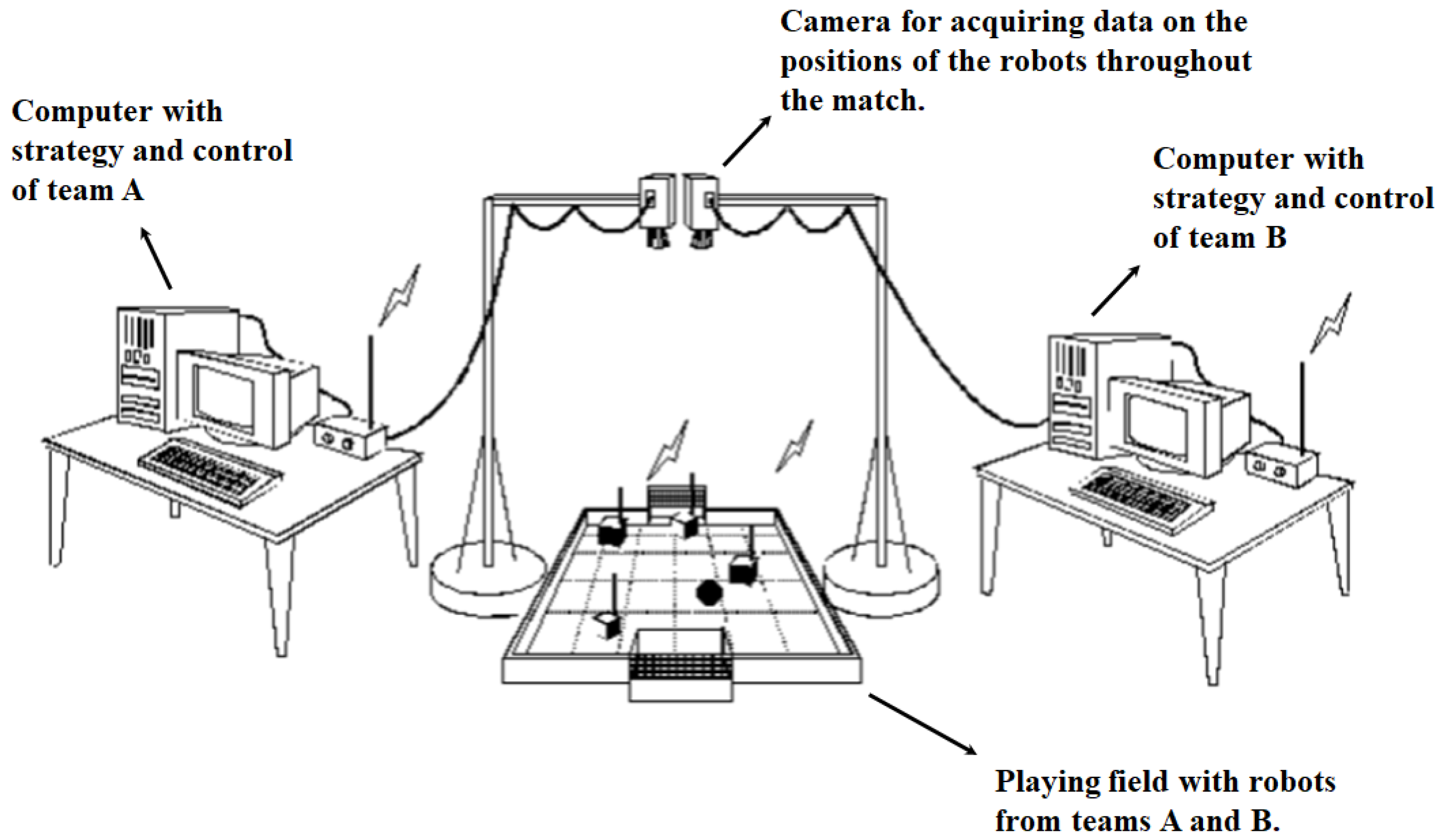
2. Structure of the Competitions

Figure 2 presents the official structure used for robot soccer matches. This structure has a camera that is responsible for capturing data about the robots, a remote communication system for sending information to the robots, computers for image processing and execution of the control algorithm, and a base area for robot locomotion [31].

2.1. Computer Vision

Through a camera present on the plane where the match takes place, it is possible to identify the position and orientation of a given robot in the field through image treatment performed by a computational algorithm. Each robot in the field has colored tags, as can be seen in Figure 1, whose function is to help the image algorithm to determine which team each robot belongs to, what its role on the field is, and, especially, its orientation, which is of great importance to control the robots [32,33].

The first step of the algorithm is to search for pixels with the same color as each team; these pixels are transformed into large regions of white color called “Blobs”. Then, the first step is performed again, but for the individual colors of each robot. In this way, the algorithm searches for the “Blobs” of individual colors closest to the “Blobs” that have the team color to identify which are the allied robots. Furthermore, a function calculates the midpoint between these “Blobs”, making it possible to draw a line between these two points, with the center of the line considered to be the central position of the robot. The robot’s position is given by the location of the central point of the line in a Cartesian plane that is traced over the entire extension of the field where the match takes place [33,34].

2.2. Communication and Triggering

Each robot has an ESP32 microcontroller with a Bluetooth transceiver that is responsible for receiving control signals remotely from the computer that is executing the control algorithm. In the microcontroller, the control signals are converted into PWM signals to drive an H-bridge converter, which is a circuit used in power electronics to allow the inversion of polarity and to control the magnitude of current in a load. This circuit allows the robot to activate the movement of the DC motors coupled to the wheels and, consequently, to move forwards and backwards, considered in this work as the positive and negative directions, respectively [35]. The DC motors used in the robot, which are shown in Figure 3, are from the 6 V Pololu brand and have a gearbox capable of converting the speed developed at the motor shaft at a ratio of 30:1 at the tip of the gearbox shaft; the motors have a maximum speed of 1100 RPM without load and provide a torque of 0.45 kg·cm.

This choice was based on the motor’s ability to provide adequate torque and satisfactory speed, allowing the robot to be fast without compromising the torque required for efficient movement. Furthermore, a significant advantage of this model is its small size, which helps to optimize the robot’s internal space, ensuring better integration with other components. With this choice, we seek to balance performance and efficiency in a compact and effective engine.

The low-level implementation code is responsible for configuring the peripherals used in the ESP32 in addition to having a programmed control strategy for controlling the speed of the robot’s wheel motors, which is necessary, as without this implementation, there is no guarantee that the speeds received by the computer via Bluetooth are achieved. The implemented speed control strategy for the robot’s wheel motors is done in a closed loop, thus, we obtain the speed value in RPM as feedback through encoders. The encoder used is of the magnetic type and uses the Hall effect, has a 6-pole magnetic disc, and provides a resolution of 12 counts per shaft rotation [10].

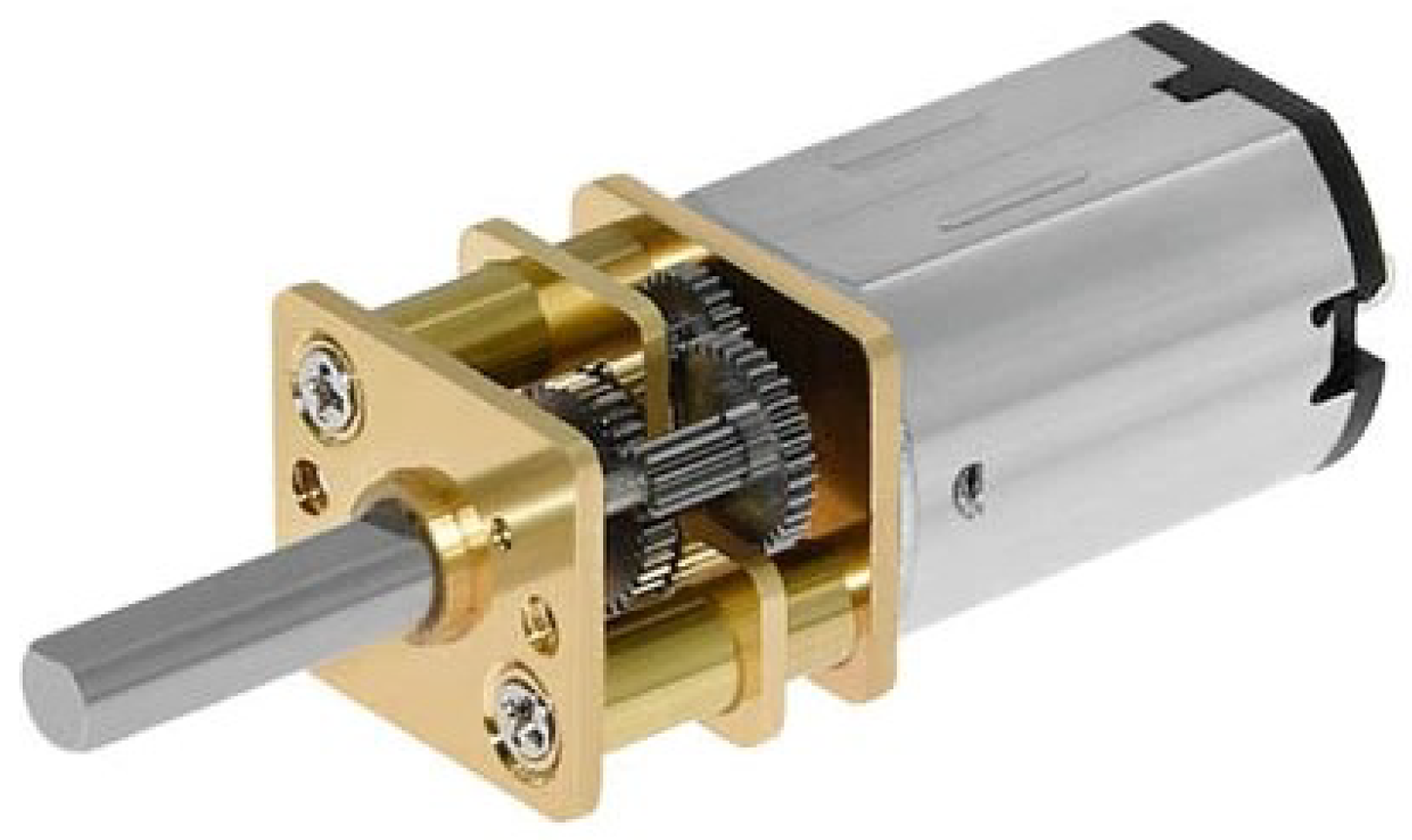
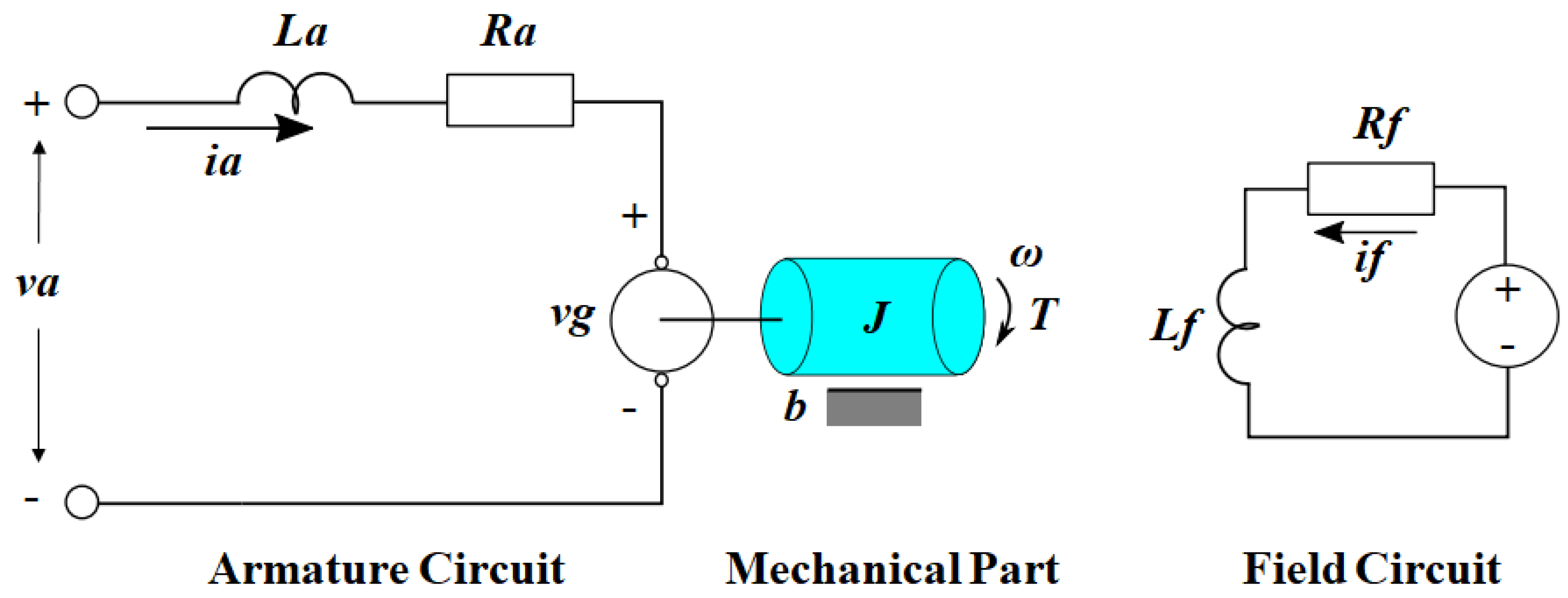
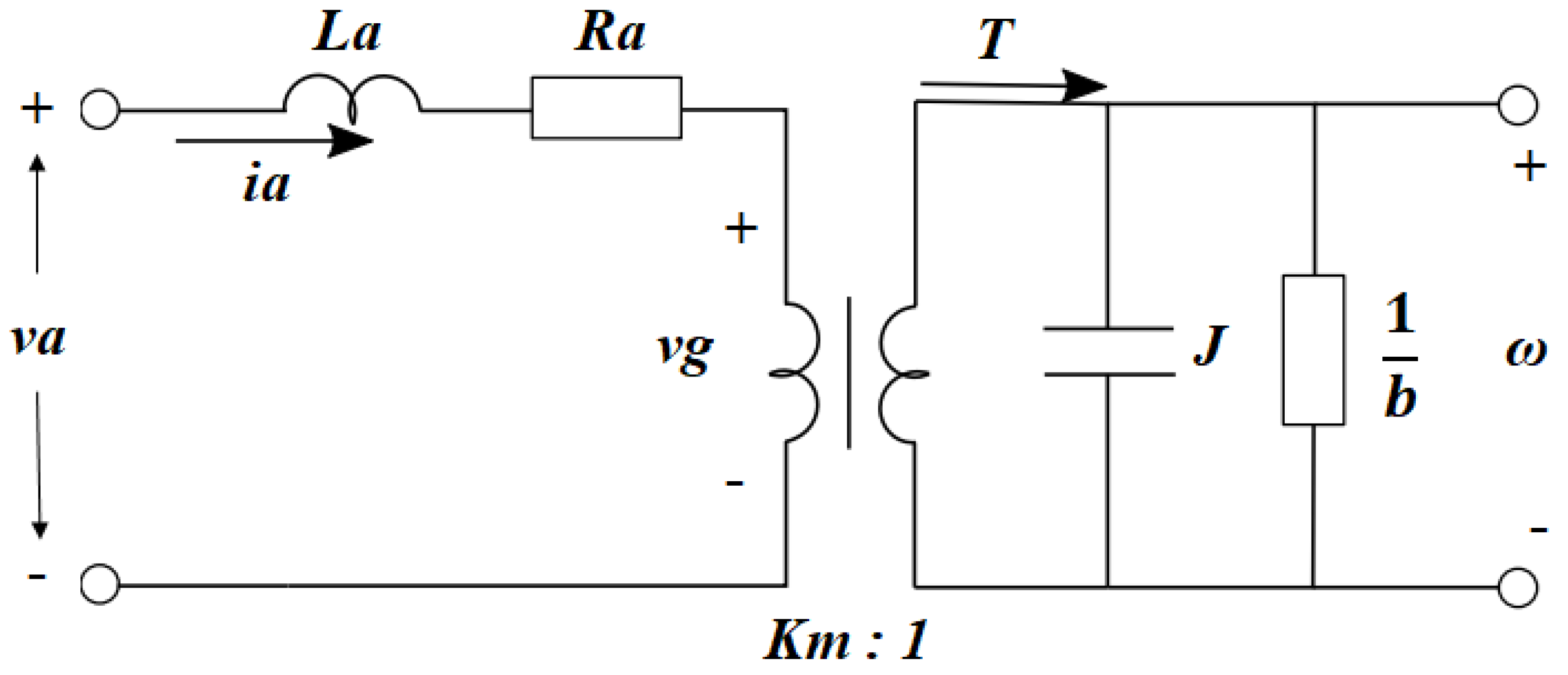
3. DC Motor Mathematical Modeling

Many applications using miniature DC motors require the motors to be driven at more than one load point or through specific load cycles. Running the motor at usable load points requires an adjustable power supply, which can be achieved by adjustable DC voltage supplies or by pulse-width modulation (PWM). PWM voltage regulation can be used effectively in battery- or direct-current-source-driven applications. Improved PWM drive efficiency increases battery life and reduces the heating of electronic components. DC motors offer very little inertia and low inductance. This allows the use of the engine in an application where dynamic behavior and fast responses are desired. The use of PWM allows current control in the windings. Therefore, the output angular speed, which is linearly proportional to the average winding current, can be controlled correctly [36].

A DC motor basically consists of the armature winding, field winding or permanent magnets, commutator, and brushes, for which:

• Armature winding: it is located in the rotating part of the DC motor (rotor) and is responsible for producing the torque that moves it and the output voltage when in generator mode.
• Field winding: this is a fixed part that is responsible for the constant magnetic flux passing through the armature; in small DC motors, such as those used in this work, the field winding is often replaced by placing permanent magnets around the armature, which are responsible for generating a constant magnetic field.
• Commutator: It keeps the armature current circulating in the same direction, causing the torque to maintain its direction for a constant input voltage.
• Brushes: these are where the armature winding contacts the power supply.

Direct current machines are widely used in control systems due to their linear behavior. Figure 4 shows a schematic diagram of a DC machine (motor or generator).

Figure 4 presents a schematic diagram for a direct current (DC) motor controlled by the armature: that is, the input signal is the voltage applied to the armature ($va$) [37,38]. In this diagram, the load is being modeled by a moment of inertia J, and viscous friction is represented by the coefficient b. Therefore, it is considered that

$$vg=Km·\omega$$

(1)

and

$$T=Km·ia.$$

(2)

The constant $Km$ is known as the engine constant. Due to the relationships between the motor elements, it is possible to model the equivalent circuit of a DC motor, as shown in Figure 5.

From the circuit in Figure 5, the following transfer function is extracted:

$${\displaystyle \frac{\Omega \left(s\right)}{Va\left(s\right)}}={\displaystyle \frac{Km}{JLa{s}^2+(JRa+bLa)s+bRa+K{m}^2}}\left[{\displaystyle \frac{rad·s^{-1}}{V}}\right].$$

(3)

If the armature impedance is neglected ($La\to 0$)—which is almost always possible, as the time constant related to the mechanical behavior of the motor is much greater than that related to electrical operation—the function of transfer that relates the angular velocity at the output with the voltage input is represented by

$${\displaystyle \frac{\Omega \left(s\right)}{Va\left(s\right)}}={\displaystyle \frac{Km}{JRas+bRa+K{m}^2}}={\displaystyle \frac{K}{\tau s+1}}\left[{\displaystyle \frac{rad·s^{-1}}{V}}\right].$$

(4)

Therefore, if the armature impedance is neglected, the motor transfer function that relates the angular velocity to the input voltage behaves like a first-order system. The greatest difficulty encountered when controlling DC motors is the high amplitude of the armature current, which requires the use of an input signal $va$, which is provided by a high-power source [37,38]. Figure 6 presents the dynamic response to a step-type input for a first-order system.

From Figure 6, it is clear that the entry to the step begins at time $t_0$. The input signal has a minimum value ($u_{min}$) and a maximum value ($u_{max}$). The resulting output signal is initially at $y_0$, and once the step is applied, the output y tracks the input and eventually settles to its steady-state value $y_{ss}$. In this way, based on the input and output values of the system, it is possible to determine the value of the gain in steady-state, which is given by

$$K={\displaystyle \frac{\Delta y}{\Delta u}}={\displaystyle \frac{y_{ss}-y_0}{u_{max}-u_{min}}}.$$

(5)

To find the model time constant $\tau$, we must first determine where the output y should be for the time constant:

$$y\left(t_1\right)=0.632·y_{ss}+y_0.$$

(6)

Therefore, based on the output response of a first-order system to a step input, as shown in Figure 6, it is possible to determine the time $t_1$ that corresponds to the output value $y\left(t_1\right)$ of Equation (6) and thus obtain the value of the system’s time constant, which is given by

$$\tau =t_1-t_0.$$

(7)

Therefore, it is worth highlighting that this is the strategy used by the robotics team to obtain models of the motors attached to the robot’s wheels. As it is a simple strategy, it saves time and makes it easier to recalculate the parameters of each engine throughout a competition in case any maintenance or engine replacement actions are necessary. Thus, there is greater agility for tuning the gains of the controllers implemented in the low-level code responsible for controlling the speed of the robot’s wheels.

For the operation of the DC motors in the robots, voltage inputs proportional to the PWM percentage are applied. The motors are equipped with encoders used for speed control. Consequently, for each stage of the motors’ work cycle, the output response is obtained through the encoder.

With the input and output data, it is possible to obtain mathematical models for the design of local controllers. A total of eight local models are established for different PWM input voltage levels.

4. Control Strategies

4.1. Local Discrete PI Controllers

After performing mathematical modeling and obtaining the respective models for different operating points, local discrete PI controllers using the root locus technique were designed. This gain-tuning technique involves modifying the root locus by adding poles and zeros to the open-loop transfer function of the system. This allows for shifting the roots to the desired closed-loop poles in the frequency domain [12].

A characteristic of this method is that it assumes the presence of a pair of dominant poles in the closed circuit based on the choice of a value for the overshoot and settling time ($t_s$). Therefore, the addition of zeros and poles does not significantly influence the characteristics of the response, and this technique then consists of modifying the location of the roots of the mathematical model using a compensator so that a pair of dominant closed-loop poles can be placed in the position desired [39].

To tune and design the gains of a discrete PI controller using the root locus method, firstly, from the local models obtained for the motors’ operating ranges, it was necessary to discretize the models for a sampling period T, which was chosen to respect the processing time of the ESP32 microcontroller used to build the robots. For discretization, the ZOH (zero-order hold) method was used, which works as a D/A converter and can memorize the last sample of the signal until a new input is inserted into the system.

To design the controller in the z domain, it is necessary to define an overshoot and a settling time. When starting the calculations, it is desired to determine the damping coefficient ($\zeta$), which can be obtained by

$$\zeta =\sqrt{{\displaystyle \frac{l{n}^2\left(overshoot\right)}{l{n}^2\left(overshoot\right)+{\pi }^2}}}.$$

(8)

Furthermore, to obtain the desired pair of poles ($z_d$) in the z plane, it is necessary to obtain the system’s undamped natural oscillation frequency ($w_n$), the damped oscillation frequency ($w_d$), and the frequency of natural sampling ($w_s$), which are presented, respectively, by

$$w_n={\displaystyle \frac{4}{t_s·\zeta }},$$

(9)

$$w_d=w_n·\sqrt{1-{\zeta }^2}$$

(10)

and

$$w_s={\displaystyle \frac{2\pi }{T}}.$$

(11)

In this way, it is possible to obtain the desired pole, which is given by

$$z_d=\left|z_d\right|·e^{j\angle z_d}$$

(12)

in which

$$|z_d|=e^{-\zeta ·w_n·T}$$

(13)

and

$$\angle z_d={\displaystyle \frac{2·\pi ·w_d}{w_s}}.$$

(14)

Considering

$$X+jY={\displaystyle \frac{-1}{G\left(z_d\right)}}$$

(15)

and

$$\alpha +j\beta ={\displaystyle \frac{z_d·T}{z_d-1}}$$

(16)

with X and $\alpha$ being the real part and Y and $\beta$ being the imaginary part of Equations (15) and (16), respectively, we have that

$$Kp=X-{\displaystyle \frac{\alpha ·Y}{\beta }}$$

(17)

and

$$Ki={\displaystyle \frac{Y}{\beta }}.$$

(18)

In this way, from the gains calculated via the discrete root locus method, it is possible to determine the transfer function of each local controller $C\left(z\right)$, which is given by

$$C\left(z\right)={\displaystyle \frac{U\left(z\right)}{E\left(z\right)}}={\displaystyle \frac{(Kp+Ki·T)z-Kp}{z-1}},$$

(19)

making it possible to determine the difference equation for each local controller, which is then implemented in the low-level code for effective speed control of the motors coupled to the right and left wheels of the robot [40].

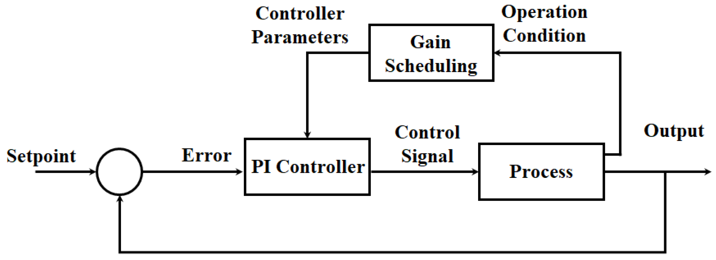
4.2. Gain Scheduling Control

The control performed by gain scheduling originated in the development of flight control systems and is considered an adaptive system, i.e., a controller that can modify its behavior in response to changes in the process dynamics and disturbance characteristics—it is a model capable of adapting quickly [41,42]. It is classified as a feedback control system, in which gains are adjusted using feedforward compensation [43].

The key point in developing this method is to determine the auxiliary variables that have a good correlation with changes in the process dynamics. Figure 7 represents the logic for the implementation of a gain scheduler.

Therefore, by changing the parameters to be functions of auxiliary variables, it is possible to obtain the best adaptation of the compensator to different operating conditions of the plant. The following steps make it possible to implement a gain scheduler:

• Obtain a valid representation or approximation of the nonlinear system for each operating point and perform its linearization;
• Apply linear control techniques to develop a controller that meets the needs of the linearized system;
• Choose the architecture of the gain scheduler (rules used in transitions);
• Validate the performance of the controller.

It is important to note that gain scheduling is open-loop compensation, so there is no feedback to correct incorrect programming. Additionally, it is worth emphasizing the abundance of operating conditions that must be analyzed to determine the controller’s parameters.

The main advantage of applying this technique is its rapid response to changes in the process. Since there is no estimation of parameters, only selection structures, the limiting factors depend solely on the response speed of the auxiliary measurements to changes in the process [44,45].

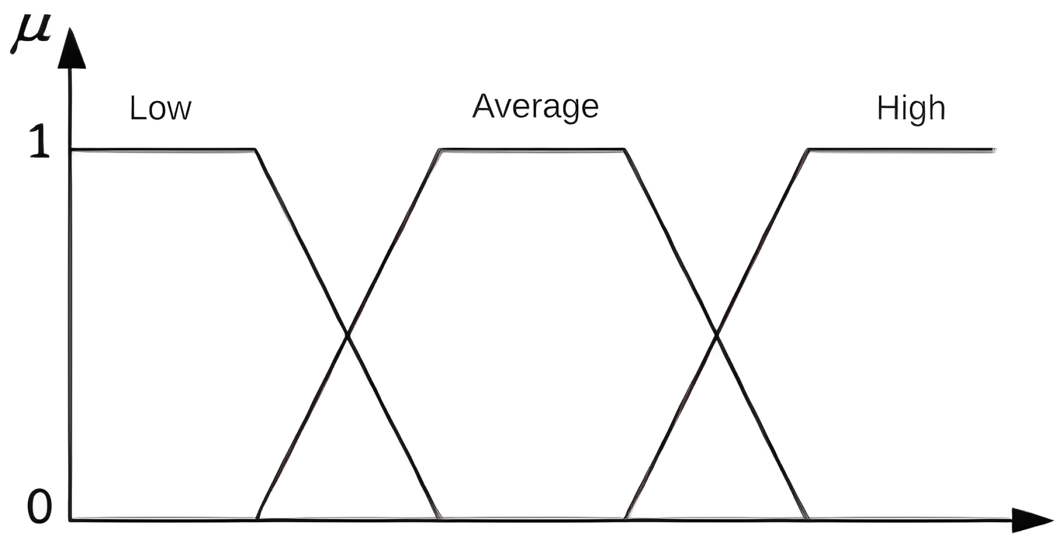
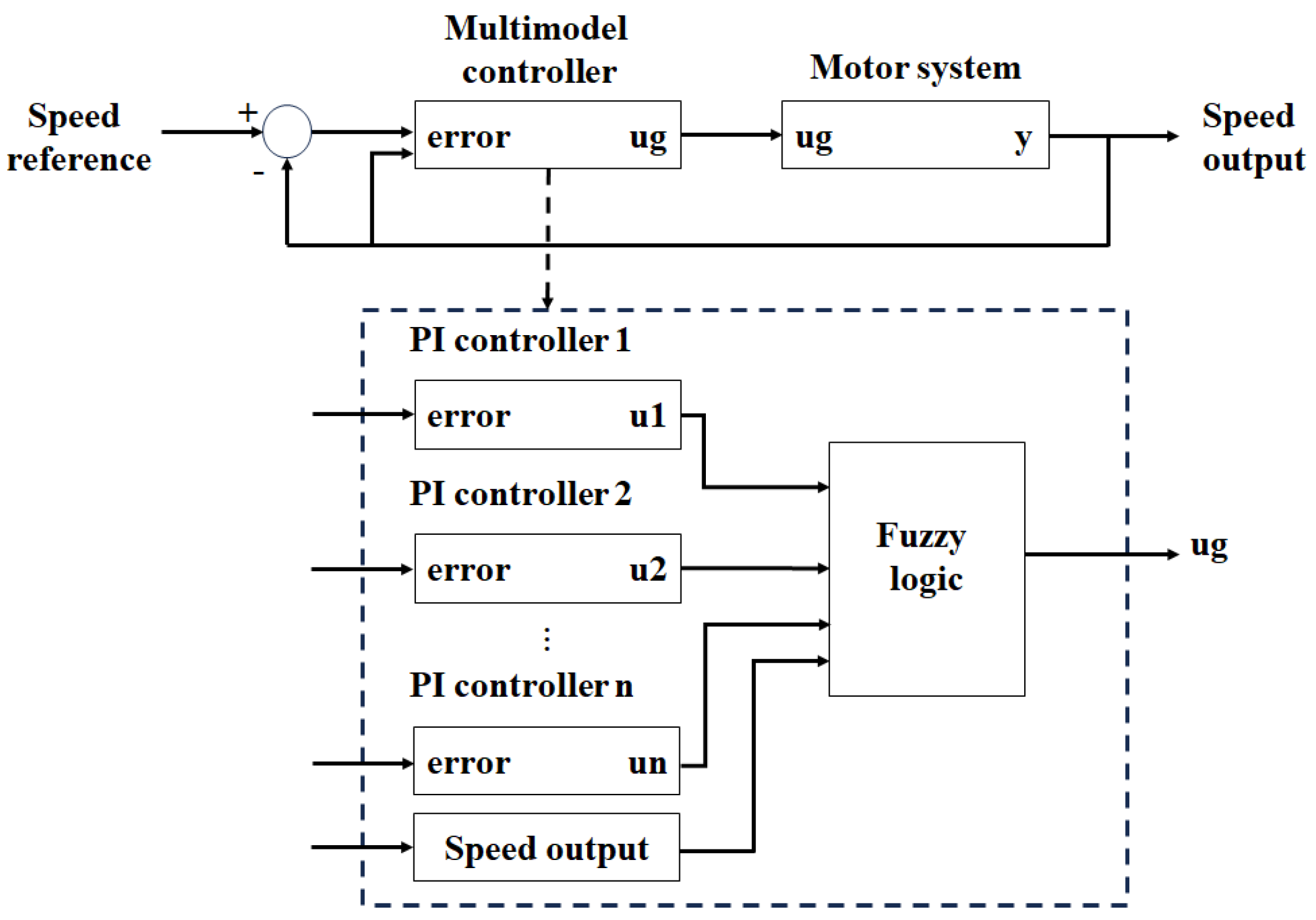
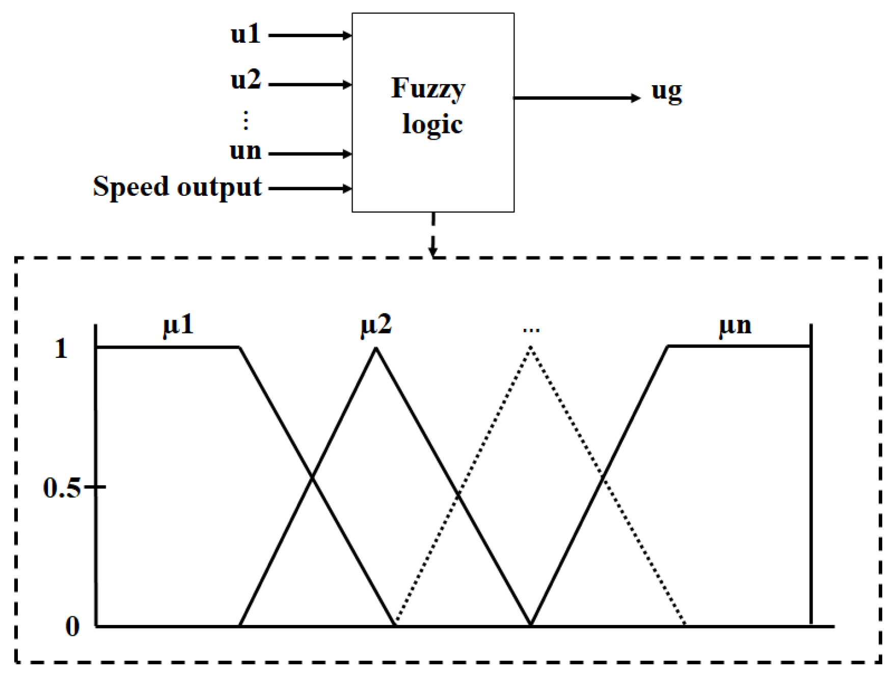
4.3. Fuzzy Multimodel Control

A fuzzy set is defined as a set of objects whose degree of membership is relative to the continuous interval between 0 and 1. Thus, within the operating range, fuzzy membership functions (numeric, graphical, or tabular) are applied to assign fuzzy membership values to the control variable. Trapezoidal, triangular, and Gaussian functions are most commonly used in the literature [46,47]. Figure 8 shows an example of trapezoidal membership functions.

Therefore, fuzzy system inferences involve evaluating rules that describe the dependence between input and output variables. Two concepts are widely used for developing fuzzy systems: fuzzification and defuzzification. Fuzzification involves converting real-world quantities into fuzzy numbers, which can come from sensors or computerized systems, among other sources [47].

The system rules are treated in parallel. Therefore, when an input is provided, different rules with their respective degrees of activation are triggered to infer a control signal. This combination of different rules is called defuzzification [48].

The work aims to develop a nonlinear control system through a multimodel control strategy using local discrete-time PI controllers linked by fuzzy logic. The use of fuzzy logic is because its models are universal approximators of functions in a compact space [49]. Fuzzy models also allow the composition of the global model from multiple local models, which is advantageous for interpretability and controller design.

With the development of local controllers for the desired operating points, these can be combined via fuzzy logic so that the application is no longer local, meaning the system is controlled globally. This union favors the application of multimodel hybrid control over a wide operating range, making local PI controllers in discrete time act on the global process plant through the degree of the relevance of local controllers to each operating region [50].

This degree of pertinence is calculated by functions that represent the operating ranges, and, via IF–THEN rules, the output signal, which acts on the global process plant, is determined. To implement the multimodel control strategy, the first step is to obtain the discrete-time PI controllers for each linearized operating point. After obtaining the local controllers, it is necessary to choose the fuzzy rules that will unite all local controllers through the developed fuzzy membership functions, as shown in Figure 9 and Figure 10.

Figure 9 shows that each local controller generates its own control signal that acts best close to its operating point. Now, from Figure 10, it can be seen that each local control signal presents a membership function with a corresponding degree of membership $\mu$, so that

$$\left\{\begin{array}{c}u1\mathrm{will}\mathrm{have}\mathrm{a}\mathrm{membership}\mathrm{degree}\mu 1\hfill \\ u2\mathrm{will}\mathrm{have}\mathrm{a}\mathrm{membership}\mathrm{degree}\mu 2\hfill \\ ⋮\hfill \\ un\mathrm{will}\mathrm{have}\mathrm{a}\mathrm{membership}\mathrm{degree}\mu n\hfill \end{array}\right.$$

In this way, depending on the reference position to be tracked, each local controller provides a respective value of the control signal, represented by a function $u\left(k\right)$, so that the local controller’s performance is represented by its respective degree of membership $\mu$, which is used to activate the fuzzy rules. With activation of the fuzzy rules, the calculation of the output signal due to the action of the membership functions is obtained.

Based on the response of the system to be controlled and the output of the local models, linear controllers act on each local model in order to correct the response of each model separately. Global control action is obtained by fuzzy inference, which in this case is a combination weighted by the fuzzy mode for the actions of each local PI discrete-time controller. The global control signal excites the motor system to act on the reference position. In this way, global control action is obtained by

$$ug={\displaystyle \frac{{\sum }_{i=1}^n\mu i·ui}{{\sum }_{i=1}^n\mu i}}$$

(20)

where $\mu i$ is the activation value of the i-th rule (local model), $ui$ the control action determined by the i-th controller, and i is the number of local models/controllers.

Thus, with the union of all local controllers developed, based on linear models together with fuzzy logic implemented through IF–THEN rules, an output signal is obtained, which acts on the system to maintain tracking of the input reference with the desired dynamic characteristics.

5. Results

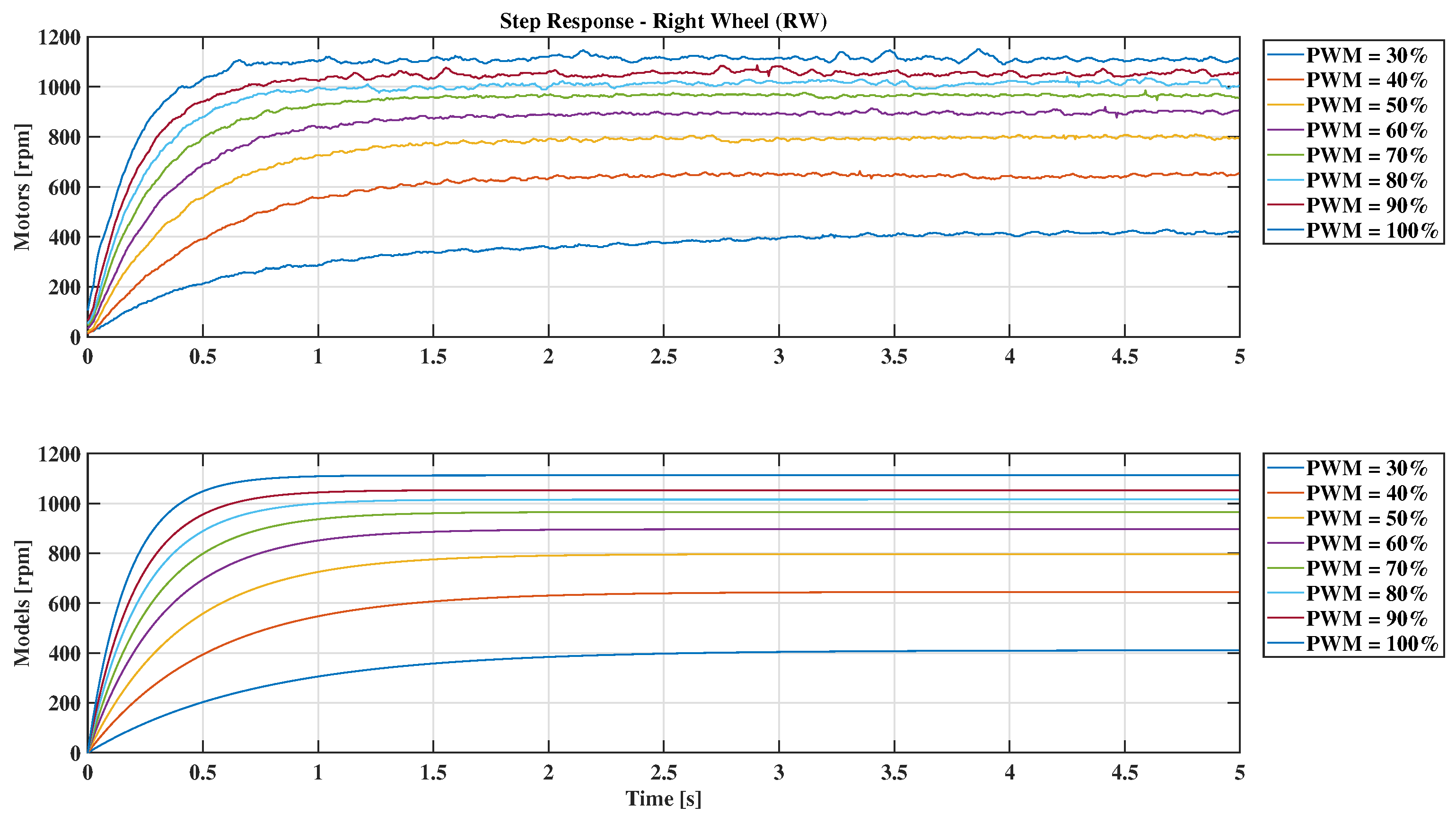
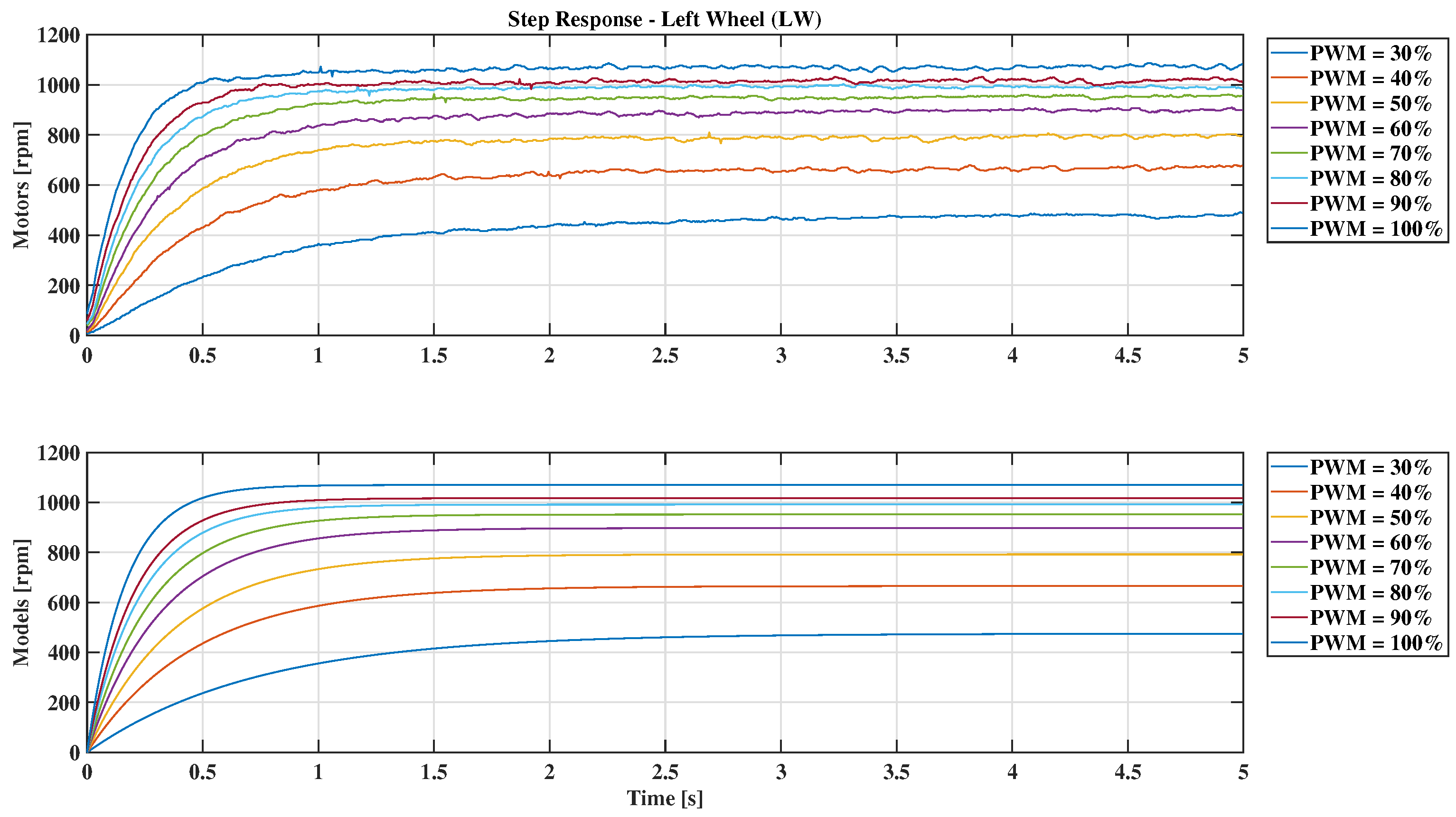
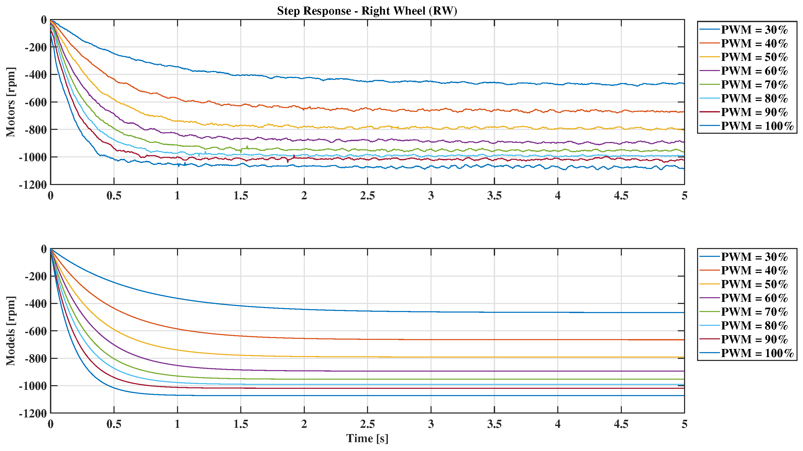
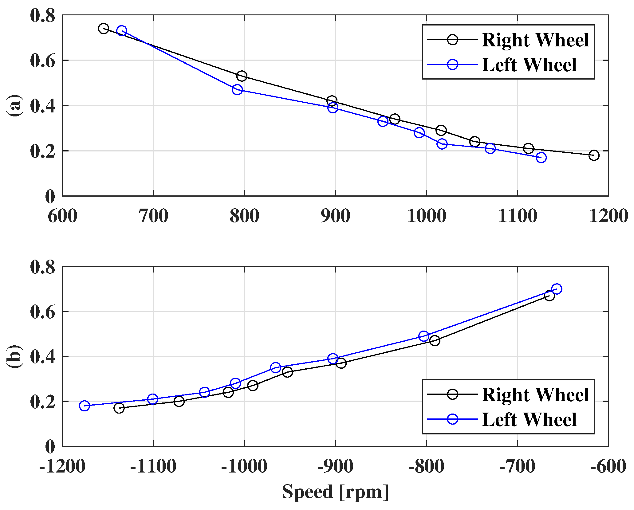
5.1. Local Models and PI Controllers

Initially, a code for open-loop tests was implemented in the ESP32 microcontroller code with the purpose of performing data acquisition for the entire PWM range applied to the motor input. Figure 11 and Figure 12 present the acquired data and the validation of the models obtained for ranges from 30% to 100% for the PWM of the right and left wheel motors, respectively, in the positive direction of the trajectory: that is, considering that the robot is moving forward. It is noted that the motors are coupled to the wheels, and in the positive direction, they have an open-loop rotation difference, meaning that the robot does not walk in a straight line.

Figure 13 and Figure 14 present the acquired data and the validation of the models obtained for ranges from 30% to 100% of the PWM for the right and left wheel motors, respectively, in the negative direction of the trajectory: that is, considering that the robot is moving backwards. It is noted that the motors are coupled to the wheels, and for the negative direction, they also have an open-loop rotation difference, meaning that the robot does not walk in a straight line.

Due to the need to make the robot able to follow a straight trajectory, it is necessary to implement controllers to achieve this objective. So for this work, discrete local controllers were developed to meet the following operating criteria: maximum overshoot of 1%, sampling time of 5 ms, and settling time equivalent to 4 times $\tau$.

Table 1. Models of the right wheel (RW) and left wheel (LW) and their respective gains (Kp and Ki).

Positive Direction
PWM Step (%)	RW Model	Kp	Ki	LW Model	Kp	Ki
30	${\displaystyle \frac{13.70}{0.74s+1}}$	0.754	4.85	${\displaystyle \frac{15.84}{0.73s+1}}$	0.643	4.14
40	${\displaystyle \frac{16.12}{0.53s+1}}$	0.446	2.98	${\displaystyle \frac{16.64}{0.47s+1}}$	0.377	2.56
50	${\displaystyle \frac{15.94}{0.42s+1}}$	0.340	2.36	${\displaystyle \frac{15.84}{0.39s+1}}$	0.313	2.20
60	${\displaystyle \frac{14.94}{0.34s+1}}$	0.280	2.04	${\displaystyle \frac{14.96}{0.33s+1}}$	0.269	1.97
70	${\displaystyle \frac{13.79}{0.29s+1}}$	0.248	1.88	${\displaystyle \frac{13.60}{0.28s+1}}$	0.240	1.84
80	${\displaystyle \frac{12.69}{0.24s+1}}$	0.215	1.72	${\displaystyle \frac{12.39}{0.23s+1}}$	0.208	1.69
90	${\displaystyle \frac{11.70}{0.21s+1}}$	0.194	1.64	${\displaystyle \frac{11.29}{0.21s+1}}$	0.194	1.66
100	${\displaystyle \frac{11.12}{0.18s+1}}$	0.156	1.44	${\displaystyle \frac{10.69}{0.17s+1}}$	0.147	1.41
Negative Direction
PWM Step (%)	RW Model	Kp	Ki	LW Model	Kp	Ki
30	${\displaystyle \frac{15.54}{0.67s+1}}$	0.680	3.19	${\displaystyle \frac{14.29}{0.70s+1}}$	0.643	3.62
40	${\displaystyle \frac{16.62}{0.47s+1}}$	0.377	2.11	${\displaystyle \frac{16.43}{0.49s+1}}$	0.400	2.22
50	${\displaystyle \frac{15.81}{0.37s+1}}$	0.294	1.72	${\displaystyle \frac{16.07}{0.39s+1}}$	0.313	1.81
60	${\displaystyle \frac{14.89}{0.33s+1}}$	0.271	1.63	${\displaystyle \frac{15.04}{0.35s+1}}$	0.289	1.71
70	${\displaystyle \frac{13.61}{0.27s+1}}$	0.234	1.49	${\displaystyle \frac{13.80}{0.28s+1}}$	0.242	1.52
80	${\displaystyle \frac{12.39}{0.24s+1}}$	0.214	1.42	${\displaystyle \frac{12.63}{0.24s+1}}$	0.216	1.43
90	${\displaystyle \frac{11.31}{0.20s+1}}$	0.180	1.30	${\displaystyle \frac{11.60}{0.21s+1}}$	0.196	1.36
100	${\displaystyle \frac{10.72}{0.17s+1}}$	0.154	1.19	${\displaystyle \frac{11.01}{0.18s+1}}$	0.157	1.20

represents each obtained mathematic model and the respective gains of each designed local controller.

Figure 15 shows the behavior of the time constant: that is, its evolution for each operating range of the mathematical models that were obtained to implement the controllers in this work. In this way, an adaptive control by gain scheduling and a fuzzy multimodel intelligent control were used so that the speeds of the robots’ wheels tracked a certain reference, allowing the robot to track a certain trajectory. To achieve this, the adjustments of each local controller occur according to the speeds of the motors for each PWM range.

Table 2. Speeds in RPM for selection of local controllers.

PWM (%)	Right Wheel (rpm)		Left Wheel (rpm)
	Positive	Negative	Positive	Negative
30	645	−665	665	−657
40	797	−791	792	−803
50	896	−894	897	−903
60	965	−953	952	−966
70	1016	−991	992	−1010
80	1053	−1018	1017	−1044
90	1112	−1072	1070	−1101
100	1184	−1138	1126	−1176

represents the speed of each operating point, which is used in the selection structures and was obtained through tachometer measurements.

The work was carried out in two stages: the first in a Simulink environment—a tool for modeling, simulating, and analyzing dynamic systems. Using the models and controllers developed and validated in the simulation environment, the second stage carried out a practical application on the robots.

The following subsections describe the responses obtained in the practical application. The results aim to represent the robot’s response to different speed references applied to it as well as the control signals applied to the motors. Various system performance criteria are adopted to define the best strategy to be employed.

Throughout the results, positive and negative references are depicted to represent the robot’s movement. In Figure 1, a positive reference corresponds to the robot’s forward movement towards the ball, while a negative reference represents its backward movement in the opposite direction of the ball. Furthermore, when performing an analysis between the results, it is observed that the control signals for the left and right wheels sometimes differ significantly. This occurs due to the presence of gearboxes in the motors, which demand higher control signals for the right wheel.

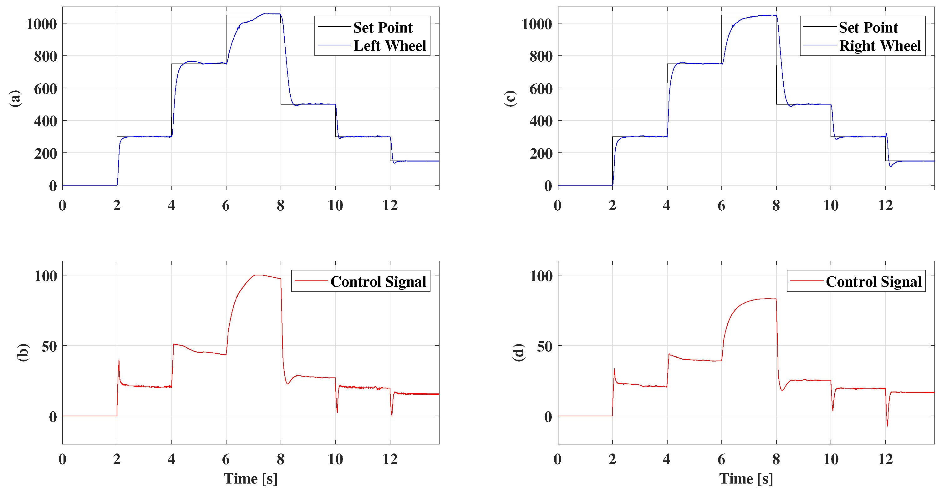
5.2. Gain Scheduling

The gain scheduling adaptive control technique can be considered to be a classic multimodel control strategy. Therefore, it is necessary to use a greater number of local controllers that can always be adjusted to the situations in which the system is inserted. Thus, the eight models obtained in the identification were used. Figure 16 represents the linear interpolation for the proportional and integral gains of the local controllers tuned for each model of the right wheels (represented in black) and the left wheels (in blue).

The control variables used were found by linear interpolation between the eight operating points. It is worth noting that saturations were placed for regions below the first operating point and regions above the last operating point.

Figure 17 shows the positive velocity tracking. It is possible to note that the adaptive gain scaling controller allowed a speed reference to be tracked. In this same figure, small overshoots can be observed. First, on the left wheel, close to 5 s, the wheel rotation speed reached a value of 764 rpm for the imposed reference of 700 rpm. The second overshoot can be seen for the right wheel after 10 s of testing, at which point the wheel rotation speed reached a value of 113 rpm for an imposed reference of 150 rpm. It is important to highlight that the control law was successful at handling these cases, and in both situations, these overshoots were corrected in less than half a second.

However, when analyzing Figure 18, which consists of applying the same method to track speed in the negative direction, performance that is not as good as that presented for the positive direction is observed. An underdamped response can be observed, meaning that the system behavior does not approach the speed reference smoothly but, rather, with oscillations. The system’s response to different speed references is much faster; however, more intense overshoots occur, and subsequently, oscillations with progressively decreasing amplitudes are observed until the speed tracking enters a steady state.

In this case, both wheels exhibit the most significant overshoot at the same point: around 2.5 s into the test and for a reference speed of −300 RPM. Observing Figure 18, at this point, the left wheel reaches a maximum speed of −406 RPM, while the right wheel reaches −382 RPM. The respective overshoots are 35% and 27%, indicating that the controller’s correction was not sufficient to prevent oscillatory behavior, impairing the robot’s performance in walking in a straight line.

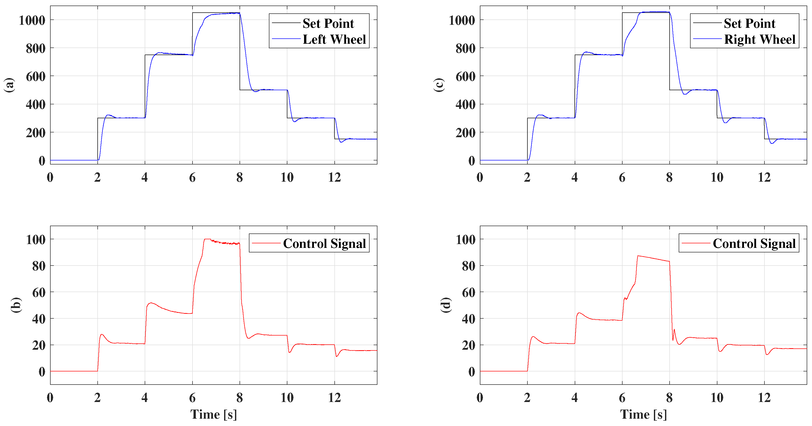
5.3. Fuzzy Multimodel Control with Two Models

This approach involves obtaining a controller that provides a global control signal from the local 50% and 60% PWM models. When the speed reference is below 50% of PWM according to the values in Table 2, the local controller obtained for the 50% model is used, when the speed reference is above 60 %, the local controller developed for the 60% model is used. However, when the speed reference is at intermediate values between 50% and 60%, the fuzzy logic calculates the output based on the weights of the membership functions and fuzzy rules. Figure 19 presents the result of the dynamics of the right and left wheels of the robot and the control signal for changes in the reference considering the positive direction, and Figure 20 shows changes in the reference considering the negative direction.

From Figure 19, just after 6 s, the fuzzy inference between the local controllers is noticeable, as the output dynamics present different dynamic behavior, as observed in the speed curves for the (a) left wheel and (c) right wheel. Additionally, around 6.5 s, a switch to the 60% PWM controller is noticed for both wheels. As this technique uses only two models, the controllers may not be well-adjusted to reference speeds far from their operating points, causing the engine system to present the desired dynamic behavior.

In Figure 20, there is a fuzzy inference happening between the local controllers at a time close to 6 s. The behavior is the same when compared to the positive direction: that is, for operating points far from the local controllers used, there is a greater number of overshoots and unwanted dynamic behavior. It is important to highlight that even when the controllers are not well-adjusted for speeds far from their operating points, tracking of the input reference is maintained.

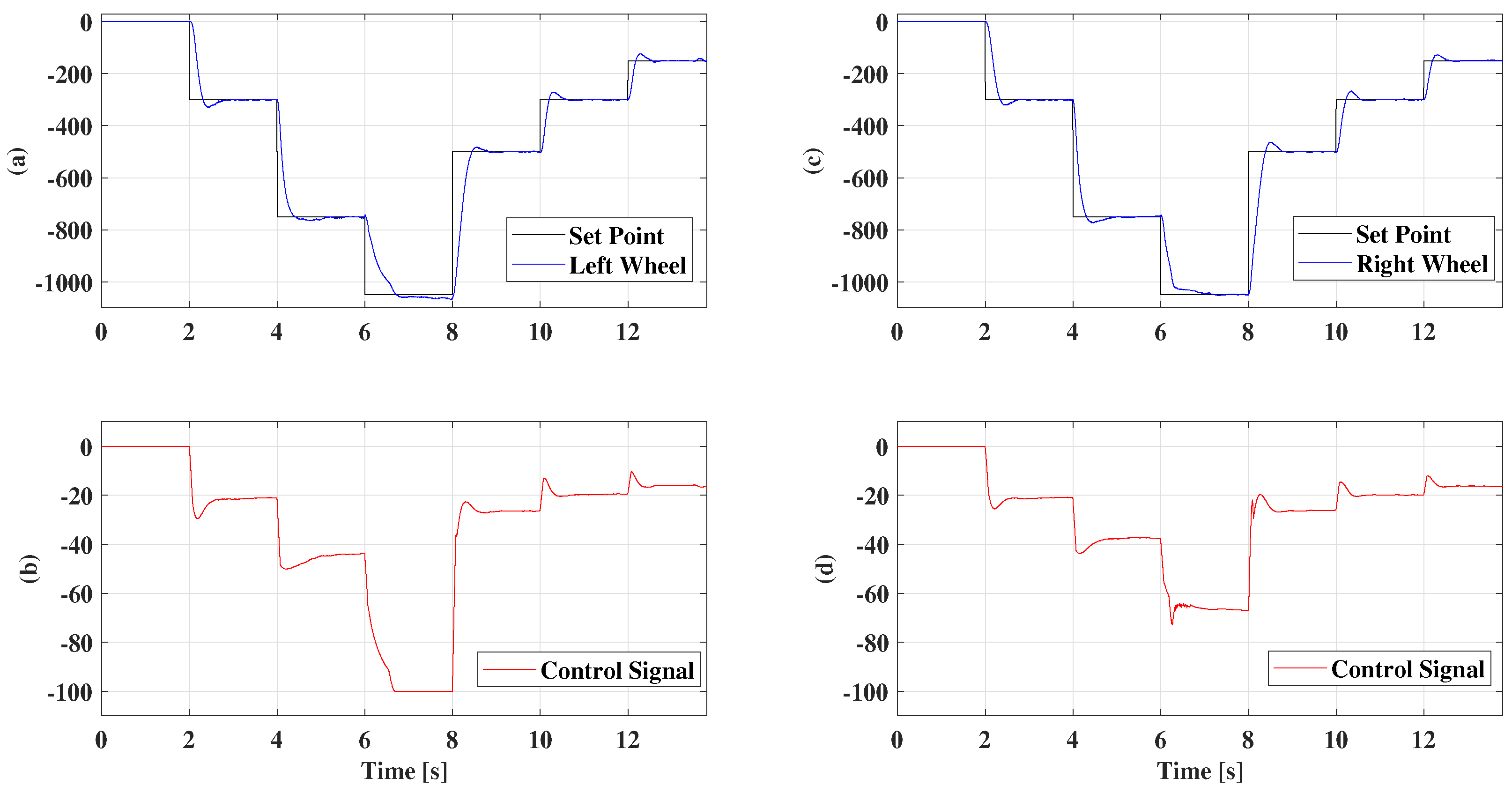
5.4. Fuzzy Multimodel Control with Three Models

This approach involves obtaining a controller that provides a global control signal starting from the local 30%, 60%, and 90% PWM models. When the speed reference is below 30% of PWM according to the values in Table 2, the local controller obtained for the 30% model is used; when the speed reference is above 90 %, the local controller developed for the 90% model is used. However, when the speed reference is at intermediate values between 30%, 60%, and 90%, the fuzzy logic calculates the output based on the weights of the membership functions and fuzzy rules. Figure 21 presents the result of the dynamics for the right and left wheels of the robot and the control signal for changes in the reference considering the positive direction, and Figure 22 shows changes in the reference considering the negative direction.

From Figure 21 and Figure 22, it can be seen that the input reference tracking was maintained for both the right wheel motor and the left wheel. Furthermore, it is noted that the control signal applied to the motors is within the acceptable PWM percentage range based on the drive electronics developed for the robot wheel motors.

5.5. Fuzzy Multimodel Control with 4 Models

This approach involves obtaining a controller that provides a global control signal starting from the local 30%, 50%, 70%, and 90% PWM models. When the speed reference is below 30% of PWM according to the values in Table 2, the local controller obtained for the 30% model is used; when the speed reference is above 90 %, the local controller developed for the 90% model is used. However, when the speed reference is at intermediate values between 30%, 50%, 70%, and 90%, the fuzzy logic calculates the output based on the weights of the membership functions and fuzzy rules. Figure 23 presents the result of the dynamics of the right and left wheels of the robot and the control signal for changes in the reference considering the positive direction, and Figure 24 shows changes in the reference considering the negative direction.

Similarly, from Figure 23 and Figure 24, it can be seen that the tracking of the input reference was maintained for both the right wheel motors and the left wheel. Furthermore, it is noted that the control signal applied to the motors is within the acceptable PWM percentage range based on the drive electronics developed for the robot wheel motors.

5.6. Performance Criteria

As previously noted, each controller presented satisfactory performance in tracking the imposed reference and providing a control signal within acceptable parameters for the electronics developed to drive the motors. Therefore, two performance criteria were used to characterize the performance of each control system: ISE (integral square error) and ITAE (integral of time multiplied absolute error). The objective of using both criteria is their complementarity. ISE is based on quadratic error and penalizes more significant errors at the beginning of the response. On the other hand, ITAE is based on weighted error over time and penalizes errors that persist for more extended periods.

Table 3. Performance criteria for the right wheel in positive and negative directions.

Right Wheel
	Positive Direction		Negative Direction
	ISE	ITAE	ISE	ITAE
Gain Scheduling	$5.517\times {10}^4$	$2.516\times {10}^3$	$4.355\times {10}^4$	$2.241\times {10}^3$
Multimodel Control: 2 Models	$8.728\times {10}^4$	$3.188\times {10}^3$	$6.270\times {10}^4$	$2.521\times {10}^3$
Multimodel Control: 3 Models	$3.583\times {10}^4$	$2.049\times {10}^3$	$3.192\times {10}^4$	$1.956\times {10}^3$
Multimodel Control: 4 Models	$5.096\times {10}^4$	$2.599\times {10}^3$	$3.395\times {10}^4$	$2.033\times {10}^3$

and

Table 4. Performance criteria for the left wheel in positive and negative directions.

Left Wheel
	Positive Direction		Negative Direction
	ISE	ITAE	ISE	ITAE
Gain Scheduling	$6.557\times {10}^4$	$2.574\times {10}^3$	$4.489\times {10}^4$	$2.511\times {10}^3$
Multimodel Control: 2 Models	$7.955\times {10}^4$	$2.863\times {10}^3$	$7.240\times {10}^4$	$2.723\times {10}^3$
Multimodel Control: 3 Models	$5.725\times {10}^4$	$2.425\times {10}^3$	$4.415\times {10}^4$	$2.142\times {10}^3$
Multimodel Control: 4 Models	$6.261\times {10}^4$	$2.581\times {10}^3$	$4.447\times {10}^4$	$2.211\times {10}^3$

present the errors obtained for each criterion for the right and left wheels, respectively.

Calculating the average values between the right and left wheels and considering both positive and negative tracking, the result is the same for both criteria: the fuzzy multimodel intelligent controller with the models presents the criteria with the lowest errors. This shows that the fact that a fuzzy multimodel intelligent controller is developed to take into account a greater number of models does not mean that it will have better performance. Furthermore, the technique is an alternative to solutions in which there is a variety of models that represent the dynamics of the system at different operating points. The choice of the number of models obtained is at the discretion of the designer, because although there is no direct relationship between the performance and the number of models, the technique allows the tracking of an imposed reference, enabling the control of the robot’s wheel motors and, consequently, helping to control the robot’s dynamics throughout a football match.

6. Conclusions

The objective of this work was to implement and compare the performance of the adaptive control strategy by gain scheduling and the fuzzy multimodel intelligent control strategy for tracking the speed of the wheels of non-holonomic robot motors with differential drive used in robot football competitions. The comparison was made between adaptive control by scaling gains and intelligent controllers considering two, three, and four models for the tuning and design of local controllers. For the fuzzy multimodel intelligent controller, the global control signal is derived from a fuzzy inference of PI controllers that are designed for each obtained and chosen local model.

The results demonstrate that the choice of a multimodel approach was successful, especially in fuzzy logic applications. This allowed the system to track all speed steps used as references from a smooth change between signals from each local controller, which is impossible in the gain scheduling strategy. Furthermore, it allowed the team’s robot to work with the entire speed range, which was not possible before. Notably, all implementations presented satisfactory results, with good response times and rapid convergence to the reference. Each method has its main positive and negative characteristics. However, based on the performance criteria analyzed, the multimodel fuzzy controller with three models proved to be the most efficient for application to the studied robot. It achieved the lowest errors regarding positive and negative wheel speeds in all possible scenarios.

Therefore, the objective of this work to assist the robotics team at the Federal University of Itajuba, Campus Itabira, with solving the speed control problem was fulfilled, and in this way, the team can provide greater competitiveness in the competitions they compete in. Furthermore, this work can provide a basis for advanced control strategies to be explored in academic and research settings among team members.

References

1. Niku, S.B. Introduction to Robotics: Analysis, Control, Applications; John Wiley & Sons: Hoboken, NJ, USA, 2020. [Google Scholar]
2. Siegwart, R.; Nourbakhsh, I.R.; Scaramuzza, D. Introduction to Autonomous Mobile Robots; MIT Press: Cambridge, MA, USA, 2011. [Google Scholar]
3. Bruzzone, L.; Nodehi, S.E.; Fanghella, P. Tracked locomotion systems for ground mobile robots: A review. Machines 2022, 10, 648. [Google Scholar] [CrossRef]
4. Sun, W.; Tang, S.; Gao, H.; Zhao, J. Two timescale tracking control of nonholonomic wheeled mobile robots. IEEE Trans. Control Syst. Technol. 2016, 24, 2059–2069. [Google Scholar] [CrossRef]
5. Rubio, F.; Valero, F.; Llopis-Albert, C. A review of mobile robots: Concepts, methods, theoretical framework, and applications. Int. J. Adv. Robot. Syst. 2019, 16, 1729881419839596. [Google Scholar] [CrossRef]
6. De Wit, C.C.; Sordalen, O. Exponential stabilization of mobile robots with nonholonomic constraints. In Proceedings of the [1991] 30th IEEE Conference on Decision and Control, Brighton, UK, 11–13 December 1991; IEEE: Piscataway, NJ, USA, 1991; pp. 692–697. [Google Scholar]
7. Chen, Z.; Liu, Y.; He, W.; Qiao, H.; Ji, H. Adaptive-neural-network-based trajectory tracking control for a nonholonomic wheeled mobile robot with velocity constraints. IEEE Trans. Ind. Electron. 2020, 68, 5057–5067. [Google Scholar] [CrossRef]
8. Bie, H.; Li, P.; Chen, F.; Ghaderpour, E. An Observer-Based Type-3 Fuzzy Control for Non-Holonomic Wheeled Robots. Symmetry 2023, 15, 1354. [Google Scholar] [CrossRef]
9. Cen, H.; Singh, B.K. Nonholonomic wheeled mobile robot trajectory tracking control based on improved sliding mode variable structure. Wirel. Commun. Mob. Comput. 2021, 2021, 1–9. [Google Scholar] [CrossRef]
10. Akande, T.; Alabi, O.; Ajagbe, S. A deep learning-based CAE approach for simulating 3D vehicle wheels under real-world conditions. Artif. Intell. Appl. 2024. [Google Scholar] [CrossRef]
11. Sani, M.; Hably, A.; Robu, B.; Dumon, J.; Meslem, N. Real-time Dynamic Obstacle Avoidance for a Non-holonomic Mobile Robot. In Proceedings of the 2023 IEEE 32nd International Symposium on Industrial Electronics (ISIE), Helsinki/Espoo, Finland, 19–21 June 2023; IEEE: Piscataway, NJ, USA, 2023; pp. 1–6. [Google Scholar]
12. Ogata, K. Modern Control Engineering; Prentice Hall: Upper Saddle River, NJ, USA, 2010. [Google Scholar]
13. Zin, T.P.; Nyein, A.K. DC Gear-Motor Position control for 3-DOF Articulated Painting Robot arm. In Proceedings of the International Conference on Science and Technology for Sustainable Development, Yangon, Myanmar, 7 August 2019. [Google Scholar]
14. Cook, M.D.; Bonniwell, J.L.; Rodriguez, L.A.; Williams, D.W.; Pribbernow, J. Low-cost dc motor system for teaching automatic controls. In Proceedings of the 2020 American Control Conference (ACC), Denver, CO, USA, 1–3 July 2020; IEEE: Piscataway, NJ, USA, 2020; pp. 4283–4288. [Google Scholar]
15. Sands, T. Control of DC motors to guide unmanned underwater vehicles. Appl. Sci. 2021, 11, 2144. [Google Scholar] [CrossRef]
16. Saá-Tapia, F.; Mayorga-Miranda, L.; Ayala-Chauvin, M.; Domènech-Mestres, C. Control System Test Platform for a DC Motor. In Proceedings of the International Conference on Human-Computer Interaction, Virtual, 26 June–1 July 2022; Springer: Cham, Switzerland, 2022; pp. 675–682. [Google Scholar]
17. Bhatta, B.; Salim, G.; Borra, V.; Li, F.X. Low-Cost DC Motor Control System Experiments for Engineering Students. In Proceedings of the 2023 ASEE Annual Conference & Exposition, Baltimore, MD, USA, 25 June 2023. [Google Scholar]
18. Westenskow, D.R. Fundamentals of feedback control: PID, fuzzy logic, and neural networks. J. Clin. Anesth. 1997, 9, 33S–35S. [Google Scholar] [CrossRef]
19. Sami, S.S.; Obaid, Z.A.; Muhssin, M.T.; Hussain, A.N. Detailed modelling and simulation of different DC motor types for research and educational purposes. Int. J. Power Electron. Drive Syst. 2021, 12, 703–714. [Google Scholar] [CrossRef]
20. Khan, H.; Khatoon, S.; Gaur, P.; Abbas, M.; Saleel, C.A.; Khan, S.A. Speed Control of Wheeled Mobile Robot by Nature-Inspired Social Spider Algorithm-Based PID Controller. Processes 2023, 11, 1202. [Google Scholar] [CrossRef]
21. Astrom, K.; Hagglund, T. PID Controllers: Theory, Design, and Tuning; Instrument Society of America: Research Triangle Park, NC, USA, 2011. [Google Scholar]
22. Cabré, T.P.; Vela, A.S.; Ribes, M.T.; Blanc, J.M.; Pablo, J.R.; Sancho, F.C. Didactic platform for DC motor speed and position control in Z-plane. ISA Trans. 2021, 118, 116–132. [Google Scholar] [CrossRef] [PubMed]
23. Foss, B.A.; Johansen, T.A.; Sørensen, A.V. Nonlinear predictive control using local models—Applied to a batch fermentation process. Control Eng. Pract. 1995, 3, 389–396. [Google Scholar] [CrossRef]
24. Murray-Smith, R.; Johansen, T. Multiple Model Approaches to Nonlinear Modelling and Control; CRC Press: Boca Raton, FL, USA, 2020. [Google Scholar]
25. Zeng, W.; Jiang, Q.; Liu, Y.; Xie, J.; Yu, T. A multi-level fuzzy switching control method based on fuzzy multi-model and its application for PWR core power control. Prog. Nucl. Energy 2021, 138, 103743. [Google Scholar] [CrossRef]
26. Bensafia, Y.; Boukra, T.; Khettab, K. Fractionalized PID Control in Multi-model Approach: A New Tool for Detection and Diagnosis Faults of DC Motor. Prz. Elektrotechniczny 2023, 99, 45. [Google Scholar] [CrossRef]
27. Qu, S.; He, T.; Zhu, G. Model-Assisted Online Optimization of Gain-Scheduled PID Control Using NSGA-II Iterative Genetic Algorithm. Appl. Sci. 2023, 13, 6444. [Google Scholar] [CrossRef]
28. Sadati, N.; Talasaz, A. Robust fuzzy multimodel control using variable structure system. In Proceedings of the IEEE Conference on Cybernetics and Intelligent Systems, Singapore, 1–3 December 2004; IEEE: Piscataway, NJ, USA, 2004; Volume 1, pp. 497–502. [Google Scholar]
29. Camacho, O.; Iglesias, E.; Herrera, M.; Aboukheir, H. Fuzzy logic-based control: From fundamentals to applications. Rev. Digit. Novasinergia 2021, 4, 6–37. [Google Scholar]
30. Helali, R.G.M. An Exploratory Study of Factors Affecting Research Productivity in Higher Educational Institutes Using Regression and Deep Learning Techniques. Artif. Intell. Appl. 2023. [Google Scholar] [CrossRef]
31. Solc, F.; Honzik, B. Modelling and control of a soccer robot. In Proceedings of the 7th International Workshop on Advanced Motion Control, Maribor, Slovenia, 3–5 July 2002; IEEE: Piscataway, NJ, USA, 2002; pp. 506–509. [Google Scholar]
32. Siregar, S.; Ibrahim, I.; Sani, M.I.; Sari, M.I. Design of Computer Vision Based Ball Detection System on Wheeled Robot Soccer. In Proceedings of the International Conference on Control, Electronics, Renewable Energy and Communications, Bandung, Indonesia, 5–7 December 2018; IEEE: Piscataway, NJ, USA, 2018; pp. 46–49. [Google Scholar]
33. Vázquez-Hurtado, C.; Rodriguez-Padilla, C. Adapting a Very Small Size Soccer (VSSS) competition for learning robotics in virtual teaching. In Proceedings of the IEEE Global Engineering Education Conference, Tunis, Tunisia, 28–31 March 2022; IEEE: Piscataway, NJ, USA, 2022; pp. 553–558. [Google Scholar]
34. Pal, S.; Roy, A.; Shivakumara, P.; Pal, U. Adapting a swin transformer for license plate number and text detection in drone images. Artif. Intell. Appl. 2023, 1, 145–154. [Google Scholar] [CrossRef]
35. Okuyama, I.; Maximo, M.; Afonso, R. Minimum-time trajectory planning for a differential drive mobile robot considering non-slipping constraints. J. Control. Autom. Electr. Syst. 2021, 32, 120–131. [Google Scholar] [CrossRef]
36. Hilal, M.; ALRikabi, H.; Aljazaery, I.A. A Control System of DC Motor Speed: Systematic Review: A Control System of DC Motor Speed: Systematic Review. Wasit J. Comput. Math. Sci. 2023, 2, 93–111. [Google Scholar]
37. Adewusi, S. Modeling and parameter identification of a DC motor using constraint optimization technique. IOSR J. Mech. Civ. Eng. (IOSR-JMCE) 2016, 13, 46–56. [Google Scholar]
38. Menaka, S.; Patilkulkarni, S. DC Motor System Identification and Speed Control Using dSPACE Tools. In Smart Sensors Measurement and Instrumentation: Select Proceedings of CISCON 2021; Springer: Berlin/Heidelberg, Germany, 2023; pp. 115–128. [Google Scholar]
39. Franklin, G.F.; Powell, J.D.; Emami-Naeini, A. Sistemas de Controle para Engenharia; Bookman Editora: São Paulo, Brazil, 2013. [Google Scholar]
40. Phillips, C.L.; Nagle, H.T.; Chakrabortty, A. Digital Control System Analysis and Design; Prentice Hall: Englewood Cliffs, NJ, USA, 1990; Volume 2. [Google Scholar]
41. Rugh, W.J.; Shamma, J.S. Research on gain scheduling. Automatica 2000, 36, 1401–1425. [Google Scholar] [CrossRef]
42. Han, J.; Shan, X.; Liu, H.; Xiao, J.; Huang, T. Fuzzy gain scheduling PID control of a hybrid robot based on dynamic characteristics. Mech. Mach. Theory 2023, 184, 105283. [Google Scholar] [CrossRef]
43. Åström, K.J.; Wittenmark, B. Adaptive Control; Courier Corporation: North Chelmsford, MA, USA, 2013. [Google Scholar]
44. Leith, D.J.; Leithead, W.E. Survey of gain-scheduling analysis and design. Int. J. Control 2000, 73, 1001–1025. [Google Scholar] [CrossRef]
45. Boufrioua, H.; Boukhezzar, B. Gain Scheduling: A Short Review. In Proceedings of the 2022 2nd International Conference on Advanced Electrical Engineering (ICAEE), Constantine, Algeria, 29–31 October 2022; IEEE: Piscataway, NJ, USA, 2022; pp. 1–6. [Google Scholar]
46. Chen, G.; Joo, Y.H. Fuzzy control systems: An introduction. In Encyclopedia of Artificial Intelligence; IGI Global: Pennsylvania, PA, USA, 2009; pp. 688–695. [Google Scholar]
47. Belman-Flores, J.M.; Rodríguez-Valderrama, D.A.; Ledesma, S.; García-Pabón, J.J.; Hernández, D.; Pardo-Cely, D.M. A review on applications of fuzzy logic control for refrigeration systems. Appl. Sci. 2022, 12, 1302. [Google Scholar] [CrossRef]
48. Khoi, P.B. Application of fuzzy logic in the robot control for mechanical processing. Vietnam. J. Sci. Technol. 2023, 61, 531–569. [Google Scholar]
49. Fan, Y.; An, Y.; Wang, W.; Yang, C. TS fuzzy adaptive control based on small gain approach for an uncertain robot manipulators. Int. J. Fuzzy Syst. 2020, 22, 930–942. [Google Scholar] [CrossRef]
50. Awad, N.; Lasheen, A.; Elnaggar, M.; Kamel, A. Model predictive control with fuzzy logic switching for path tracking of autonomous vehicles. ISA Trans. 2022, 129, 193–205. [Google Scholar] [CrossRef]
Figure 1. Robots of the Federal University of Itajubá Campus Itabira.
Applsci 14 06675 g001
Figure 2. Structure used for official robot soccer matches.
Applsci 14 06675 g002
Figure 3. Pololu N30 micromotor.
Applsci 14 06675 g003
Figure 4. Schematic diagram of a DC motor.
Applsci 14 06675 g004
Figure 5. Electrical equivalent of a DC motor.
Applsci 14 06675 g005
Figure 6. Step response of a first-order system.
Applsci 14 06675 g006
Figure 7. Block diagram representing gain scheduling.
Applsci 14 06675 g007
Figure 8. Trapezoidal membership functions.
Applsci 14 06675 g008
Figure 9. Union of local controllers.
Applsci 14 06675 g009
Figure 10. Fuzzy membership functions.
Applsci 14 06675 g010
Figure 11. Positive direction: step response data and validation of right wheel (RW) models.
Applsci 14 06675 g011
Figure 12. Positive direction: step response data and validation of left wheel (LW) models.
Applsci 14 06675 g012
Figure 13. Negative direction: step response data and validation of right wheel (RW) models.
Applsci 14 06675 g013
Figure 14. Negative direction: step response data and validation of left wheel (LW) models.
Applsci 14 06675 g014
Figure 15. Time constant behavior. Left wheel (blue) and right wheel (black): (a) positive direction and (b) negative direction.
Applsci 14 06675 g015
Figure 16. Linear interpolation for the proportional and integral gains—right wheel (black) and left wheel (blue). Positive direction: (a) Kp and (c) Ki. Negative direction: (b) Kp and (d) Ki.
Applsci 14 06675 g016
Figure 17. Gain scheduling for positive direction. Tracking signal in black and system response in blue for (a) left wheel and (c) right wheel. Control signal applied to the motors for (b) left wheel and (d) right wheel.
Applsci 14 06675 g017
Figure 18. Gain scheduling for negative direction. Tracking signal in black and system response in blue for (a) left wheel and (c) right wheel. Control signal applied to the motors for (b) left wheel and (d) right wheel.
Applsci 14 06675 g018
Figure 19. Fuzzy multimodel control with 2 models for positive direction. Tracking signal in black and system response in blue for (a) left wheel and (c) right wheel. Control signal applied to the motors for (b) left wheel and (d) right wheel.
Applsci 14 06675 g019
Figure 20. Fuzzy multimodel control with 2 models for negative direction. Tracking signal in black and system response in blue for (a) left wheel and (c) right wheel. Control signal applied to the motors for (b) left wheel and (d) right wheel.
Applsci 14 06675 g020
Figure 21. Fuzzy multimodel control with 3 models for positive direction. Tracking signal in black and system response in blue for (a) left wheel and (c) right wheel. Control signal applied to the motors for (b) left wheel and (d) right wheel.
Applsci 14 06675 g021
Figure 22. Fuzzy multimodel control with 3 models for negative direction. Tracking signal in black and system response in blue for (a) left wheel and (c) right wheel. Control signal applied to the motors for (b) left wheel and (d) right wheel.
Applsci 14 06675 g022
Figure 23. Fuzzy multimodel control with 4 models for positive direction. Tracking signal in black and system response in blue for (a) left wheel and (c) right wheel. Control signal applied to the motors for (b) left wheel and (d) right wheel.
Applsci 14 06675 g023
Figure 24. Fuzzy multimodel control with 4 models for negative direction. Tracking signal in black and system response in blue for (a) left wheel and (c) right wheel. Control signal applied to the motors for (b) left wheel and (d) right wheel.
Applsci 14 06675 g024