Multi-Objective Optimization for the Energy, Economic, and Environmental Performance of High-Rise Residential Buildings in Areas of Northwestern China with Different Solar Radiation

Abstract

Currently, the construction and operation of buildings are responsible for 36% of global final energy usage and nearly 40% of energy-related carbon dioxide (CO₂) emissions. From the perspective of sustainable development, and taking into account economy and thermal comfort, it is crucial to consider the influence of multi-objective realization on design parameters. In this paper, high-rise residential buildings in the cities of Xi’an and Yulin, which have differences in solar radiation, in the western solar enrichment area of China are taken as the research objects. The four objectives of building energy consumption, thermal comfort, life-cycle cost, and life-cycle carbon emissions are weighed using the SPEA-2 algorithm by adjusting eleven design variables, thereby obtaining the Pareto non-dominated solutions. The TOPSIS method is applied to obtain the suitable parameter combinations under different scenarios. The results show that the differences in climate and solar radiation influence the solution distribution, the range of objective function values, and the values of the design variables in Pareto non-dominated solutions. The obtained optimal scheme for the Xi’an area has an energy-saving rate of 61.7%, a TDHP improvement rate of 20.3%, an LCC of 254.8 CNY/m², and an LCCO₂ of 72.3 kgCO₂/m². The corresponding values in the Yulin area are 69.7%, 19.4%, 230.2 CNY/m², and 0 kgCO₂/m². This reflects the potential of solar energy utilization to reduce buildings’ energy consumption and carbon emissions. The methodology and findings can provide references for high-rise residential building design in Northwestern China.

1. Introduction

Generally, 30~40% of the world’s main energy consumption is used for building operations, increasing CO₂ emissions and leading to climate change and global warming [1,2,3]. The potential for decreases in the energy consumption and greenhouse gas (GHG) emissions associated with buildings is remarkable. In China, in 2022, operational energy consumption for residential buildings accounted for more than 46.5% of the country’s building operation energy consumption, along with ~43.5% of carbon emissions [4]. High-rise housing has the advantages of small land area and a high land utilization rate. Due to the shortage of urban land resources, the proportion of high-rise residential buildings is gradually increasing, which has become the focus of attention in the field of building energy conservation. Many scholars have carried out research on energy conservation and emissions reduction for high-rise residential buildings [5,6,7,8,9,10]. However, with the release of China’s standard “GB/T51350-2019 Technical standard [11] for nearly zero energy buildings”, near-zero energy consumption cannot be achieved by relying solely on energy-saving measures, for which the balance between energy consumption and generation is the key [11]. Solar energy utilization technology is one of the most mature renewable energy utilization methods. In addition to the installation of PV on roofs, the increase in the number of facade PV systems has obvious productivity advantages [12]. The northwest of China is rich in solar energy resources, providing innate advantages for the utilization of solar energy. However, taking technical measures to reduce energy consumption may have an adverse impact on indoor thermal comfort. With this understanding, the whole-year indoor thermal comfort level is also an index that should be considered in the optimal design of residential buildings. Decreasing buildings’ energy consumption while increasing indoor thermal comfort not only improves environmental quality by reducing the pollution from fossil fuels, it also keeps people more efficient at work [13]. Meanwhile, the application of energy-saving measures, such as adding insulation layers, improving the performance of external windows, and installing photovoltaic panels, will affect the life-cycle cost by increasing the initial investment cost of construction and reducing the operational cost. Therefore, from the perspective of energy saving, the optimization design for residential buildings needs to take into account multidimensional objectives with mutually restrictive relationships, including energy (building energy consumption), the environment (life-cycle carbon emissions, indoor thermal comfort), and economy (life-cycle cost).

Facing the above issues, many scholars have gradually changed their attention with regard to building performance from single to dual objectives. For example, taking building energy consumption and thermal comfort as the optimization objectives, Yu Wei et al. [14], focusing on residential buildings in Chongqing, used a GA-BP neural network as the fitness function of the NSGA-II algorithm to establish a multi-objective optimization model, achieving an increased proportion of indoor thermal comfort time while reducing the annual building load. Wu Di et al. [15] adopted the GA optimization module of DesignBuilder (V5.5) software to screen passive technologies, with the goal of minimizing heating demand in winter and uncomfortable hours in summer for high-rise residential buildings in Tianjin. Fabrizio A et al. [16], taking multistory residential buildings as an example, combined a GA with EnergyPlus software to optimize the insulation layer thickness and heat transfer coefficient of exterior windows and brick wall thickness, with the objective of minimizing annual energy consumption and thermal discomfort hours. Facundo Bre et al. [17], with the object of an independent two-story house in Argentina, selected twelve parameters as variables, including building orientation, roof type, interior and exterior wall type, exterior window size and type, and exterior shading scale, and adopted the method of coupling NSGA-II and ANN algorithms to obtain the Pareto-optimal solution set of design parameters. Gao Yuan et al. [18], based on Grasshopper’s Honeybee simulation engine and Octopus optimization module, carried out multi-objective optimization for nine shape parameters of rural houses in Tianjin, and they applied the TOPSIS method to obtain the final design scheme. With respect to the research of weighing buildings’ energy consumption and economic aspects, Sudip Kumar Pal et al. [19] combined the MOBO optimization engine and IDA-ICE 5.0 simulation software to optimize the life-cycle energy consumption and cost for detached houses in Finland, and they obtained a non-dominated solution set, including the insulation layer thickness of external walls, roofs, and floors, as well as the external window type. Fatima Harkouss et al. [20], taking houses in France and Lebanon as examples, coupled the MOBO and TRNSYS software to carry out optimization research for life-cycle cost and operating load, with the variables of insulation layer thickness of external walls and roofs, external window type, heating and cooling temperature, and the number of solar collectors and photovoltaic panels. Yu Zhenyu et al. [21] carried out a multi-objective optimization of economy and energy efficiency for high-rise buildings in five cities of various climate zones by joining the NSGA-II algorithm and TRNSYS (V 16) software, and they obtained the Pareto solution set, including the variables of building envelope heat transfer coefficient, total heat recovery efficiency, etc. In terms of optimizing costs and carbon emissions, Qingwen Xue et al. [22] used an ANN and the NSGA-II algorithm to obtain the solution set of variables, optimizing the life-cycle cost and carbon emissions for high-rise residential buildings in Harbin.

Further research has led to the scope of multi-objective optimization expanding to three-objective optimization or more. For example, Kangqi Li et al. [23] adopted the NSGA-II, MOPSO, MOGA, and MODE algorithms to carry out their optimization study for residential buildings in Nanjing, with the objectives of life-cycle cost, carbon emissions, and thermal comfort, as well as the variables of sixteen relevant parameters. Fabrizio Ascione et al. [24], taking five-story houses in Italy as examples, implemented a GA by means of coupling between MATLAB and EnergyPlus to minimize primary energy consumption, global cost, and discomfort hours. The design variables concerned the set-point temperatures, the radiative properties of plasters, the thermophysical properties of envelope components, window type, and building orientation. N. Abdou et al. [25], targeting a typical collective residential building (four floors) in Morocco, carried out multi-objective optimization by coupling MOBO and TRNSYS software to find the best solution that allows a compromise between the building life-cycle cost, energy saving, and thermal comfort. Building design variables and RE system variables were used during optimization. Yujun Jung et al. [26] used the combination of an ANN prediction model and the NSGA-II algorithm for multistory houses in South Korea to optimize building energy demand, life-cycle assessment, and life-cycle cost, and then, they obtained the Pareto-optimal solutions with twelve variables. Jin Guohui et al. [27] established an MBC-BPNN prediction model with the objectives of optimizing the heating energy consumption, building envelope cost, and PMV of grassland dwellings in western Inner Mongolia. With this model, multi-objective optimization was conducted for the building envelope and window–wall ratio. Li Zhixing et al. [28], taking a two-story house as an example, used the Ladybug, Honeybee, and Octopus plugins of the Grasshopper platform to conduct optimization calculations with thermal comfort, building energy consumption, and life-cycle cost as objectives, obtaining the optimal design parameters applicable to different targets in five climate zones. Gao Yuan et al. [29], based on the Grasshopper platform, optimized three objectives of life-cycle carbon emissions, annual thermal discomfort hours, and global cost for single-story rural houses in cold regions, and they obtained the Pareto-optimal solution set and optimal reconstruction scheme.

In summary, existing studies have mainly focused on two or three objectives, lacking in the comprehensive consideration of carbon emissions and photovoltaic utilization. There have been few studies with four or more objectives, and increasing the number of objectives will greatly increase the complexity of design decisions. Moreover, there have been few studies conducted in high-rise residential buildings, especially the comparative study of their design in different cities considering solar energy utilization. Therefore, this paper aims to simultaneously minimize four objectives for high-rise residential buildings in two cities (Yulin and Xi’an) with differences in solar radiation. There are three research objectives: (1) to obtain the Pareto non-dominated solution set for the four conflicting objectives of building energy consumption, thermal comfort, life-cycle cost, and carbon emissions; (2) to unveil the influence of climate, solar radiation, and objective-oriented differences on the values of the design parameters; and (3) to determine optimal design solutions using the TOPSIS method.

2. Methodology

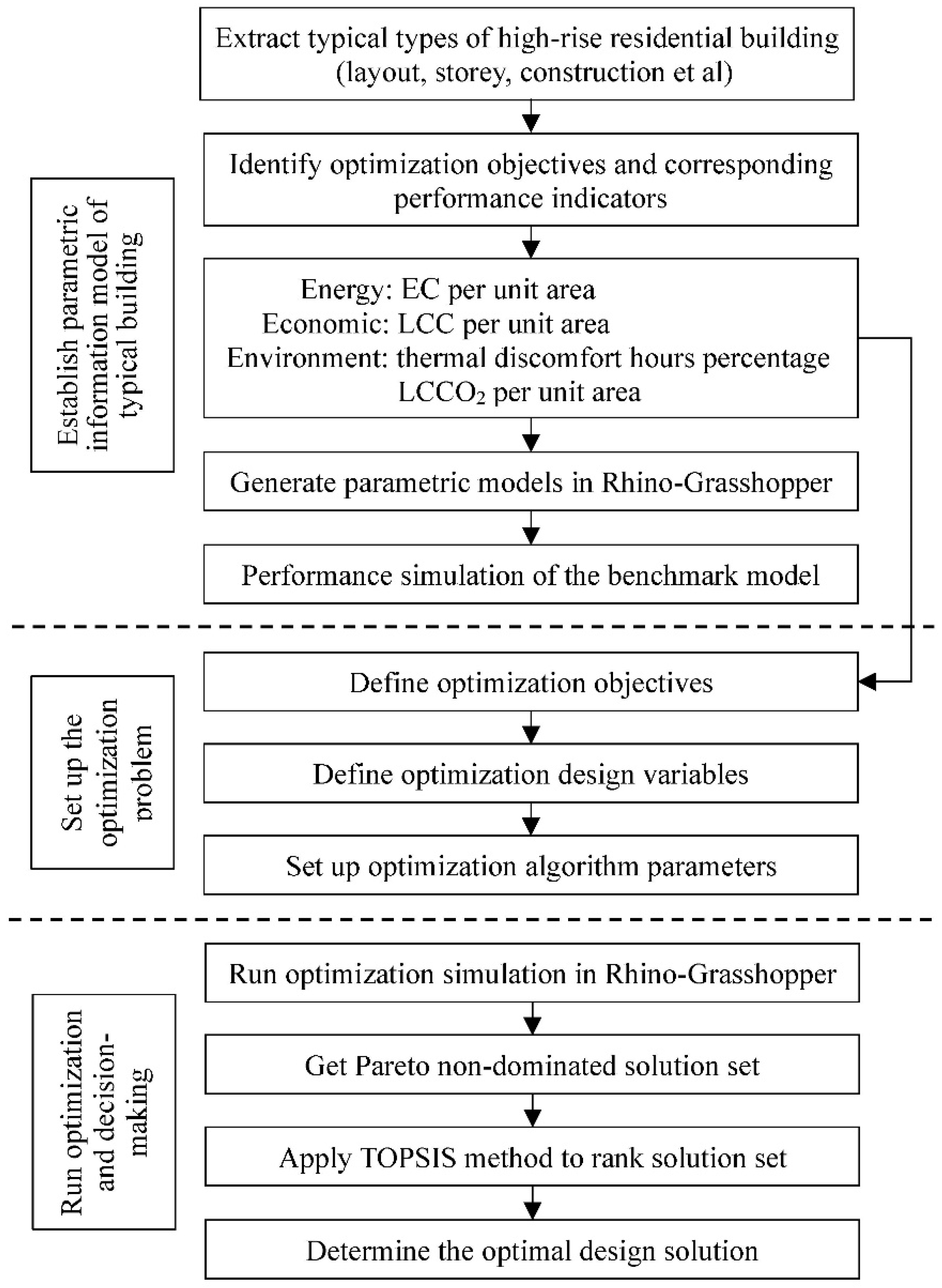
2.1. Optimization Procedure

The flowchart of multi-objective optimization for high-rise residential buildings in this paper is shown in Figure 1; it mainly consists of three steps: first, extract the typical types of high-rise residential buildings by combining survey results with relevant criteria, and establish its parametric performance simulation model in Rhino-Grasshopper according to the determined optimization objectives before simulating the performance of the benchmark building with this model. This step is the foundation of the entire study. Second, set up the simulation-based multi-objective optimization problem, including defining the objective function, optimization variables, and optimization algorithm parameters. Third, run multi-objective optimization to obtain the Pareto non-dominated solution set and analyze the objective function and design variables therein. Meanwhile, apply the TOPSIS method to determine the optimal design scheme.

2.1.1. Building Performance Simulation Tool

The establishment of the residential parametric model and performance simulation was based on the Rhino-Grasshopper visual programming platform. The building energy consumption, thermal environment, and solar radiation simulations were powered by the Honeybee and Ladybug plugins installed in Grasshopper. The Honeybee module can transform the building volume model into a thermal zoning model to form a parametric building hot zone model and directly invoke EnergyPlus (V 9.0) software to complete the simulation of the building’s heating and cooling load and indoor ambient temperature. The simulation results of EnergyPlus were evaluated using the ANSI/ASHRAE standard 140-2007 (ASHRAE 2007) [30]. Many studies have been conducted using EnergyPlus [31,32,33]. Furthermore, in previous studies, the effectiveness of the simulation results was verified using the measured data [34]. The Ladybug module can read and process the climate information file; it has an independent simulation core and can provide various simulations of sunshine and thermal radiation, which can be used to calculate the solar irradiance received by the roof and facade, enabling calculation of the power generation of the solar photovoltaic system.

2.1.2. Multi-Objective Optimization Tool and Algorithm

The multi-objective optimization problem in this study was solved using Octopus, which is another plugin for Rhino-Grasshopper; it can generate the Pareto-optimal solution set by the Strength Pareto Evolutionary Algorithm (SPEA-2) and the Hypervolume Estimation Algorithm (HypE) [35]. Compared with other multi-objective optimization algorithms, SPEA-2 has a greater advantage in the distribution uniformity of solutions derived from environmental selection based on neighbor rules, enabling it to better avoid falling into local optimality [36]. Moreover, SPEA-2 performs better in higher dimensions than NSGA-II [37]. The optimization process was conducted simultaneously with the performance simulation of each generation. All design variables were imported as genes into the Octopus module. The evaluation of four objectives—building energy consumption, thermal comfort, life-cycle cost, and carbon emissions—was attempted. Octopus uses SPEA-2 with hypermutation to automatically control the design variables and constantly search for the minima of the four objectives, thereby providing a solution set, which is a Pareto or non-dominated solution in which there is no other feasible solution that improves one objective without deteriorating at least another one.

2.1.3. Multiple-Attribute Decision-Making–TOPSIS

The output result of a multi-objective optimization model is a Pareto non-dominated solution set composed of a series of optimal solutions; that is, each solution is undifferentiated, making it difficult to judge the advantages and disadvantages of different solutions for the four optimization objectives. A multi-attribute decision-making method is needed to determine the best scheme from a series of design schemes. The Technique for Order of Preference by Similarity to Ideal Solution (TOPSIS) is one of the multi-objective decision-making methods that is used for ranking the alternatives to the decision-making problem; it is based on choosing the alternative that has the closet distance to the ideal positive solution and the longest distance from the ideal negative solution. The ideal positive solution is based on maximizing the beneficial criteria, while the ideal negative solution is based on minimizing the non-beneficial criteria [38,39]. Firstly, the data of the Pareto non-dominated solution set are normalized. Secondly, the weighting method is applied to assign weight coefficients of 0~1 to the four optimization objectives, of which the sum is 1. The weight coefficient reflects the preference of decision-makers, and different decision-makers can change the weight value according to their different needs for the four objectives. Thirdly, the TOPSIS method is used to evaluate the solution set comprehensively in order to judge the closeness between the current optimal solution and the ideal solution. Finally, the optimal scheme is selected according to the degree of proximity. The calculation formulae are as follows:

$$C_i={\displaystyle \frac{D_i}{D_i^{+}+D_i^{-}}}$$

(1)

$$D_i^{+}=\sqrt{{\sum }_{j=1}^m{\omega }_j{\left(Z_j^{+}-z_{ij}\right)}^2}$$

(2)

$$D_i^{-}=\sqrt{{\sum }_{j=1}^m{\omega }_j{\left(Z_j^{-}-z_{ij}\right)}^2}$$

(3)

where C_i is the final score of each evaluation solution, 0 ≤ C_i ≤ 1; when C_i is closer to 1, the evaluation solution is better. $D_i^{+}$ and $D_i^{-}$ are the distances between the ith evaluation object and the optimal scheme or the worst scheme, respectively; $z_{ij}$ is the normalized weighted matrix; $Z_j^{+}$ and $Z_j^{-}$ are the optimal scheme and the worst scheme, respectively, which are composed of the maximum and minimum values of each column element in the matrix; and ω_j is the weight of the jth evaluation index.

2.2. Case Study in Two Cities with Different Solar Radiation

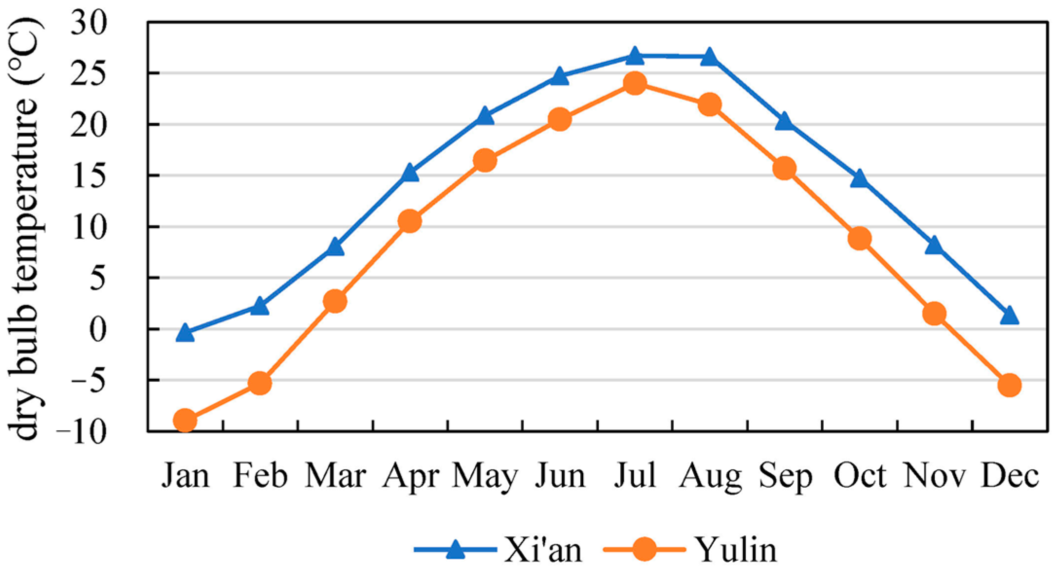
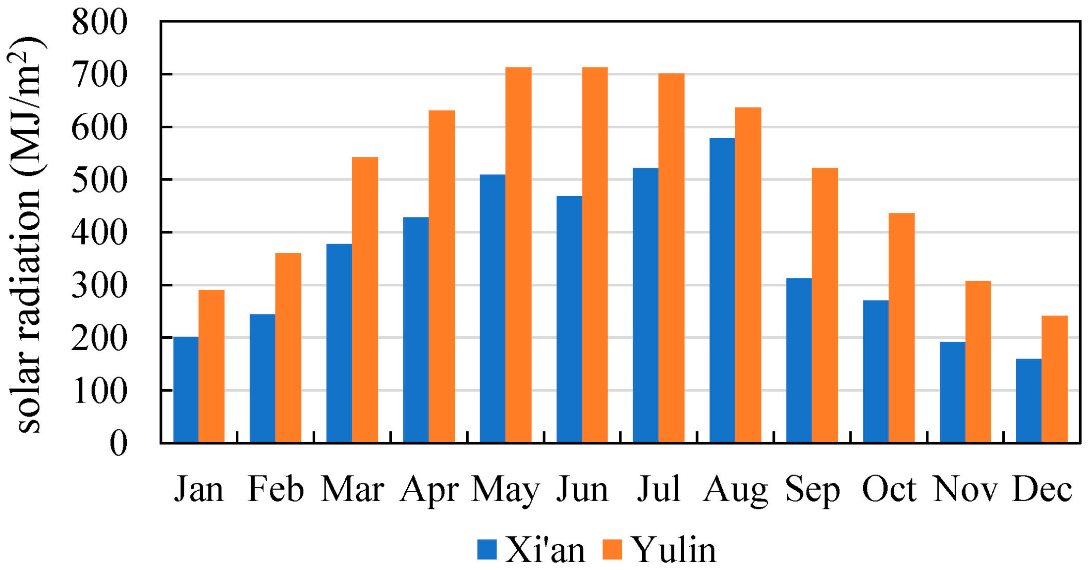
2.2.1. Weather Data

Solar radiation and its utilization will directly affect buildings’ energy consumption, indoor thermal comfort, etc., thereby affecting their carbon emissions and costs during operation, so the optimal design scheme formed under the multi-objective optimization will vary. For the purpose of this study, considering the regionality and design consistency of residential buildings, Xi’an (34°30′ N) and Yulin (38°23′ N), two cities in the same province, were selected for comparative analysis. Moreover, according to the Chinese standard “ GB 50176-2016 Code for thermal design of civil building” [40], both cities are located in cold areas, where the average temperature ranges from −10 °C to 10 °C in the coldest month, and the number of days below the average temperature of 5 °C is between 90 and 145 days.

Figure 2 shows the monthly average dry-bulb temperature, and the annual average temperature is 14.1 °C in Xi’an and 8.5 °C in Yulin, which has a slightly colder climate. However, the cities’ solar energy resources have great differences. As presented in Figure 3, the annual total solar radiation of Xi’an is 4262.1 MJ/m², while Yulin’s is 6093.6 MJ/m² (~43% higher), which may reflect the influence of solar radiation.

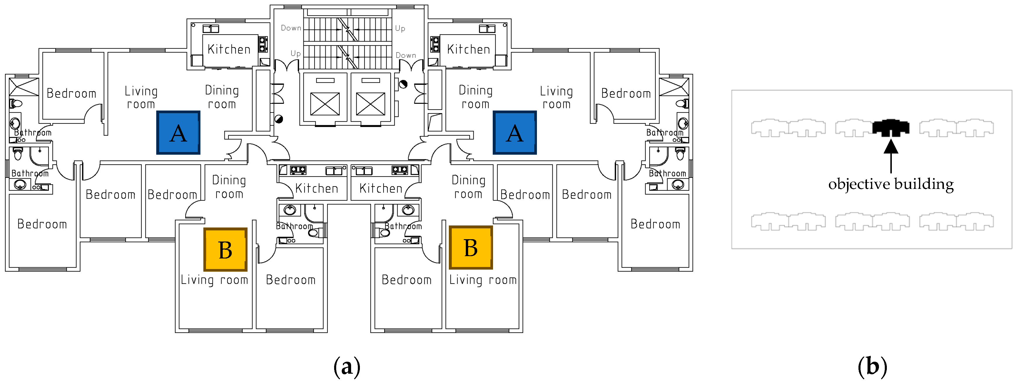
2.2.2. Benchmark Building Specifications

Through the investigation of urban residential buildings in Xi’an and Yulin, a typical building was selected as the carrier for this study. The building faces the south, with 26 stories and a floor height of 3 m and a standard unit composed of four households, including two household types. The building area of A-type households is 115 m², including three bedrooms, a living room, a kitchen, a dining room, and two bathrooms. B-type households, also with an area of 115 m², include two bedrooms, a living room, a kitchen, a dining room, and bathrooms. The south window–wall ratio of one unit is 0.4, while the north window–wall ratio is 0.2. Figure 4a shows the floor plan of a standard unit. Details of the building envelope are provided in

Table 1. Details of the building envelope.

Construction Component	Layers (from Exterior to Interior)	Thickness (mm)	Conductivity (W/m·K)	Density (kg/m3)	Specific Heat (J/kg·K)
Roof	40 mm fine aggregate concrete	40	1.74	2500	920
	XPS	——	0.03	35	1647
	3 m SBS waterproof layer	3	0.23	900	1680
	20 mm cement mortar	20	0.93	1800	1050
	120 mm reinforced concrete	120	1.74	2500	920
	20 mm mixed mortar	20	0.87	1700	1050
Exterior wall	20 mm cement mortar	20	0.93	1800	1050
	XPS	——	0.03	35	1647
	20 mm cement mortar	20	0.93	1800	1050
	200 mm aerated concrete	200	0.22	700	1050
	20 mm mixed mortar	20	0.87	1700	1050
Exterior window	Clear glass	6	0.76	1800	1260
	Air cavity	6	0.026	1.293	1005
	Clear glass	6	0.76	1800	1260

Note: The thickness of XPS is an optimization variable in the following text.

. The building energy consumption and indoor thermal comfort index of this building with no insulation layer, sunvisor, or solar energy utilization were taken as the benchmark for comparison. Considering the influence of building orientation and occlusion on the amount of solar radiation received by the building facade, according to the local residential sunshine hours [41] and fire spacing requirements, the north–south spacing of the residential building was set at 72 m, while the east–west spacing was 13 m. A unit of the middle building was selected as the research object, as shown in Figure 4b.

2.2.3. Objective Functions

Based on a comprehensive consideration of energy, economy, and the environment, the optimization objectives were set as follows: building energy consumption (EC), life-cycle cost (LCC), thermal discomfort hours percentage (TDHP), and life-cycle carbon emissions (LCCO₂).

Building Energy Consumption

Building energy consumption generally includes heating, cooling, lighting, and equipment energy use. This paper mainly reduces energy consumption from the perspective of passive design, and the design variables do not involve the parameters related to equipment; therefore, the energy consumption for hot water, electrical appliances, and lighting is the same for each scheme and is not affected by design variables, so the heating and cooling energy consumption is mainly calculated during the optimization process. Through the Rhino-Grasshopper platform, we used the Honeybee plugin to invoke the EnergyPlus engine to simulate energy consumption. Chinese Standard Weather Data (CSWD) for Xi’an and Yulin were used for meteorological parameters. The heating period was set as 15 November to 15 March, with the indoor temperature calculated at 18 °C and the air change rate calculated at 0.5 h⁻¹. The cooling period was set as 15 June to 31 August, with the indoor temperature calculated at 26 °C and the air change rate calculated at 1.0 h⁻¹. There is no heating or cooling equipment in the bathroom or kitchen. For other spaces, in order to increase the simulation speed while reducing the impact of simplification [42], the building was divided into two thermal zones: the bedroom, and the living and dining rooms. The personnel occupancy rate, heating and cooling equipment control mode, and time in each thermal zone were set uniformly according to Appendix C of the “JGJ/T 449-2018 Standard for green performance calculation of civil buildings” [43].

Life-Cycle Cost

Life-cycle cost is an important index to measure the economy of design schemes, including the costs of investment, operation, replacement, and maintenance. A 30-year period was considered for the life-cycle analysis. The lifespans of insulation materials, windows, and shading devices are generally 30 years or longer; therefore, their replacement costs are not taken into account [22]. Life-cycle analysis mainly considers the present value of the investment and operating costs. As for the investment cost, since the main structure and the cost of labor and transportation of different design schemes are essentially the same, the initial investment cost does not need to calculate the absolute value but only the incremental cost generated by the change in the optimization design variable. On the basis of the standard BS EN 15459-1 [44], the value can be calculated using Formula (4):

LCC = dIC + PWF·ECC

(4)

where dIC is the difference in investment cost between the optimization scheme and benchmark building (CNY/m²), PWF is the present worth factor in the life cycle, and ECC is the annual building energy consumption cost (CNY/m²); the CNY–USD (EUR) exchange rate is ~0.137 (0.126).

ECC includes the corresponding cost of energy consumption for heating and cooling, calculated as shown in Formula (5):

ECC = Q_H·P_H/H·η_H + (Q_C/η_C − E_PV)·P_E

(5)

where Q_H is the annual heating load (kW·h/m²), P_H is the price of coal (750 CNY/ton), H is the electric conversion coefficient of coal (8.14 kW·h/kg), η_H is the efficiency of the heating system (0.81; pipe network efficiency of 0.92 and boiler efficiency of 0.88), Q_C is the annual cooling load (kW·h/m²), η_C is the efficiency of the cooling system (3.0), E_PV is the annual power generation of the photovoltaic system (kW·h/m²), and P_E is the electricity price (0.49 CNY/kW·h).

PWF is used to convert the future value of funds to the present value, and the calculation method is expressed in Formulae (6)–(8) [45]:

PWF = (1 − (1 + r_e)⁻ⁿ)/r_e

(6)

r_e = (r − e)/(1 + e)

(7)

r = (r_i − f)/(1 + f)

(8)

where r_e represents the market rates that take into account the rising value of energy (%), r is the actual rate (%), e is the rate of increase in energy prices (1.2%), n is the life-cycle span (30 years), r_i is the nominal interest rate (7%), and f is the inflation rate (2%).

Thermal Discomfort Hours Percentage

Taking optimization measures to reduce buildings’ energy consumption may have a negative impact on the indoor thermal environment. Therefore, the percentage of annual thermal discomfort hours in a full year (i.e., 8760 h) is used as an indoor thermal environment evaluation index. Although the relevant standards specify the indoor calculated temperature in winter and summer, this is mainly used to calculate the heating and cooling energy consumption, and it is not equal to the actual indoor temperature. Considering the thermal adaptability and self-regulation ability of the human body, with reference to relevant studies [46], indoor comfort is determined when the air temperature is at 1~28 °C, and its value can be directly output by EnergyPlus (V 9.0) software. TDHP can be calculated as shown in Formula (9):

$$\mathrm{T}\mathrm{D}\mathrm{H}\mathrm{P}={\displaystyle \frac{1}{8760·n}}{\sum }_{i=1}^n{TDH}_i$$

(9)

where TDHP is the average value of the annual cumulative thermal discomfort hours percentage for each thermal zone (%), ${TDH}_i$ is the annual thermal discomfort hours for each thermal zone (h), and n is the number of thermal zones.

Life-Cycle Carbon Emissions

The carbon emission factor (CEF) method is used to calculate buildings’ carbon emissions. The CEF is a coefficient that represents the quantity of CO₂ and its equivalents emitted from one unit of a certain type of material or fuel. Corresponding to the calculation of life-cycle cost, the calculation of life-cycle carbon emissions includes the carbon emissions of building materials used in optimization design and the building’s operating phase, as well as taking into account the carbon reduction provided by solar photovoltaic output. The calculation method is shown in Formula (10):

$${\mathrm{LCCO}}_2={\sum }_{i=1}^n{M}_i·F_i/A+n·[Q_H·E{F}_{standard coal}/H·{\eta }_H+(Q_C/{\eta }_C-E_{PV})·E{F}_{electricity}]$$

(10)

where $M_i$ is the consumption of material of type i, $F_i$ is the CEF of material of type i, (kgCO₂/unit material quantity; see Appendix D of “GB/T 51366-2019 standard for building carbon emission calculation” [47]), A is the building area (m²), EF_{standard coal} is the CEF of standard coal (according to Appendix A of GB/T 51366-2019, the value is 0.094 KgCO₂/MJ = 2.77 KgCO₂/Kg), and EF_electricity is the CEF of electricity (in line with the “2019 Annual Emission Reduction Project China Regional Power Grid Baseline Carbon Emission Factors”, the value is 0.8922 kgCO₂/kWh). The meanings of the other parameters are the same as those in the Section Life-Cycle Cost.

Photovoltaic Power Generation Estimation

In order to make full use of solar radiation resources, it is assumed that solar photovoltaic panels are installed on the roof and south exterior wall of high-rise residential buildings. Considering the full use of solar radiation, the photovoltaic panels on the roof are laid at an angle of 30° and installed vertically on the south wall, except for the window areas.

According to the provisions of “GB/T 51366-2019 standard for building carbon emission calculation” [47], the annual power generation of the photovoltaic system can be estimated according to Formula (11):

E_PV = I·K_E (1 − K_S)·A_P

(11)

where E_PV is the annual power generation of the photovoltaic system (kW·h), I is the annual solar irradiance of the photovoltaic panel surface obtained via Ladybug dynamic simulation (kW·h/m²), K_E is the conversion efficiency of the photovoltaic cells (set at 15% for monocrystalline silicon photovoltaic cells), K_S is the loss efficiency of the photovoltaic system (set at 25% in line with the above criteria), and A_P is the photovoltaic panels’ net area of the photovoltaic system (m²).

2.2.4. Design Variables

The principle of design variable selection mainly includes two aspects: one is to reflect the passive design and the other is to be related to the four objectives. From this point, according to the theoretical calculation method of building energy consumption, the influencing factors mainly include the building’s shape, orientation, interface, and envelope construction. Building shape mainly reflects the length, width, and height of a building, but the building’s performance is optimized under the premise of meeting the reasonable use function in this paper, i.e., a certain plane and layout, so we did not take this as a variable. In relation to the objective function, building orientation has a direct impact on the indoor thermal environment and energy consumption, which, in turn, affect the cost and carbon emissions in the operating phase. The building interface includes the window–wall area ratio, sunshade, etc., while the envelope construction includes the exterior wall, roof, window types, etc. These variables all directly affect the four optimization objectives.

Some specific instructions are as follows: The east and west exterior walls of high-rise residential buildings usually do not have windows or they have small windows. In the benchmark model established in this paper, the east and west exterior walls are only equipped with external windows that meet the ventilation requirements of the bathroom, so they were taken as fixed values during optimization, and only the south and north window–wall ratios were taken as optimization variables. Correspondingly, the south and north exterior window types were also used as optimization variables, and 3 types of exterior windows were set. As the main structure of the exterior wall and roof was unchanged, their thermal performance was mainly affected by the thickness of the insulation layer, so the insulation layer thickness of the exterior wall and roof was taken as the optimization variable. Considering the differences in solar radiation effect in various orientations, the insulation layer thickness of different oriented external walls was also taken as an optimization variable. Taking into account the demand of summer heat protection for residential buildings, a horizontal sunvisor is set in the south exterior window, and the overhang length was taken as an optimization variable. Finally, eleven design variables were determined for optimization. Referring to the survey results and relevant standards, we considered the value extensibility of the design variables. The value ranges of the design variables, material selection, and price were determined.

Table 2. Optimized design variables and parameter settings.

Number	Design Variable	Symbol	Type	Range	Step
1	Building orientation (°)	O	Continuous	−45°~45°	5°
2	South window–wall ratio	Swwr	Continuous	0.3~0.6	0.05
3	North window–wall ratio	Nwwr	Continuous	0.15~0.3	0.05
4	South exterior window type	Swin	Discrete	3 Types	——
5	North exterior window type	Nwin	Discrete	3 Types	——
6	Insulation layer thickness of the south wall (m)	St	Continuous	0~0.2	0.01
7	Insulation layer thickness of the north wall (m)	Nt	Continuous	0~0.2	0.01
8	Insulation layer thickness of the east wall (m)	Et	Continuous	0~0.2	0.01
9	Insulation layer thickness of the west wall (m)	Wt	Continuous	0~0.2	0.01
10	Insulation layer thickness of the roof (m)	Rt	Continuous	0~0.2	0.01
11	South horizontal sunvisor overhang length (m)	L	Continuous	0~1.0	0.1

shows the name, symbol, type, range, and step of each variable. The materials, prices, and carbon emission factors of the insulation layer, exterior windows, sunvisor, and photovoltaic panels are displayed in

Table 3. Price and carbon emission factor (CEF) for different kinds of materials.

Number	Name	Material		Price	CEF
1	Insulation layer	XPS board		850 CNY/m3	175.7 kgCO2/m3
2	Exterior window	A: 6 mm Low-E + 9A + 6 mm clear	K = 1.977 W/m2·K SHGC = 0.568 Tvis = 0.745	680 CNY/m2	134 kgCO2/m2
		B: 6 mm Low-E + 9A + 6 mm Low-E	K = 1.513 W/m2·K SHGC = 0.477 Tvis = 0.709	870 CNY/m2	147 kgCO2/m2
		C: 6 mm Low-E + 9A + 6 mm clear + 9A + 6 mm Low-E	K = 1.182 W/m2·K SHGC = 0.436 Tvis = 0.631	1050 CNY/m2	164 kgCO2/m2
3	Sunvisor	60 mm concrete slab		120 CNY/m2	17.7 kgCO2/m2
4	Photovoltaic panel	Monocrystalline silicon solar panel		640 CNY/m2 (4 CNY/W)	30 kgCO2/m2

.

2.2.5. Algorithm Parameter Settings

The optimization problem in this research is a four-objective optimization problem, and the Pareto front was used to find the trade-off solutions. We set the optimization parameters in the Octopus plugin of Grasshopper. Elitism gives the percentage of new solutions that are bred out of the elite instead of the entire pool. When set high, more local optimization is performed. Mutation probability is the probability of each parameter/gene becoming mutated with the mutation rate. A low mutation rate means few changes to the parameters’ values, while a high rate means significant changes. The crossover rate is the probability of two subsequently generated solutions exchanging parameter values. Referring to relevant studies [22,48] and the Octopus module, the elitism, mutation probability, mutation rate, and crossover rate were 0.5, 0.2, 0.9, and 0.8, respectively. The population size was set to 60, which is more than five times the number of variables, and the optimization process would terminate after 25 generations, i.e., the maximum number of iterations was 1500.

3. Results and Discussion

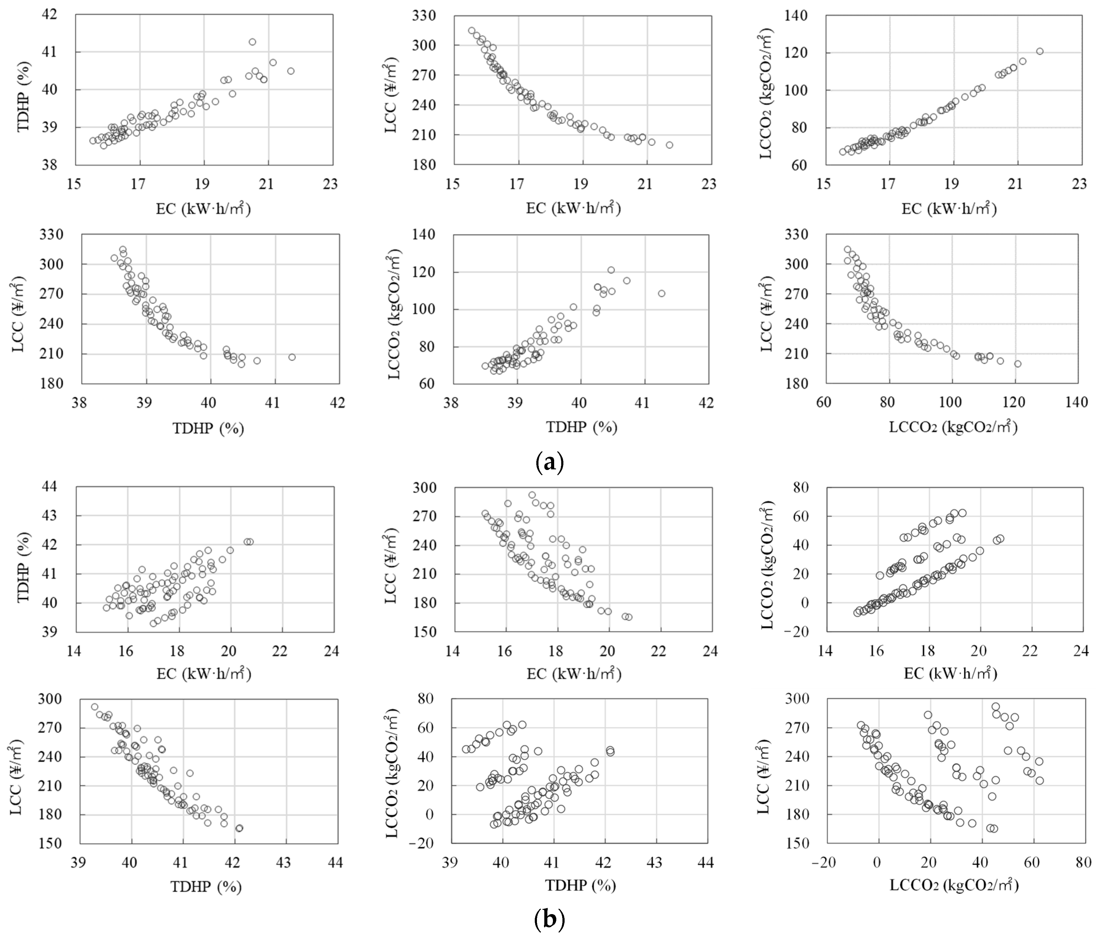
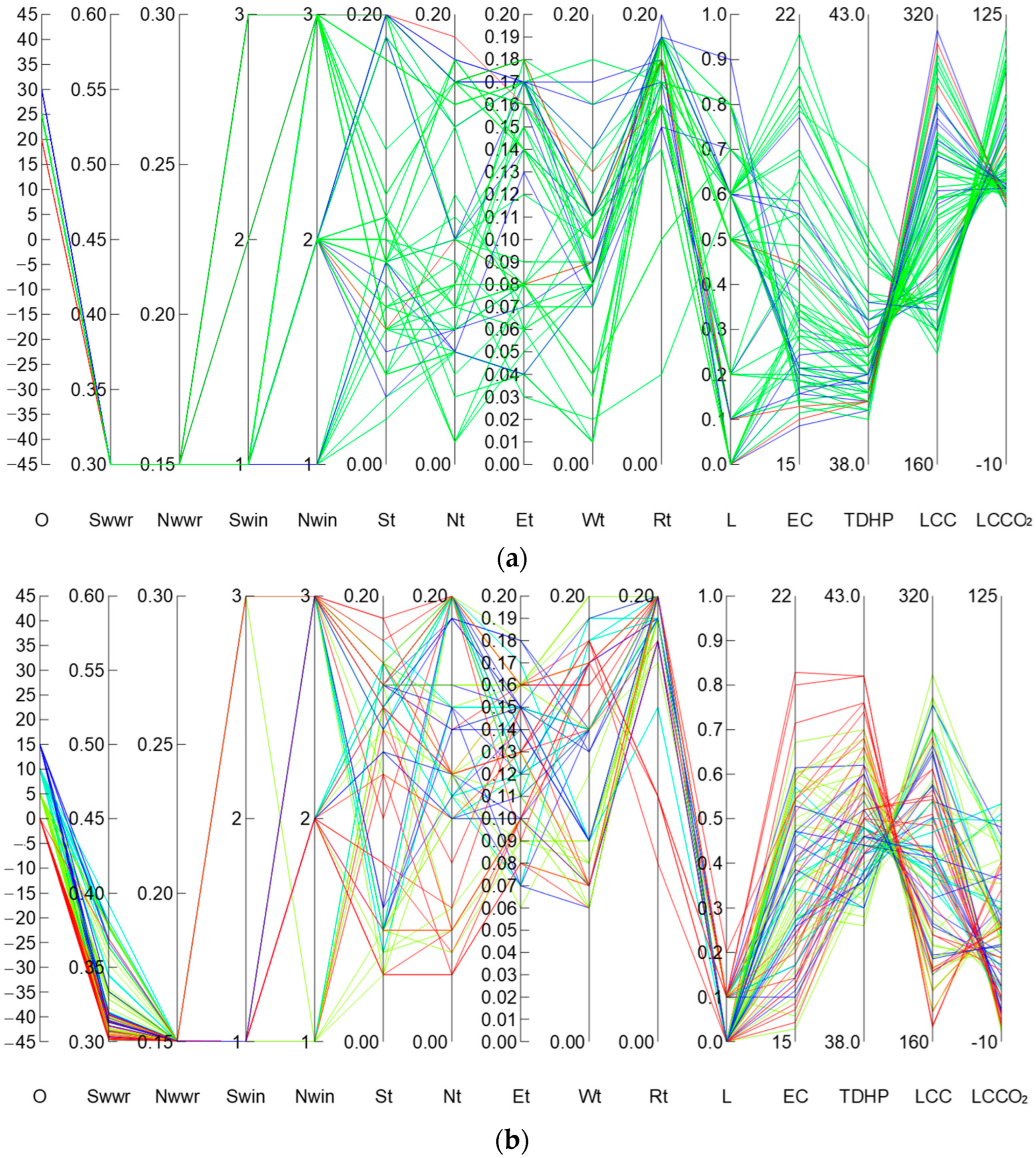
3.1. Tradeoffs of Multi-Objective Optimization and Its Value Distribution

Non-dominated values of objectives in the form of Pareto fronts were returned after 25 generations of calculation. There were 65 and 82 non-dominated solutions for Xi’an and Yulin, respectively. The 4D Pareto front was mapped to a bidimensional (2D) graph, and the relationships between the bi-objective Pareto solutions for Xi’an and Yulin are displayed in Figure 5.

For the trade-off relationships between the multiple objectives, as shown in Figure 5, in Xi’an, there are incomplete positive correlations between EC and TDHP, EC and LCCO₂, and LCCO₂ and TDHP, while there are nonlinear incomplete negative correlations between EC and LCC, LCC and TDHP, and LCC and LCCO₂. It can be seen that although the correlation is positive, due to the guidance of the four objectives, the pairwise correlation can only reflect the incomplete correlation, and there is a contradictory relationship among the objectives. For Yulin, there is a similar correlation but greater dispersion. The relationship between two objectives consists of multiple parallel curves. For example, when the building energy consumption is the same, there exist several values of TDHP, LCC, and LCCO₂, with large differences. This happens because the objective function considers the offsetting effect of solar power generation, and the solar radiation in the Yulin area is stronger. Under the influence of this factor, the design variables and objective functions form the distribution characteristics of solution sets different from those in the Xi’an area. The details of the relationships between the objectives and variables will be explained in Section 3.2.

In terms of the value distribution of objective functions, as can be seen in Figure 5a, the EC of the Pareto solution set is distributed at 15.6~21.7 kW·h/m² in the Xi’an area; that is, when the designer selects the non-dominated solution, the maximum difference is 6.1 KWh/m². The variation range of TDHP is 38.5%~41.3%, with a maximum difference value of 2.8%. The LCC ranges from 199.3 to 314.4 CNY/m², with a gap of 115.1 CNY/m² between the optimal and the worst solution, while the span for the LCCO₂ is 66.8~120.8 kgCO₂/m², with a maximum difference of 54.0 kgCO₂/m². Regarding the Yulin area, as shown in Figure 5b, the EC ranges from 15.2 kW·h/m² to 20.8 kW·h/m², and there exists a gap of 5.7 kW·h/m² between the maximum and minimum values. The TDHP variation ranges from 39.3% to 42.1%, with a maximum difference value of 2.8%. The LCC is distributed at 161.7~291.8 CNY/m², with a maximum difference of 130.1 CNY/m², while the range for the LCCO₂ is −7.0~62.2 kgCO₂/m², with a gap of 69.2 kgCO₂/m². From the statistical results, the distribution range of LCC and LCCO₂ in Yulin is wider, and the carbon emissions also appear negative because of the carbon reduction effect of photovoltaic power generation. However, the distribution of EC and TDHP shows little difference from that in Xi’an.

In terms of the sensitivity of objectives to the scheme, the response degree of the Pareto solutions to the four objectives is different. LCC has the largest numerical distribution interval, followed by LCCO₂ and EC, while TDHP has the smallest distribution span. This indicates that the adjustment of the design variables has a significant impact on the first three objective functions, while the effect on TDHP is relatively small. Focusing on the influence of each objective on the comprehensive evaluation for design schemes, entropy values were applied to judge the dispersion degree of each indicator. The smaller the information entropy value, the greater the dispersion degree of the indicator, indicating a greater influence of the indicator on the comprehensive evaluation. The orders of the four objectives were calculated for the two cities as follows: for Xi’an, LCC > EC ≈ LCCO₂ > TDHP; for Yulin, LCC > LCCO₂ > EC = TDHP. This shows that the influence of each objective on the comprehensive evaluation also varies in different regions.

3.2. Distribution Characteristics of Design Variables and Their Formation Causes

Based on the Pareto non-dominated solution set obtained via multi-objective optimization, SPSS (V 20.0) software was used to analyze the distribution frequency of eleven design variables and explore their interaction mechanisms with the objective functions to explain their formation causes in different regions.

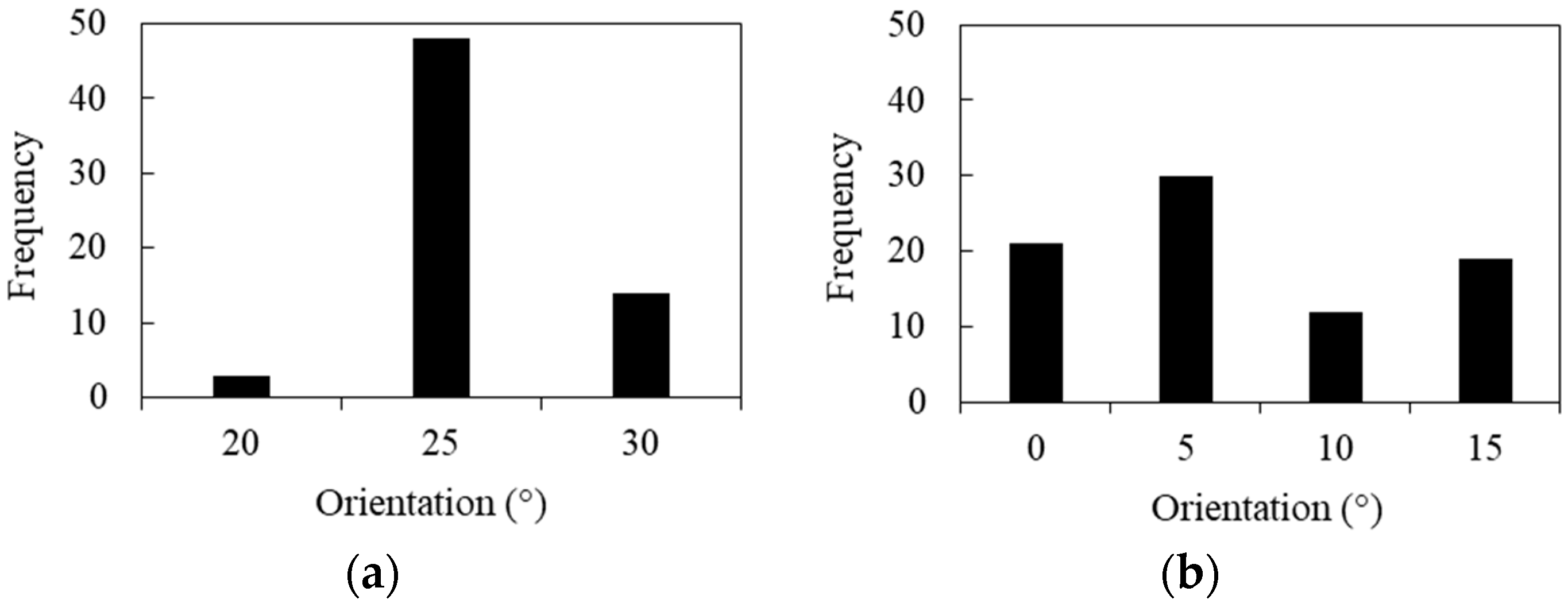
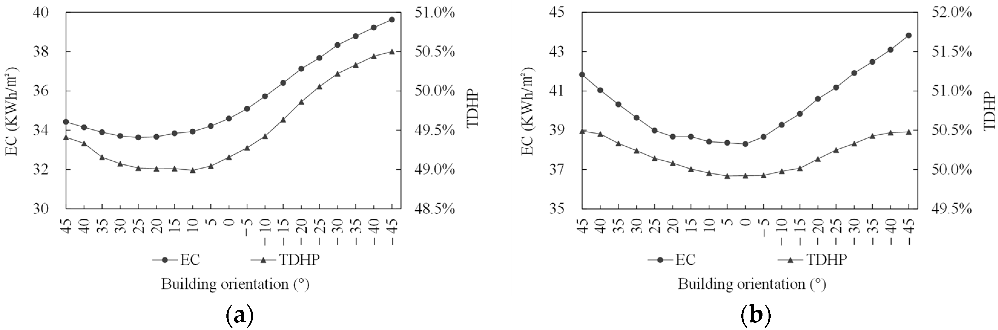
3.2.1. Effect of Building Orientation

As can be seen from Figure 6, in the Pareto solutions, the building orientation distribution is concentrated in the range of 20°~40° south by west for Xi’an; the corresponding value is 0°~15° south by west in Yulin. The difference in building orientation distribution between the two regions is mainly affected by climatic conditions such as solar radiation. Figure 7 presents the relationship of building orientation with EC and TDHP. It can be seen that with the rotation of the building orientation from south by west (45°) to south by east (−45°) in the two regions, the EC and TDHP have the same change rule, both showing a trend of first decreasing and then increasing, but the orientation range corresponding to the low-value interval is different. Meanwhile, the values of building orientation in the Pareto solution set concentration all fall in the trough of the EC and TDHP curve—that is, consistent with the low-value interval. Due to the interaction between the building orientation and other design variables, the best orientation is not unique, and the frequency of each orientation is different. This allows for greater flexibility in the choice of orientation, especially when there are environmental constraints, rather than relying solely on the minimum value of a certain objective.

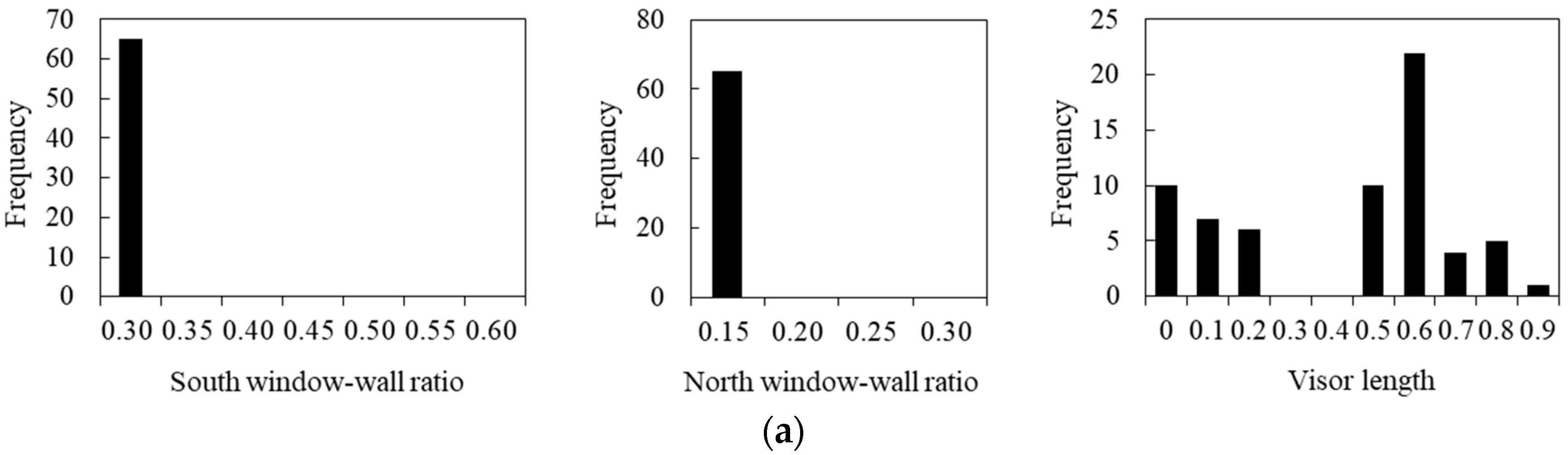
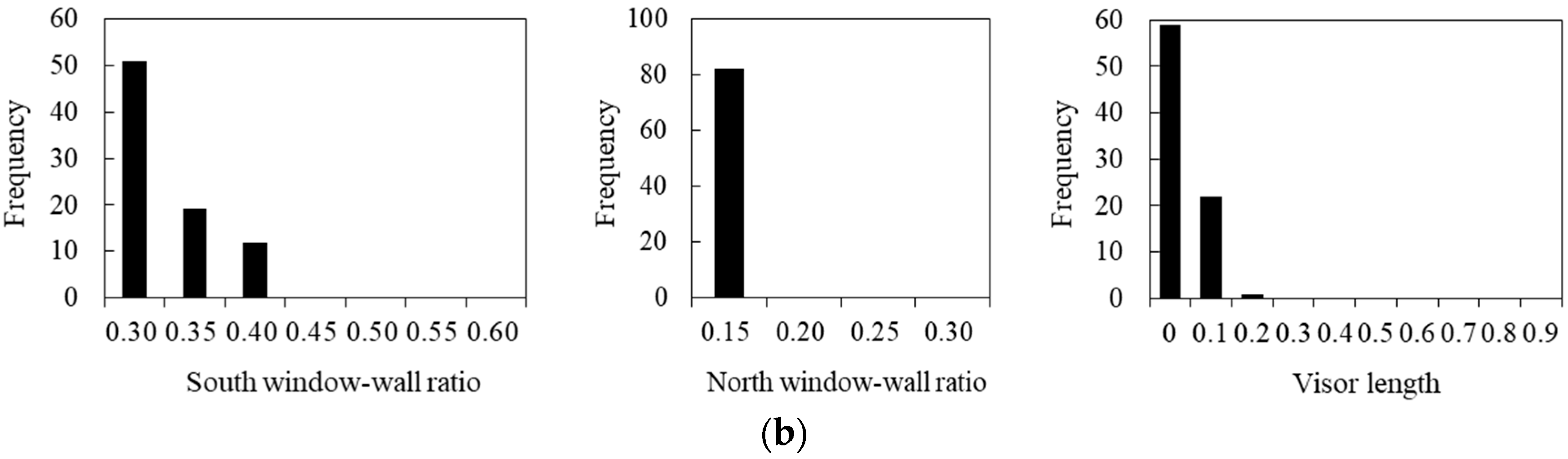
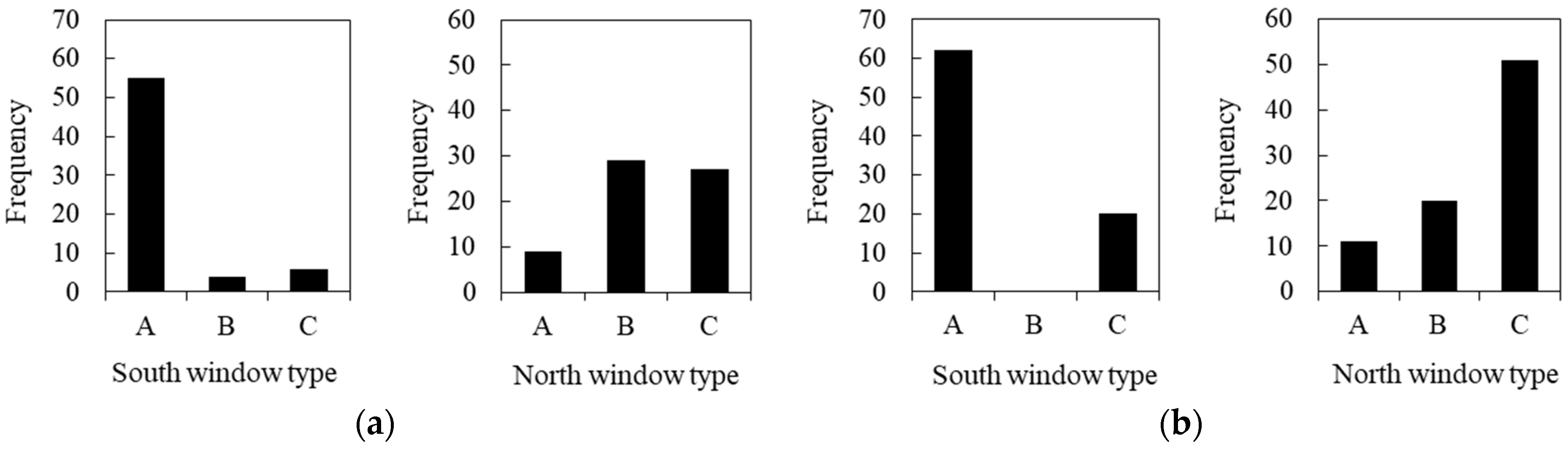
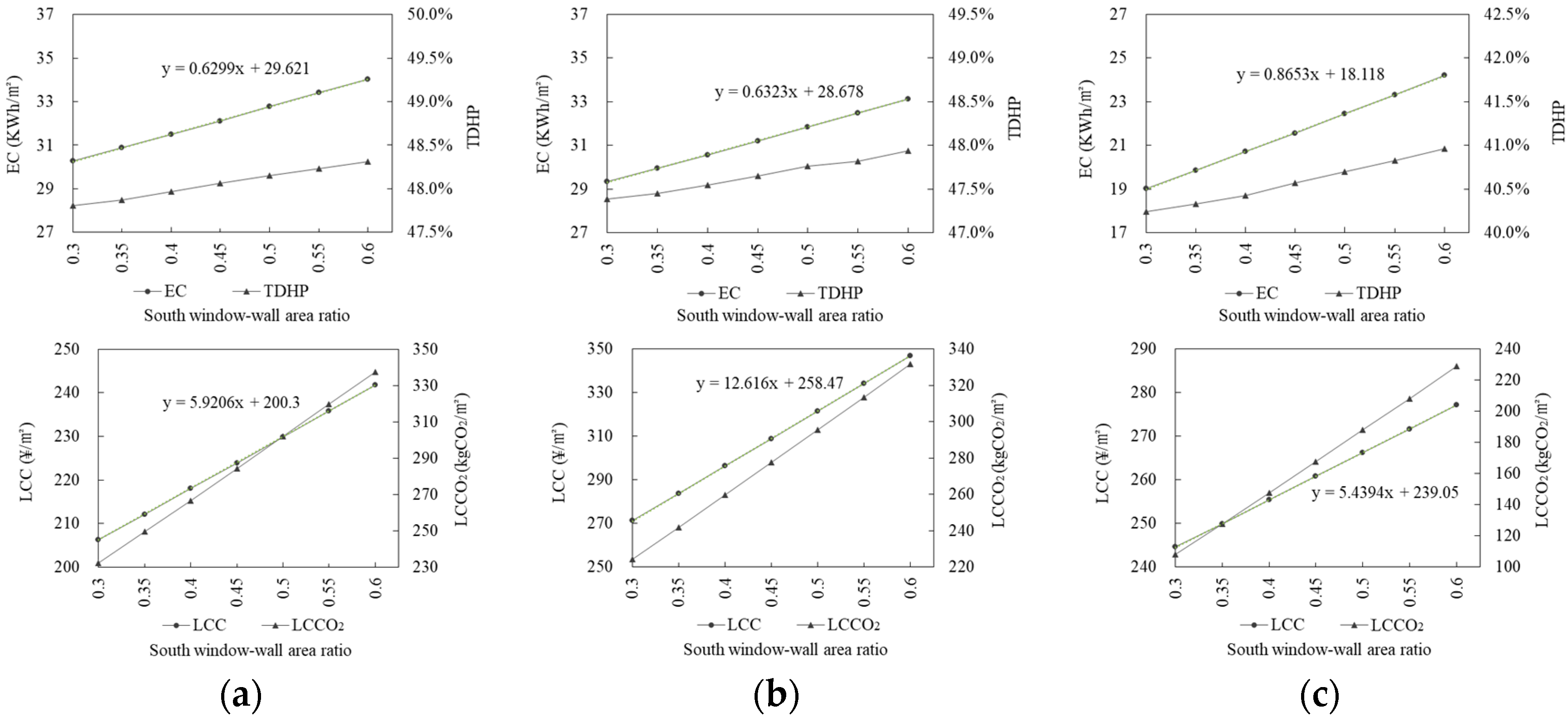
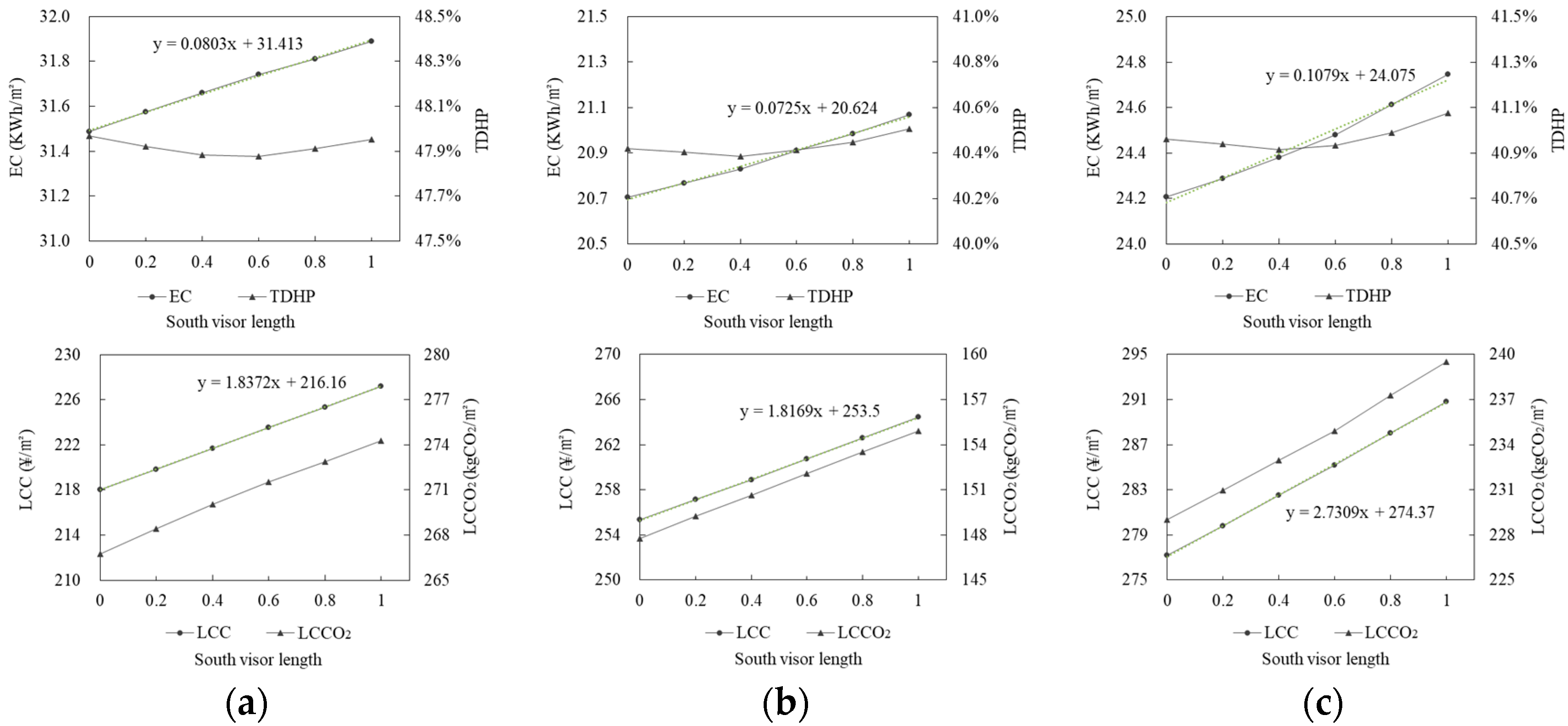
3.2.2. Effect of Window–Wall Ratio, South Sunvisor Overhang Length, and External Window Type

The statistical results for the window–wall ratio, south sunvisor overhang length, and external window type in the Pareto non-dominated solution set are shown in Figure 8 and Figure 9. For the north window–wall ratio, the values in Xi’an and Yulin are the same, at 0.15 (i.e., the lower limit of the given window–wall ratio range). Although there is a large difference in solar radiation between the two regions, the impact on the building’s north side is small, and the smaller the window–wall ratio, the more conducive to reducing the building energy consumption, cost, and carbon emissions of the external windows. This indicates that the lower limit of the given interval can be directly chosen for the north window–wall ratio design. As for the south window–wall ratio, there exists some difference between the two regions. The values of Xi’an are all at the lower limit of the given interval, i.e., 0.3, while the value of 0.3 occupies the largest proportion in Yulin, but 0.35 and 0.4 are also distributed. The south sunvisor’s overhang length in the Yulin area is mainly 0~0.1 m. Mainly due to the colder climate, the heating energy consumption accounts for a relatively high proportion of EC, while the cooling energy consumption is very small, so a smaller sunvisor is more conducive to reducing EC while also decreasing the LCC and LCCO₂. The overhang length in Xi’an ranges from 0 to 0.2 m and from 0.5 to 0.9 m, distributed at both ends, which is mainly formed by multi-objective control. The reasons behind the values of these two variables will be further analyzed in the following text, along with the influence of single factors on objective functions.

For the window type, although external windows with better thermal performance are beneficial for reducing energy consumption and improving the indoor thermal environment, the investment cost and production carbon emissions are higher. In the Xi’an area, the south window types are mainly distributed in type A. The winter climate in Yulin is colder, and the proportion of type-C windows increases, but the solar radiation in this area is stronger, and the solar heat gain coefficient of type A is higher, which is more beneficial for the introduction of solar radiation, so the proportion of this type is still high. With respect to the north window, all three types were selected in both regions, and the proportion of type C in Yulin was higher than that in Xi’an.

Considering the interaction between the window–wall ratio and thermal performance of the building envelope, three cases were set to analyze the effects of the south window–wall ratio on the objective functions based on the benchmark building, as follows: ① the external window is type A; ② the external window is type C; ③ the insulation layer thickness of the roof and external wall is set as 0.1 m, and the external window is type A. Figure 10 presents the relationship between the south window–wall ratio and the four objectives in Xi’an. With an increase in the south window–wall ratio, the values of the four objectives all show an increasing trend, but the degree of influence on each objective is different. Compared with case-1, the change in the window–wall ratio increases the variation amplitude of the four objectives in case-2, while for case-3, the changes in EC, TDHP, and LCCO₂ increased, and the change in LCC decreased. In general, the influence of the south window–wall ratio on the four optimization objectives in the Xi’an area is in the same direction, and the larger the window–wall ratio, the more unfavorable, so its value is the lower limit of the given range.

Figure 11 shows the relationship between the south window–wall ratio and the four objectives in Yulin. Compared with Xi’an, the influence rule demonstrated in Yulin is different. With the increase in the south window–wall ratio, the EC, LCC, and LCCO₂ showed an increasing trend, while TDHP decreased, affecting each objective in a different direction. There was a single linear relationship between the window–wall ratio and each objective, and the change rate of EC, LCC, and LCCO₂ was higher than that of TDHP, so the value range extended to 0.4 after optimization and tradeoff, forming a solution set distribution different from that of Xi’an. Similarly, compared to case-1, the variation amplitude of the four objectives increased in case-2; for case-3, the variation range of EC, TDHP, and LCCO₂ increased, while that of LCC decreased. Comparing the two regions, the influence amplitude of the window–wall ratio on EC was essentially the same under the same conditions, and the effect was in the same direction, while the TDHP was also similar, but the effect was in the opposite direction. The effects on LCC and LCCO₂ were quite different, and the window–wall ratio of residential buildings in Yulin had a greater impact on these two objectives.

For the sunvisor, the optimization results show that it is not appropriate or that only a small sunvisor should be used in Yulin, so the influence of sunvisor overhang length on the four objectives was analyzed only for Xi’an. Moreover, considering the interaction of the design variables, three cases were set, as follows: ① based on the benchmark building, a type A window is adopted; ② on the basis of case-1, the roof and external wall are provided with a 0.1 m thick insulation layer; ③ on the basis of case-2, the window–wall ratio is set to 0.6. As shown in Figure 12, with the increase in sunvisor overhang length, the EC, LCC, and LCCO₂ increased linearly, while the TDHP first decreased and then increased. Comparing case-2 to case-1, the variation amplitude of the four objectives was slightly reduced, indicating that the influence of the change in sunvisor length on each objective was weakened after the thermal performance of the building envelope was improved. Comparing case-3 and case-2, the variation amplitude of the four targets increased significantly, revealing that the change in sunvisor length enhances the influence on each objective when the south window–wall ratio is increased. Therefore, given the different direction and amplitude of the effect of overhang length on each objective, the value distribution formed by the balance of the multiple objectives is displayed in Figure 8a, where the median value (0.3~0.4 m) and upper limit value (1.0 m) of the variable range are not filtered as the parameter values of the Pareto solution set.

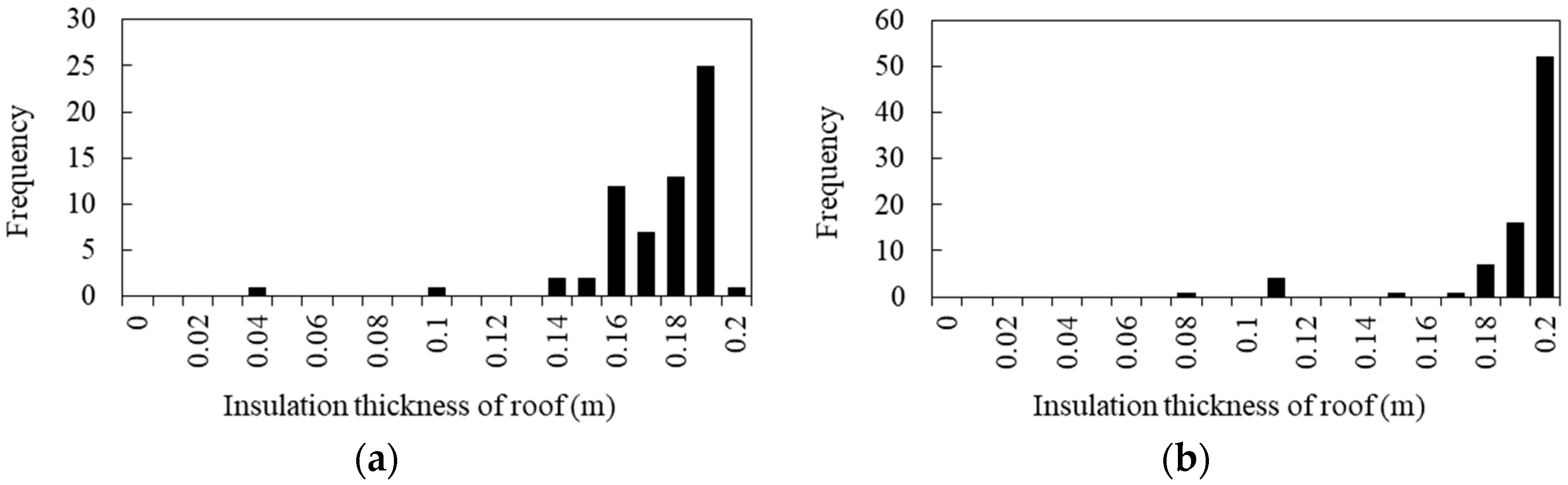
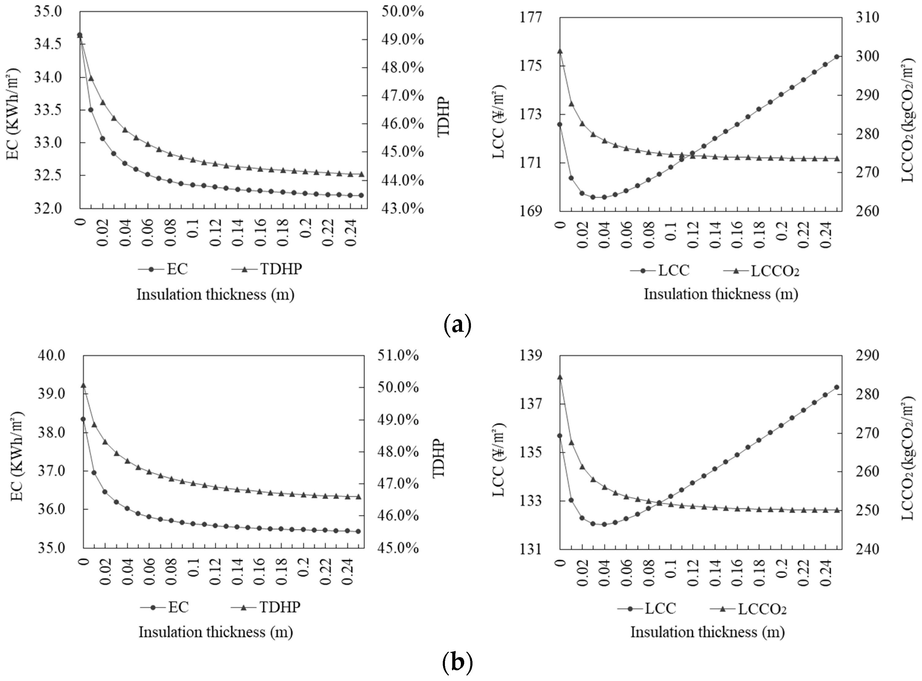
3.2.3. Effect of the Roof’s Insulation Layer Thickness

Figure 13 shows the value distribution of the roof insulation layer thickness in Pareto solutions. In the Xi’an area, the insulation layer thickness is mainly concentrated above 0.14 m, and the range of 0.16~0.19 m occupies the largest proportion (~88%). The value distribution in Yulin is more concentrated, mainly above 0.18 m, of which 0.2 m accounts for up to 64%. The mean thickness of the insulation layer in Yulin is 0.19 m, which is higher than that in Xi’an (0.17 m), revealing that the thickness of the roof insulation layer is more inclined to the upper limit area of the given interval.

Based on the benchmark model, the relationship between roof insulation layer thickness and the four objectives is demonstrated in Figure 14. As shown, the change rule of the two regions is effectively the same; with the increase in insulation layer thickness, EC, TDHP, and LCCO₂ show a trend of obviously reducing at first, followed by a slow decrease; LCC displays a trend of first decreasing and then increasing, and the insulation layer thickness corresponding to the inflection point is ~0.04 m. In terms of objective values, under the influence of climatic conditions and solar radiation, the EC and TDHP of Xi’an are lower than those of Yulin with the same insulation layer thickness, but Xi’an’s LCC and LCCO₂ are higher. This shows that the use of solar radiation can reduce the life-cycle cost and carbon emissions. The influence of the insulation layer thickness on the four objectives is contradictory, with different effect amplitudes, as well as being subject to the other design variables interacting to form the value distribution shown in Figure 13.

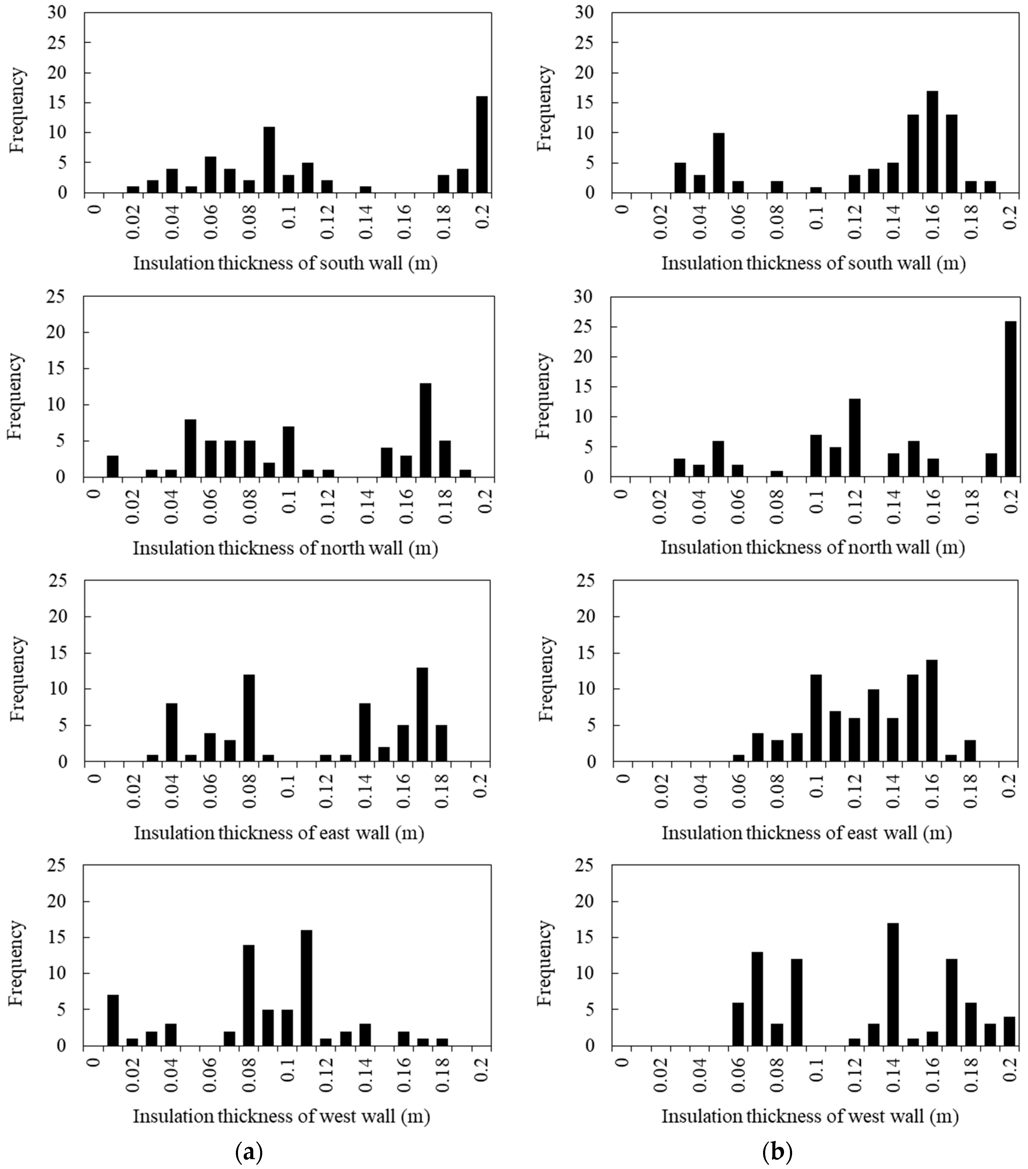
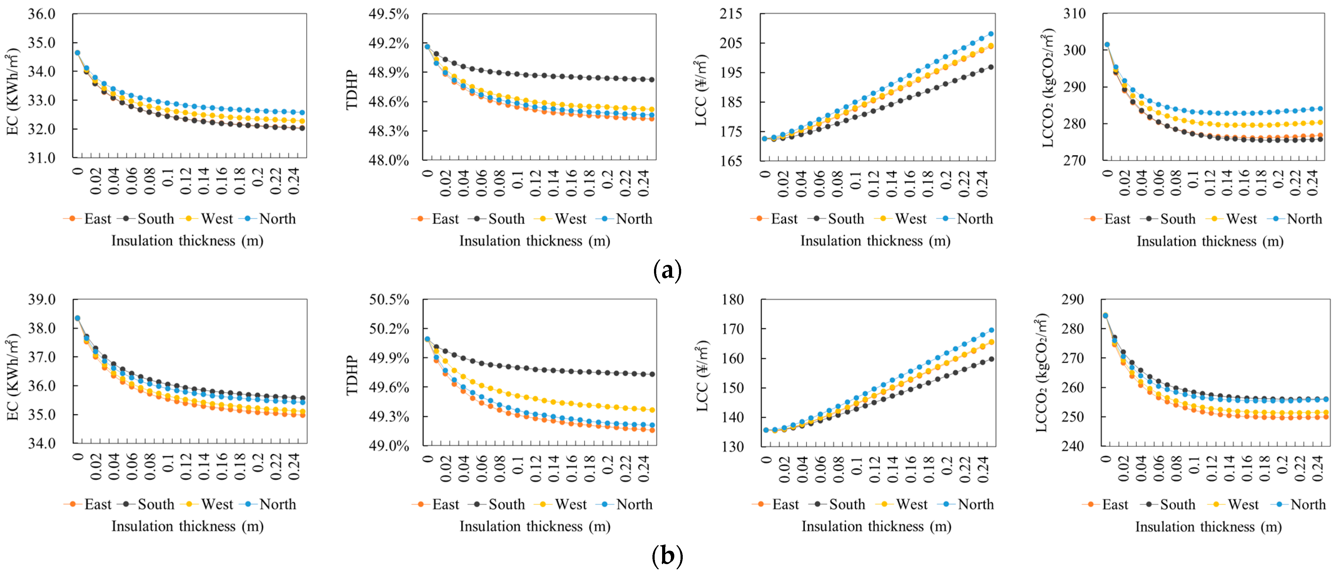
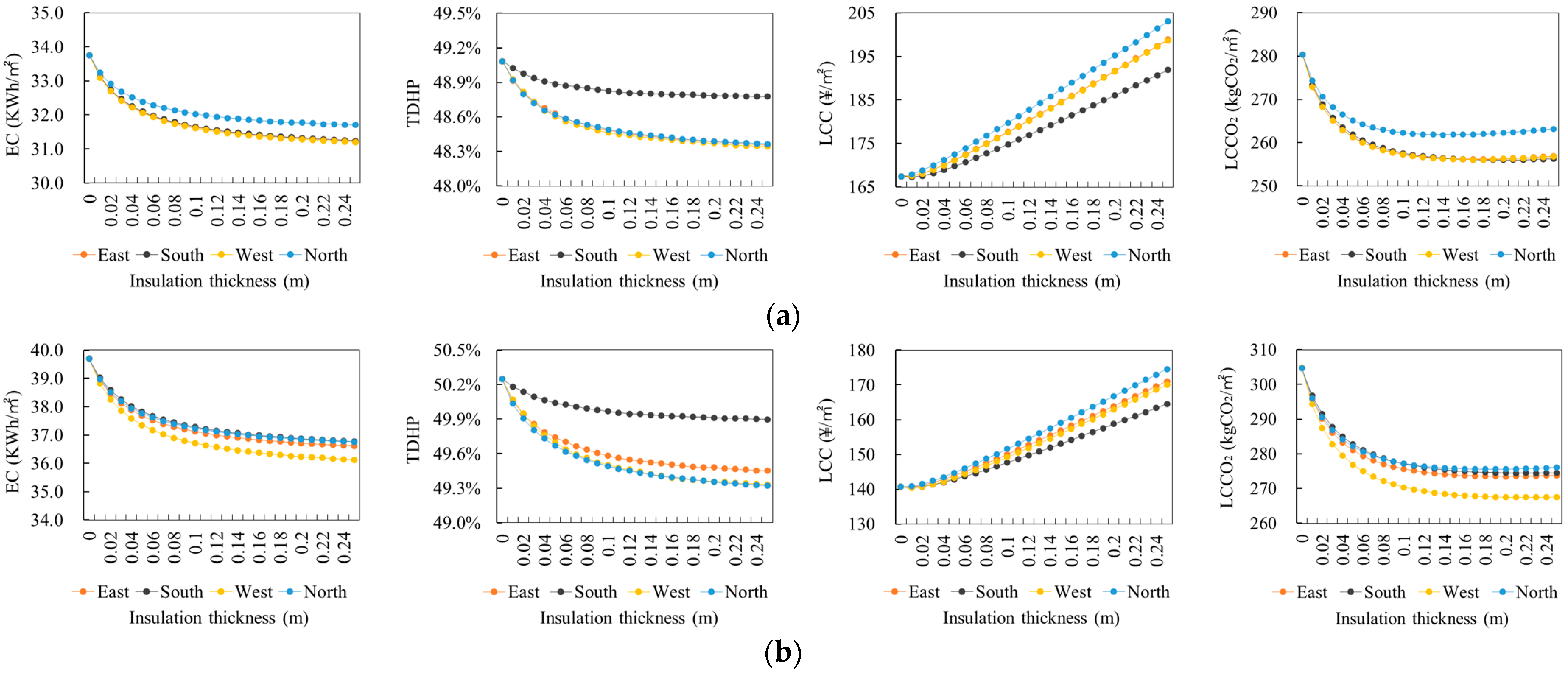
3.2.4. Effect of the External Wall’s Insulation Layer Thickness

Figure 15 displays the statistical results for the insulation layer thickness for external walls. The common characteristic is that, subject to the mutual restriction of the four objectives, the values are distributed over many points within the threshold, and there exist multiple extreme value points, whose corresponding insulation layer thicknesses are not exactly the same. This is different from the roof results, indicating that when considering multiple objectives comprehensively, a thicker external wall insulation layer is not better, and there is greater selectivity. Comparing the two regions, the average values of south, north, east, and west wall insulation layer thickness in Yulin are 0.13 m, 0.14 m, 0.13 m, and 0.13 m, respectively, which are higher than the values for Xi’an (0.12 m, 0.11 m, 0.12 m, and 0.09 m, respectively), and the differences reflected in the north and west wall insulation layer thickness are obvious. The mapping relationship between insulation layer thickness and the four objectives is analyzed below.

First of all, considering the influence of building orientation, two cases were set to analyze the relationship between insulation layer thickness and objective functions: ① the building orientation is to the south and ② the building orientation is south by west 30°. The simulation results of case-1 are shown in Figure 16. Firstly, with the increase in insulation layer thickness, EC and TDHP show a gradual decrease, LCC increases linearly, and LCCO₂ first presents a significant decrease and then a slow increase. Secondly, the change in the insulation layer thickness with different orientations has a diverse response degree to each objective. In the Xi’an area, the sensitivity order for EC is south wall ≈ east wall > west wall > north wall, for TDHP, it is east wall > north wall > west wall > south wall, for LCC, it is north wall > west wall ≈ east wall > south wall, and for LCCO₂, it is south wall ≈ east wall > west wall > north wall. Due to the different climate and solar radiation conditions, Yulin is essentially the same as Xi’an in terms of the influence rule, but there are differences in the response degree; for example, the sensitivity order for EC becomes east wall > west wall > north wall > south wall; for LCCO₂, it becomes east wall > west wall > north wall > south wall; and for TDHP and LCC, the sensitivity ranking remains unchanged.

The simulation results of case-2 are displayed in Figure 17. When the building orientation changes, the solar radiation heat gain of the four orientation walls will also be different. It can be observed from Figure 17 that the change rule of each objective with the increase in insulation layer thickness is consistent with case-1, but the response degree for some objectives is different. In the Xi’an area, the sensitivity ranking of EC is changed as follows: south wall (south by west 30°) ≈ east wall (east by north 30°) ≈ west wall (west by south 30°) > north wall (north by east 30°); for TDHP, it is east wall ≈ north wall ≈ west wall > south wall; and for LCCO₂, it is south wall ≈ east wall ≈ west wall > north wall. For the Yulin area, the sensitivity ranking of EC is changed as follows: west wall > east wall > north wall ≈ south wall; for TDHP, it is north wall > west wall ≈ east wall > south wall; for LCCO₂, it is west wall > east wall > south wall ≈ north wall. The ranking remains essentially unchanged for LCC in both regions.

Furthermore, the influence amplitude of the insulation layer thickness on the objective values will also change. Taking the south wall for example, in order to clearly reflect the comparison of two conditions, it is expressed by the difference in the value of objective functions between case-2 and case-1. As shown in Figure 18, for the Xi’an area, when the building orientation changes from south to 30° south by west, with an increase in insulation layer thickness, the influence amplitude on EC, LCC, and LCCO₂ essentially shows a decreasing trend, while that on TDHP displays a fluctuating state. For the Yulin area, the variation rule of influence amplitude is consistent, but in view of the objective values, the variation amplitude of EC and TDHP is higher than that for Xi’an, while that of LCC and LCCO₂ is lower. Therefore, when rotating the building orientation, the sensitivity and influence degree of the insulation layer thickness to the objectives will be changed. Different orientations corresponding to the optimal insulation thickness may also be different.

Furthermore, in view of the influence of exterior window type and window–wall ratio, taking the south wall of Xi’an as an example, based on the benchmark building, two cases were set as follows: ① the thermal performance of exterior windows is improved to type A and ② the south window–wall ratio is increased to 0.6. Figure 19 shows the variation curves of the objective functions’ difference values between case-1 and the benchmark building, and between case-2 and the benchmark building, with the insulation layer thickness. It can be seen that when the thermal performance of the exterior windows is improved, the variation range of EC and LCCO₂ shows an increasing trend, while that of TDHP and LCC decreases with the increase in insulation layer thickness. However, when the south window–wall ratio is increased, the variation range of EC and TDHP increases with the increase in insulation layer thickness, while LCC shows a trend of first decreasing and then increasing linearly, and LCCO₂ increases obviously at first and then decreases slightly. These results indicate that the effect amplitude of changing the insulation layer thickness on each objective is affected by the window type and area. This will also affect the determination of the optimal insulation layer thickness.

The above analysis shows that, unlike with single-objective optimization, a unique solution can be obtained. In the process of multi-objective optimization, due to the different action rules of design variables on each objective and the reciprocal effects of other variables, rich value possibilities are formed, which also provide more possibilities for the design scheme.

3.3. Optimal Design Solutions and Comparative Analysis of Different Regions

The optimized Pareto non-dominated solution set consists of a series of points, each of which is a solution associated with a set of decision variables representing the design scenario, all of which are acceptable. Associating the objective functions with design variables, the clustering parallel coordinate graphs are shown in Figure 20. It can be seen that it is impossible for all four objective values of any scheme to be better than those of the others; at least one objective will be unfavorable. Thus, these schemes are not directly comparable to one another. The corresponding design variable value is not the larger or smaller the better, but there is a coordination relationship with other variables. In order to verify the interpretability of the design variables to the objective functions and evaluate the robustness of the optimization results, the standard regression coefficient method was used for sensitivity analysis. The results show that the adjusted R² values for the four objectives of EC, TDHP, LCC, and LCCO₂ are 0.94, 0.93, 0.99, and 0.90 (Xi’an) and 0.93, 0.93, 0.99, and 0.90 (Yulin), respectively, with p < 0.01, indicating a very significant difference. It is evident that the design variables have a high degree of interpretation for the objective function, and the optimization results have high reliability, so they can be used for further analysis.

Different decision-makers may have different tendencies toward energy consumption, comfort demands, cost-effectiveness, and environmental impact, and they will ultimately need to adopt a decision method to determine the optimal design scheme. The TOPSIS decision-making method is used to make further comprehensive decisions to choose the optimal solutions from the Pareto solution set. Considering the balance of the four objectives, the scheme in which EC, LCC, TDHP, and LCCO₂ are equally important is the optimal scheme (case-1), so the weight value of each objective was set to 0.25. Meanwhile, the corresponding schemes where each objective is optimal were selected for comparison, i.e., EC optimal (case-2), TDHP optimal (case-3), LCC optimal (case-4), and LCCO₂ optimal (case-5).

Table 4. Optimal values of the objective functions and design parameters for Xi’an and Yulin.

Variables	Xi’an				Yulin
	Case-1	Case-2/ Case-5	Case-3	Case-4	Case-1	Case-2/ Case-5	Case-3	Case-4
O	25	30	25	25	10	5	5	0
Swwr	0.3	0.3	0.3	0.3	0.3	0.3	0.4	0.3
Nwwr	0.15	0.15	0.15	0.15	0.15	0.15	0.15	0.15
Swin	A	C	C	A	A	C	C	A
Nwin	B	C	C	A	C	C	C	A
St	0.2	0.2	0.18	0.02	0.17	0.17	0.17	0.02
Nt	0.1	0.17	0.16	0.05	0.15	0.2	0.2	0
Et	0.12	0.17	0.17	0.04	0.15	0.16	0.16	0.07
Wt	0.1	0.17	0.14	0.01	0.14	0.2	0.17	0.06
Rt	0.19	0.18	0.19	0.17	0.2	0.2	0.2	0.2
L	0.1	0	0.8	0.6	0.1	0	0	0.1
f1 (EC)	16.8	15.6	15.9	21.7	16.2	15.2	17.0	20.8
f2 (TDHP)	39.2%	38.6%	38.5%	40.5%	40.2%	39.8%	39.3%	42.1%
f3 (LCC)	254.8	314.4	305.8	199.3	230.2	272.7	291.8	165.2
f4 (LCCO2)	72.3	66.8	69.4	120.8	0	−7.0	45.2	44.5

Note: case-2 and case-5 are combined into a single column because they have the same solution.

indicates the optimal values of the objective functions and the corresponding design parameters of the four-objective optimization problem in Xi’an and Yulin.

As can be seen from Table 4 and Figure 5, case-1 is considered from the perspective of comprehensive performance and located in the middle region of the Pareto solution set. In the Xi’an area, the energy-saving rate of this scheme is 61.7% (the EC of the reference building is 43.9 KWh/m²), the TDHP improvement rate is 20.3% (the TDHP of the reference building is 49.2%), the LCC is 254.8 CNY/m², and the LCCO₂ is 72.3 kgCO₂/m². In the Yulin area, the corresponding values are 69.7% (the EC of the reference building is 53.4 KWh/m²), 19.4% (the TDHP of the reference building is 49.9%), 230.2 CNY/m², and 0 kgCO₂/m². Comparing the two regions, although the difference in building energy consumption is small, from the perspective of the energy-saving rate, the energy-saving potential of Yulin is higher, mainly because the region is rich in solar energy resources, and its photovoltaic power generation is significantly higher than that of Xi’an. If the photovoltaic power generation is not included, the energy-saving rate of the two regions is 39.2% and 41.2%, respectively; this difference is small, indicating that in the area of solar resource enrichment, the use of photovoltaic power generation can effectively reduce buildings’ energy consumption. The TDHP of Yulin is slightly higher than that of Xi’an, while the opposite is true for LCC and LCCO₂. It is worth noting that the LCCO₂ in Yulin has reached zero carbon. Corresponding to the values of the design variables, the building orientation in the two regions is different. According to the analysis in Section 3.2, both are in the optimal range conducive to reducing energy consumption. The south and north window–wall ratios, south external window type, and sunvisor overhang length are consistent. The thermal performance of the north exterior window and the insulation layer thickness of the exterior wall and roof in Yulin are greater than those in Xi’an, because of lower temperatures.

For the Xi’an region, case-2 has the lowest EC and case-5 has the lowest LCCO₂, both of which are the same scheme. This is mainly because carbon emissions are comprise material carbon emissions and operating carbon emissions, of which the latter occupy a large proportion, so they are greatly affected by buildings’ energy consumption. This can also be reflected by the scatter relationship between EC and LCCO₂ in Figure 5. Compared with case-1, the energy-saving rate increased by 2.8%, LCCO₂ decreased by 5.5 kgCO₂/m², TDHP decreased by 0.6%, and LCC increased by 59.6 CNY/m². For case-3, TDHP has the lowest value, and compared with case-1, the TDHP is reduced by 0.7%, the energy-saving rate is increased by 2.1%, LCCO₂ is reduced by 2.9 kgCO₂/m², and LCC is increased by 51 CNY/m². The LCC of case-4 has the lowest value, which is 55.5 CNY/m² lower than that of case-1, while its energy-saving rate is reduced by 5.7%, its TDHP is increased by 1.3%, and its LCCO₂ is increased by 48.5 kgCO₂/m². For the Yulin region, case-2 and case-5 are also the same scheme. Compared with case-1, the energy-saving rate is increased by 1.8%, LCCO₂ is reduced by 7.0 kgCO₂/m², TDHP is reduced by 0.4%, and LCC is increased by 42.5 CNY/m². For case-3, TDHP is decreased by 0.9%, the energy-saving rate is decreased by 1.5%, LCCO₂ is increased by 45.2 kgCO₂/m², and LCC is increased by 61.6 CNY/m². In case-4, LCC is reduced by 65 CNY/m², the energy-saving rate is reduced by 8.7%, TDHP is increased by 1.9%, and LCCO₂ is increased by 44.5 kgCO₂/m². Comparing the two regions, cases-2, -4, and -5 have a consistent change trend for each objective compared with case-1, while in case-3, the change trend of LCC is consistent but that of EC and LCCO₂ is the opposite, which is mainly related to the solar radiation. Because of the cold climate and abundant solar energy resources in Yulin, in order to improve indoor thermal comfort, it can be seen from the value of the design variable in case-3 that the south window–wall ratio is increased to 0.4, which is not conducive to reducing buildings’ energy consumption. Moreover, the available area of photovoltaic panels is reduced, which is not conducive to the power generation and carbon sink of renewable energy. Therefore, in terms of optimal indoor thermal comfort, EC and LCCO₂ are higher than in case-1. From the values of the design variables, there are also differences in the value characteristics formed under different preference guidance, such as in the optimal schemes of EC, LCCO₂, or TDHP, where the thermal performance of the south and north exterior windows and external walls is better than that of case-1. For the optimal LCC scheme, the thermal performance of the north exterior window and exterior wall is lower than that of case-1.

3.4. Comparison of Findings with Existing Studies, Applications, and Limitations

In the previous literature review, a broader scope was discussed, including research on multi-objective optimization of high-rise, multi-story, and low-rise residential buildings. This section focuses on the detailed comparison of related studies on high-rise buildings, taking [14,15,21,22] for example, as shown in

Table 5. Comparison with the existing studies on high-rise residential buildings.

Literature	Climatic Zone	Objectives	Design Variables	Consider PV?
[14]	Hot summer and cold winter zone	Energy consumption and indoor thermal comfort	Layout plans, orientation, shape coefficient, floor area, stories, north/south/west/east window–wall ratio, wall/roof/window heat transfer coefficient, and wall/roof heat inertia index	No
[15]	Cold zone	Heating energy consumption and discomfort hours in summer	Wall/roof insulation thickness, window type, gas tightness, horizontal sunvisor, and equipment system type	No
[21]	Severe cold, cold, hot summer and cold winter, hot summer and warm winter, mild zone	LCC and primary energy consumption	Wall/roof/window heat transfer coefficient, and total heat recovery efficiency	No
[22]	Severe cold zone	LCC and LCCO2	Wall/roof insulation thickness, window type, south/north/west/east window–wall ratio, and overhang depth, orientation	No

.

In comparison with the existing studies shown in Table 5, the contributions of our work are mainly twofold: firstly, the synchronous effects of four objectives are weighed by using the proposed method, as well as obtaining the Pareto solution set and optimal design solutions; secondly, the utilization of solar photovoltaic energy is considered in the objective function calculation, enabling a more comprehensive assessment of energy efficiency design, and the influence of differences in solar radiation is analyzed. For the different climate zones, such as in [14,22], the findings obtained are obviously different. Our findings are mainly comparable to those in [15,21], with the same climate region as our study. In [15], the heating energy consumption and summer uncomfortable hours were taken as optimization objectives in the preliminary screening, without considering the cost and carbon emissions. According to the tradeoff optimal solution obtained, compared with case-1 (Xi’an), the roof insulation layer is thicker and the window performance is better. In [21], the LCC and primary energy consumption were set as the optimization objectives, without considering thermal comfort and carbon emissions. Similarly, in the obtained equilibrium solution, the thermal performance of the exterior wall, roof, and exterior window was better than that of case-1 (Xi’an). This indicates that when the constraints are less, the values of design variables may have adverse effects on other objectives. In addition, the photovoltaic system in the present study was adopted to supplement the energy consumption; thus, our building energy-saving rate was higher than that in [17,23]. The utilization of renewable energy is indispensable.

It should be noted that only typical cases were selected above for contrastive analysis, and in practical applications the optimal scheme can be selected from the Pareto solution set according to the specific weight value of each objective. However, in the actual project design, the challenge is that some objectives or variables will be limited, so not all of the schemes in the Pareto solution set are applicable, and alternative schemes need to be screened out first. For optimization objectives, if the energy-saving rate is limited to a range, the schemes meeting the energy-saving requirements can be screened from the Pareto solution set first, and then the TOPSIS method can be used to determine the optimal scheme. Design variable values may also be constrained; for example, when the selection of building orientation is limited by the surrounding environment, it can be determined first, and then the best scheme can be determined from among the orientation options. Similarly, when constrained by multiple conditions, the optimal scheme can be determined step by step, starting from the restricted objective or variable. The priority order can also be given in combination with the entropy value proposed in Section 3.1. In the future, a user-friendly interface could be developed to facilitate operations and filter related parameters.

In addition, although the above findings can provide a basis for design practice, there are several limitations that need to be noted. Firstly, considering the shielding effect of the surrounding buildings against solar radiation, we chose the residence in the middle of the building group as the research object, but buildings in the first row, which are unshielded, will receive more solar radiation. Secondly, the utilization of solar radiation considered in this paper is an ideal state, which takes the building as a whole, assuming that the south facade is laid with photovoltaic panels except for the windows, but some locations on the facade receive less solar radiation and will not be laid with photovoltaic panels in reality, so the photovoltaic power generation and carbon sink will be reduced. Thirdly, our analysis was confined to a single climate zone. This research will be expanded to multiple climate zones to provide further reference for more regional building design.

4. Conclusions

This paper, focused on high-rise residential buildings located in two areas of Northwestern China with different solar radiation, introduces a multi-objective optimization method, which was implemented through the Grasshopper simulation and optimization platform coupled with a TOPSIS method to find the optimal design solution that minimized the EC, TDHP, LCC, and LCCO₂. A series of Pareto non-dominated solutions were identified. The main conclusions are as follows:

The optimization generated 65 and 82 Pareto-optimal solutions in total that significantly improved the four objectives for Xi’an and Yulin, respectively. From the comparison of the two cities, in terms of the relationship between building energy consumption and the other three objectives, the Pareto solution set in Yulin showed a more dispersed distribution, showing multiple approximately parallel curves.

This is mainly because the objective function considers the offset of solar power generation, and the solar radiation in Yulin is stronger, leading to different solution set distribution characteristics from those in Xi’an. This is mainly due to the fact that solar power generation is considered in the objective function calculation, and the solar radiation in Yulin is stronger, thus forming a solution set distribution characteristic different from that in Xi’an. From the perspective of objective value distribution, the LCC and LCCO₂ in Yulin have a wide distribution range, and the LCCO₂ is also negative due to the carbon reduction effect of photovoltaic power generation. However, the distribution of EC and TDHP is similar to that in Xi’an. In the value distribution of the four objectives, LCC has the largest distribution interval, followed by LCCO₂ and EC, while TDHP has the smallest span, indicating that the adjustment of design variables has a significant impact on the first three objectives, while the effect on TDHP is relatively small.

According to the value distribution of the design variables, as well as the quantitative relationship between the design variables and each objective, the value distribution characteristics of the design variables are different due to the constraints of the four objectives. Within a given threshold, the values of some variables are centrally distributed, such as the building orientation, which is concentrated in the middle. The value range of Xi’an is 20–30° south by west, while that of Yulin is 0°–15° south by west. The south and north window–wall ratios are concentrated at the lower limit of the threshold. The thickness of the roof insulation layer is mainly concentrated in the upper limit of the threshold. The values of the other variables are discretized, such as the sunvisor overhang length, but Yulin is different from Xi’an in that they are concentrated at the lower limit of threshold. The south and north exterior window types, along with the thickness of the external wall insulation layer, are discretionally distributed. These can also be reflected in the clustering parallel coordinate graph of the optimization objectives and variables. The reason for these conditions is that the design variables have different influence rules on each objective and, affected by the differences in climate conditions and solar radiation, these mechanisms will change. Even for the same region, when other design variables change, it will affect the influence degree of some design variables on the optimization objective.

The Pareto non-dominated solution set provides enough schemes for designers. The TOPSIS method was adopted to obtain the optimal scheme, from the perspective of comprehensive performance, with an energy-saving rate of 61.7%, TDHP improvement rate of 20.3%, LCC of 254.8 CNY/m², and LCCO₂ of 72.3 kgCO₂/m² in the Xi’an area. The corresponding values in the Yulin area are 69.7%, 19.4%, 230.2 CNY/m², and 0 kgCO₂/m². It can be seen that the energy-saving and carbon emission potential of Yulin is higher, mainly due to the abundant solar energy resources, photovoltaic power generation, and carbon sink being significantly higher than those of Xi’an. If the use of solar energy is excluded, the difference in the energy-saving rate between two regions is small. Meanwhile, the corresponding schemes when each objective is optimal were selected to compare with the optimal scheme. The results showed that climate condition, solar radiation, and the preference of optimization objective will affect the values of the objective functions and design variables.

The proposed method and the optimal solution sets obtained herein will provide references for high-rise residential building policy and practice in Northwestern China and other places with similar conditions. Moreover, this method can be applied to other types of buildings and climate zones. In future studies, a broader range of locations will be investigated, so as to provide more generalizable results. In terms of the subject, the design parameters of the building group will be taken as the variables, and the influence of building layout on solar radiation and energy consumption will be considered more accurately. Meanwhile, more indicators, such as natural lighting and ventilation, will be considered as the building performance optimization objectives, so as to make the optimization results more precise.

References

1. Sun, Y.; Wilson, R.; Wu, Y. A Review of Transparent Insulation Material (TIM) for building energy saving daylight comfort. Appl. Energy 2018, 226, 713–729. [Google Scholar] [CrossRef]
2. Javid, A.S.; Aramoun, F.; Bararzadeh, M.; Avami, A. Multi objective planning for sustainable retrofit of educational buildings. J. Build. Eng. 2019, 24, 100759. [Google Scholar] [CrossRef]
3. Ebrahimi-Moghadam, A.; Ildarabadi, P.; Aliakbari, K.; Fadaee, F. Sensitivity analysis and multi-objective optimization of energy consumption and thermal comfort by using interior light shelves in residential buildings. Renew. Energy 2020, 159, 736–755. [Google Scholar] [CrossRef]
4. Building Energy Efficiency Research Center, Tsinghua University (BEERC, TU). Annual Research Report on the Development of China Building Energy Efficiency; China Architecture & Building Press: Beijing, China, 2024. [Google Scholar]
5. Dong, H.; Qi, S.; Xu, M.; Ge, Z. Similarities and Differences of Effect of Wall Insulation on Energyconsumption of Residential Building in Cold Zone and Hot Summerand Cold Winter Zone. Ind. Constr. 2017, 47, 65–69. [Google Scholar] [CrossRef]
6. Chen, H.; Guo, J.; Jia, Y.; Du, T. Influence of Building Energy-Saving Parameters on Annual Heat Consumption. J. Build. Energy Effic. 2018, 46, 90–94. [Google Scholar] [CrossRef]
7. Zhu, L.; Shao, Z.; Sun, Y.; Zhu, J.; Cheng, S. Quantitative Research on Energy Efficiency Optimization of High-rise Residence in Zhengzhou. J. Build. Energy Effic. 2016, 44, 100–103. [Google Scholar]
8. Ascione, F.; De Masi, R.F.; De Rossi, F.; Ruggiero, S.; Vanoli, G.P. Optimization of Building Envelope Design for nZEBs in Mediterranean Climate: Performance Analysis of Residential Case Study. Appl. Energy 2016, 183, 938–957. [Google Scholar] [CrossRef]
9. Li, J. Coordination and Optimization of Envelope Key Parameters for Nearly Zero Energy High-Rise Residence in Cold Region. Master’s Thesis, Shandong Jianzhu University, Jinan, China, 2018. [Google Scholar]
10. Mao, P.; Yang, L.; Luo, Z. Life-cycle Carbon Emission Assessment Method of Building Constructions: Taking the Wall Constructions of Residential Buildings in Xi’an as Examples. Huazhong Archit. 2019, 37, 32–37. [Google Scholar]
11. GB/T 51350-2019; Ministry of Housing and Urban-Rural Development of PRC (MOHURD). Technical Standard for Nearly Zero Energy Buildings. China Architecture & Building Press: Beijing, China, 2019.
12. Deng, F.; Tang, H. Research on Energy Consumption and Photovoltaic Substitution Rate of Different Types of Residence in Shanghai Based on Nearly Zero Energy Consumption. Build. Sci. 2021, 37, 9–18. [Google Scholar] [CrossRef]
13. Chen, X.; Wang, Q.; Srebric, J. Model predictive control for indoor thermal comfort and energy optimization using occupant feedback. Energy Build. 2015, 102, 357–369. [Google Scholar] [CrossRef]
14. Yu, W.; Li, B.; Jia, H.; Zhang, M.; Wang, D. Application of multi-objective genetic algorithm to optimize energy efficiency and thermal comfort in building design. Energy Build. 2015, 88, 135–143. [Google Scholar] [CrossRef]
15. Wu, D.; Liu, L.; Li, X.; Liu, C. Research on the Technologies of Passive Low Energy Buildings on the Basis of Multi-Objective Optimization Method—By Taking Cold Zone Residential Buildings for Example. J. S. China Univ. Technol. Nat. Sci. Ed. 2018, 46, 98–104,120. [Google Scholar] [CrossRef]
16. Fabrizio, A.; Nicola, B.; De Masi, R.F.; Mauro, G.M.; Vanoli, G.P. Design of the Building Envelope: A Novel Multi-Objective Approach for the Optimization of Energy Performance and Thermal Comfort. Sustainability 2015, 7, 10809–10836. [Google Scholar] [CrossRef]
17. Bre, F.; Roman, N.; Fachinotti, V.D. An efficient metamodel-based method to carry out multi-objective building performance optimizations. Energy Build. 2020, 206, 109576. [Google Scholar] [CrossRef]
18. Gao, Y.; Hu, K.; Yue, X.; Yuan, J. Shape Parameters Design of Northern Rural Houses for Multi-Objective Optimization of Energy Performance and Thermal Comfort. J. Huaqiao Univ. Nat. Sci. 2021, 42, 619–627. [Google Scholar]
19. Pal, S.K.; Takano, A.; Alanne, K.; Palonen, M.; Siren, K. A multi-objective life cycle approach for optimal building design: A case study in Finnish context. J. Clean. Prod. 2016, 143, 1021–1035. [Google Scholar] [CrossRef]
20. Harkouss, F.; Fardoun, F.; Biwole, P.H. Multi-Objective Optimization Methodology for Net Zero Energy Buildings. J. Build. Eng. 2018, 16, 57–71. [Google Scholar] [CrossRef]
21. Yu, Z.; Lu, F.; Zou, Y.; Xu, W.; Sun, D.; Liu, C. A Simulation-based Multi-objective Optimization Approach for Design of Nearly Zero Energy Buildings. Build. Sci. 2019, 35, 8–15. [Google Scholar] [CrossRef]
22. Xue, Q.; Wang, Z.; Chen, Q. Multi-objective optimization of building design for life cycle cost and CO2 emissions: A case study of a low-energy residential building in a severe cold climate. Build. Simul. 2022, 15, 83–98. [Google Scholar] [CrossRef]
23. Li, K.; Pan, L.; Xue, W.; Jiang, H.; Mao, H. Multi-Objective Optimization for Energy Performance Improvement of Residential Buildings: A Comparative Study. Energies 2017, 10, 245. [Google Scholar] [CrossRef]
24. Ascione, F.; Bianco, N.; Mauro, G.M.; Napolitano, D.F. Building envelope design: Multi-objective optimization to minimize energy consumption, global cost and thermal discomfort. Application to different Italian climatic zones. Energy 2019, 174, 359–374. [Google Scholar] [CrossRef]
25. Abdou, N.; ELMghouchi, Y.; Hamdaoui, S.; ELAsri, N.; Mouqallid, M. Multi-objective optimization of passive energy efficiency measures for net-zero energy building in Morocco. Build. Environ. 2021, 204, 108141. [Google Scholar] [CrossRef]
26. Jung, Y.; Heo, Y.; Lee, H. Multi-objective optimization of the multi-story residential building with passive design strategy in South Korea. Build. Environ. 2021, 203, 108061. [Google Scholar] [CrossRef]
27. Jin, G.; Ma, J.; Yang, P.; Chen, W. MABC-BPNN based multi-objective optimization prediction model for ultra.low energy consumption residential houses in western Inner Mongolia Grassland. J. Arid. Land Resour. Environ. 2021, 35, 73–79. [Google Scholar] [CrossRef]
28. Li, Z.; Shi, X.; Tian, M. Research on Climate Responsive Optimisation Design of Residential Buildings. S. Archit. 2022, 210, 8–16. [Google Scholar]
29. Gao, Y.; Luo, S.; Chi, J.; Yuan, J. A Multi-objective Optimisation Evaluation Method for the Low-carbon Renovation of Rural Houses. S. Archit. 2022, 4, 61–68. [Google Scholar] [CrossRef]
30. Standard 140-2007; ANSI/ASHRAE. Standard Method of Test for the Evaluation of Building Energy Analysis Computer Programs, American Society of Heating, Refrigerating and Air-Conditioning Engineers. ASHRAE: Atlanta, GA, USA, 2007.
31. Delgarm, N.; Sajadi, B.; Delgarm, S.; Kowsary, F. A novel approach for the simulation-based optimization of the building’s energy consumption using NSGA-II: Case study in Iran. Energy Build. 2016, 127, 552–560. [Google Scholar] [CrossRef]
32. Krzysztof, G.; Joanna, F.G. Multi-Objective Optimization of the Envelope of Building with Natural Ventilation. Energies 2018, 11, 1383. [Google Scholar] [CrossRef]
33. Hong, T.; Kim, J.; Lee, M. A multi-objective optimization model for determining the building design and occupant behaviors based on energy, economic, and environmental performance. Energy 2019, 174, 823–834. [Google Scholar] [CrossRef]
34. Shao, T.; Zheng, W.; Jin, H. Analysis of the Indoor Thermal Environment and Passive Energy-Saving Optimization Design of Rural Dwellings in Zhalantun, Inner Mongolia, China. Sustainability 2020, 12, 1103. [Google Scholar] [CrossRef]
35. Kheiri, F. A review on optimization methods applied in energy-efficient building geometry and envelope design. Renew. Sustain. Energy Rev. 2018, 92, 897–920. [Google Scholar] [CrossRef]
36. Zitzler, E.; Laumanns, M.; Thiele, L. SPEA2: Improving the strength pareto evolutionary algorithm. Tech. Rep. Gloriastrasse 2001, 103, 1–21. [Google Scholar] [CrossRef]
37. Zhang, A.; Bokel, R.; Andy, V.D.D.; Sun, Y.; Huang, Q.; Zhang, Q. Optimization of thermal and daylight performance of school buildings based on a multi-objective genetic algorithm in the cold climate of China. Energy Build. 2017, 139, 371–384. [Google Scholar] [CrossRef]
38. Ghasemi, K.; Hamzenejad, M.; Meshkini, A. An analysis of the spatial distribution pattern of social-cultural services and their equitable physical organization using the TOPSIS technique: The case-study of Tehran, Iran. Sustain. Cities Soc. 2019, 51, 101708. [Google Scholar] [CrossRef]
39. Kokaraki, N.; Hopfe, C.J.; Robinson, E.; Nikolaidou, E. Testing the reliability of deterministic multi-criteria decision-making methods using building performance simulation. Renew. Sustain. Energy Rev. 2019, 112, 991–1007. [Google Scholar] [CrossRef]
40. GB 50176-2016; Ministry of Housing and Urban-Rural Development of PRC (MOHURD). Thermal Design Code for Civil Building. China Architecture & Building Press: Beijing, China, 2016.
41. GB 50180-2018; Ministry of Housing and Urban-Rural Development of PRC (MOHURD). Standard for Urban Residential Area Planning and Design. China Architecture & Building Press: Beijing, China, 2018.
42. Picco, M.; Marengo, M. On the Impact of simplifications on Building Energy Simulation for Early Stage Building Design. J. Eng. Archit. 2015, 3, 68–77. [Google Scholar] [CrossRef]
43. JGJ26-2018; Ministry of Housing and Urban-Rural Development of PRC (MOHURD). Design Standard for Energy Efficiency of Residential Buildings in Severe Cold and Cold Zones. China Architecture & Building Press: Beijing, China, 2018.
44. BS EN 15459-1; British Standards Institution (BSI). Energy Performance of Buildings—Economic Evaluation Procedure for Energy Systems in Buildings. BSI Standards Limited: London, UK, 2017.
45. Hasan, A.; Vuolle, M.; Siren, K. Minimization of life cycle cost of detached house using combined simulation and optimization. Build. Environ. 2008, 43, 2022–2034. [Google Scholar] [CrossRef]
46. Ren, H. Study of Indoor Thermal Comfort of Residential Buildings in Xi’an. Master’s Thesis, Xi’an University of Architecture and Technology, Xi’an, China, 2019. [Google Scholar] [CrossRef]
47. GB/T 51366-2019; Ministry of Housing and Urban-Rural Development of PRC (MOHURD). Standard for Building Carbon Emission Calculaiton. China Architecture & Building Press: Beijing, China, 2019.
48. Lei, Y.J.; Zhang, S.; Li, X.; Zhou, C.M. MATLAB Genetic Algorithm Toolbox and Application; Xidian University Press: Xi’an, China, 2005. [Google Scholar]
Figure 1. Overall workflow for the multi-objective optimization of high-rise residential buildings.
Applsci 14 06719 g001
Figure 2. Monthly average dry-bulb temperature of the two cities.
Applsci 14 06719 g002
Figure 3. Monthly total solar radiation of the two cities.
Applsci 14 06719 g003
Figure 4. (a) Layout of the benchmark building; (b) location of the research object in the residential area.
Applsci 14 06719 g004
Figure 5. The relationships between the bi-objective Pareto solutions at Xi’an and Yulin: (a) Xi’an; (b) Yulin.
Applsci 14 06719 g005
Figure 6. Value distribution of building orientation in Pareto solutions: (a) Xi’an and (b) Yulin.
Applsci 14 06719 g006
Figure 7. Relationship between building orientation, EC, and TDHP: (a) Xi’an and (b) Yulin.
Applsci 14 06719 g007
Figure 8. Value distribution of window–wall ratio and sunvisor overhang length in Pareto solutions: (a) Xi’an and (b) Yulin.
Applsci 14 06719 g008aApplsci 14 06719 g008b
Figure 9. Value distribution of window types in Pareto solutions: (a) Xi’an and (b) Yulin.
Applsci 14 06719 g009
Figure 10. Relationship between the south window–wall ratio and the four objectives in Xi’an: (a) case-1; (b) case-2; and (c) case-3.
Applsci 14 06719 g010
Figure 11. Relationship between the south window–wall ratio and the four objectives in Yulin: (a) case-1; (b) case-2; and (c) case-3.
Applsci 14 06719 g011
Figure 12. Relationship between the south sunvisor overhang length and the four objectives in Xi’an: (a) case-1; (b) case-2; and (c) case-3.
Applsci 14 06719 g012
Figure 13. Value distribution of roof insulation layer thickness in Pareto solutions: (a) Xi’an and (b) Yulin.
Applsci 14 06719 g013
Figure 14. Relationship between roof insulation layer thickness and four objectives: (a) Xi’an and (b) Yulin.
Applsci 14 06719 g014
Figure 15. Value distribution of insulation layer thickness for external walls in Pareto solutions: (a) Xi’an and (b) Yulin.
Applsci 14 06719 g015
Figure 16. Relationship between external wall insulation layer thickness and four objectives (case-1): (a) Xi’an and (b) Yulin.
Applsci 14 06719 g016
Figure 17. Relationship between external wall insulation layer thickness and four objectives (case-2): (a) Xi’an and (b) Yulin.
Applsci 14 06719 g017
Figure 18. Relationship between south wall insulation layer thickness and difference values of objective functions: (a) Xi’an and (b) Yulin.
Applsci 14 06719 g018
Figure 19. Variation curve of objective functions’ difference values between case-1, case-2, and the benchmark building: (a) Case-1 and (b) Case-2.
Applsci 14 06719 g019
Figure 20. Optimization objectives and variables clustered in a parallel coordinate graph (1, 2, and 3 correspond to window types A, B, and C, respectively). (a) Xi’an and (b) Yulin.
Applsci 14 06719 g020