
A New Shear Wave Velocity-Based Liquefaction Probability Model Using Logistic Regression: Emphasizing Fines Content Optimization
Abstract
:1. Introduction
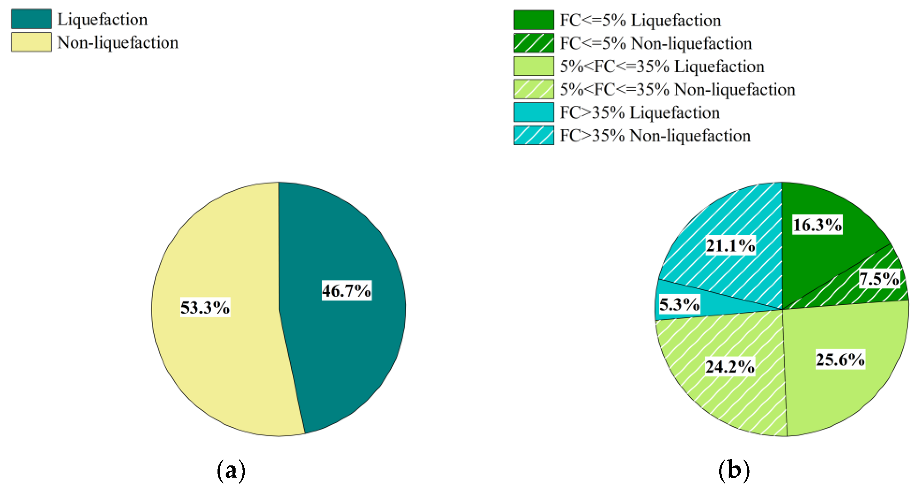
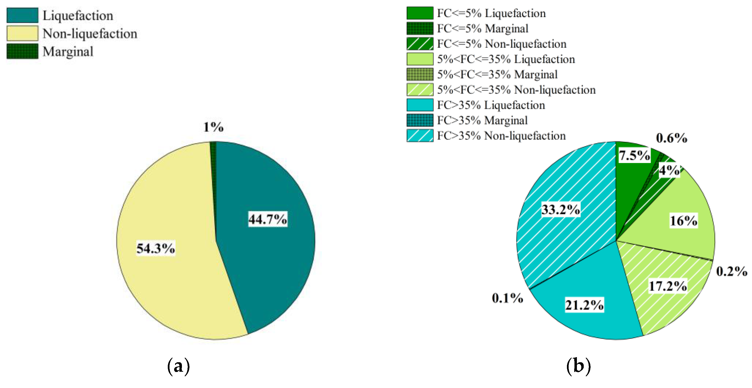
2. Data
3. Comparative Analysis of Existing Evaluation Methods
3.1. Existing Evaluation Methods
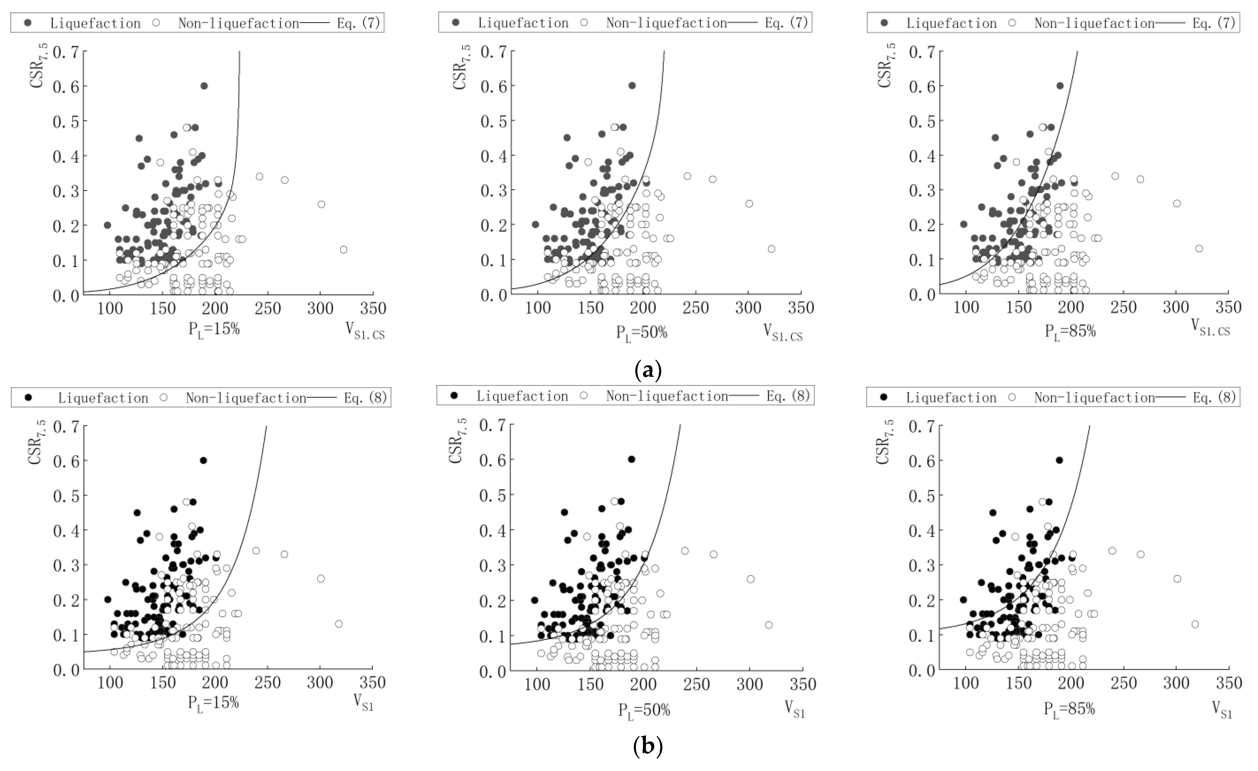
3.1.1. Juang’s Liquefaction Probability Assessment Method
3.1.2. Kayen’s Liquefaction Probability Assessment Method
3.1.3. Chen’s Liquefaction Probability Assessment Method
3.1.4. Cao’s Liquefaction Probability Assessment Method
3.1.5. Shen’s Liquefaction Probability Assessment Method
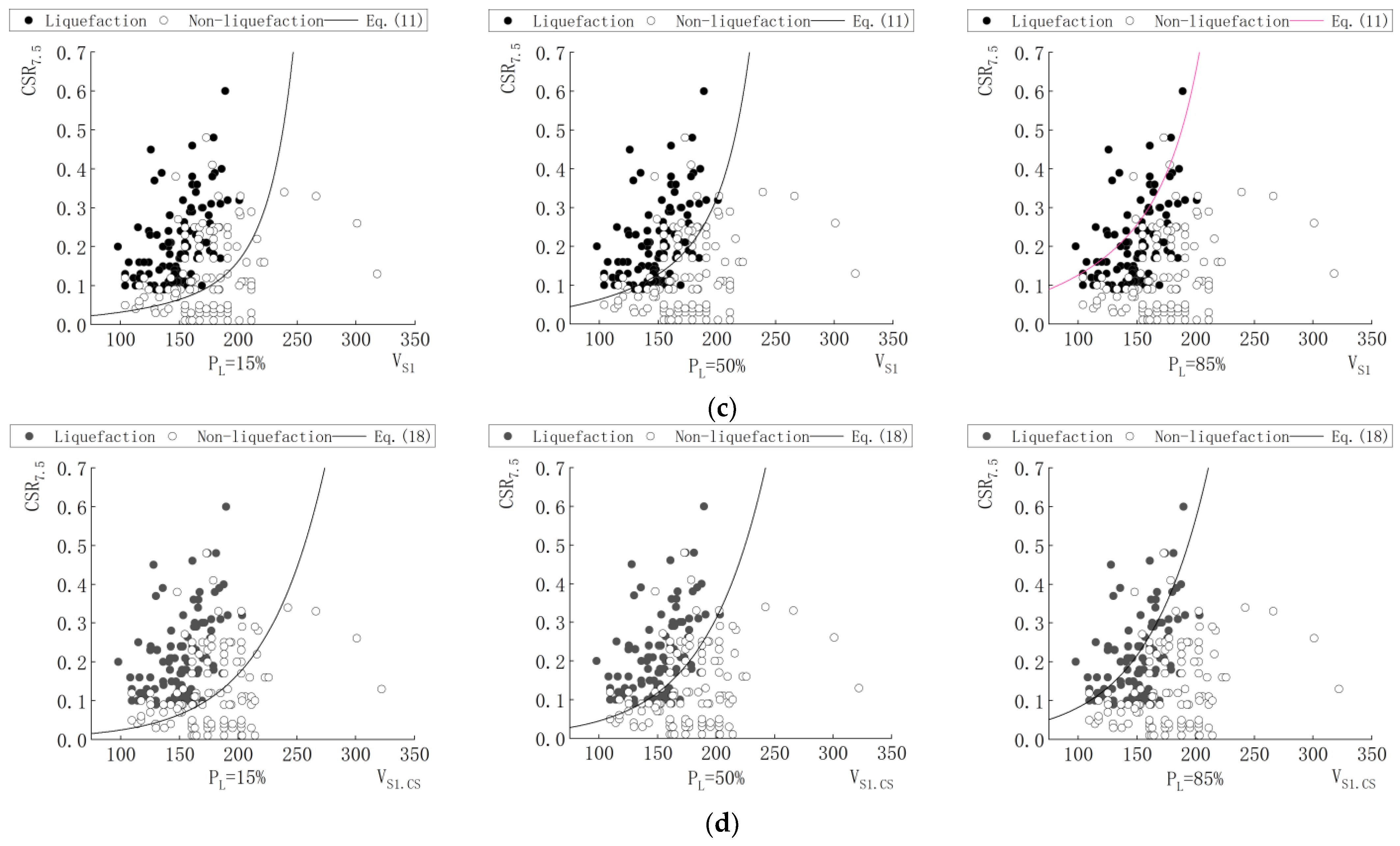
3.1.6. Rollins’ Liquefaction Probability Assessment Method
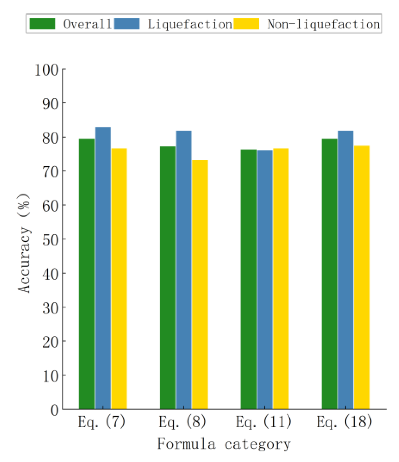
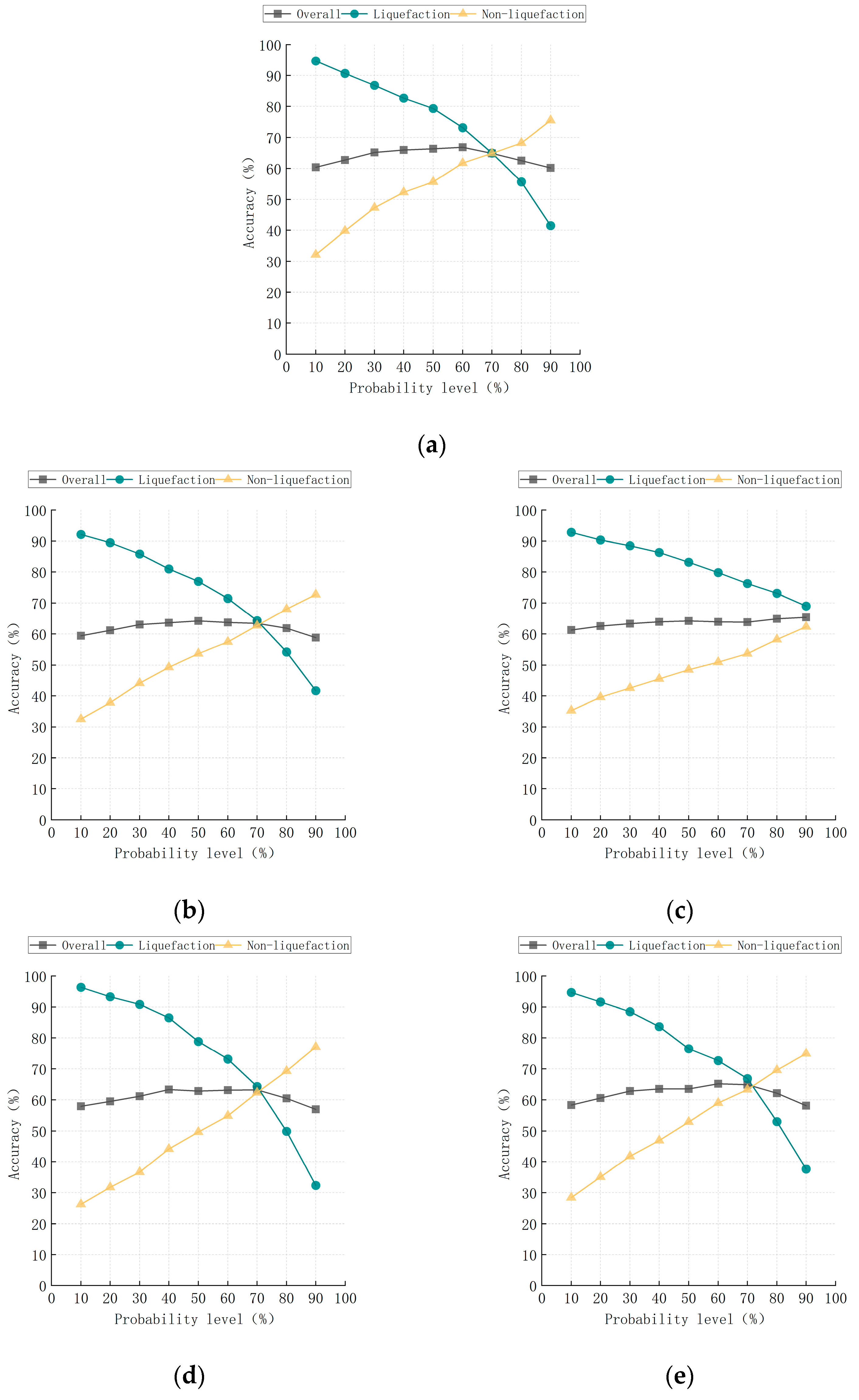
3.2. Overall Accuracy
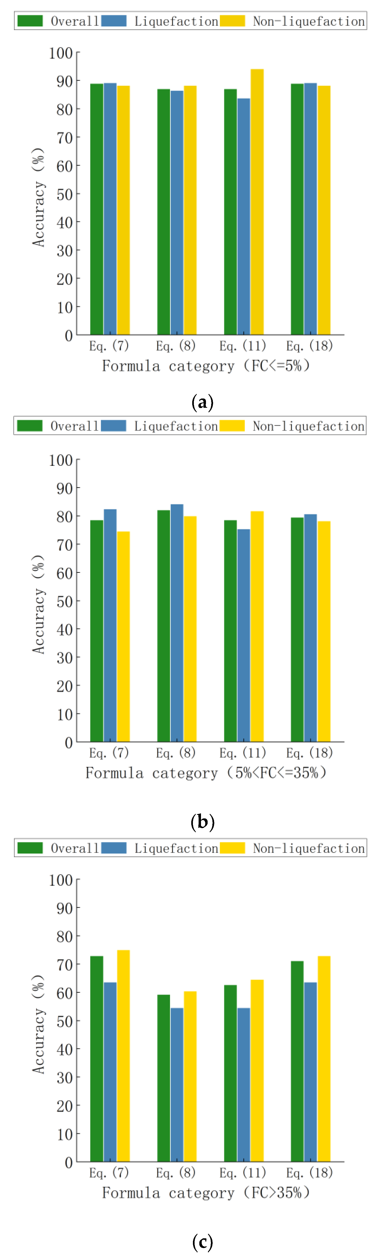
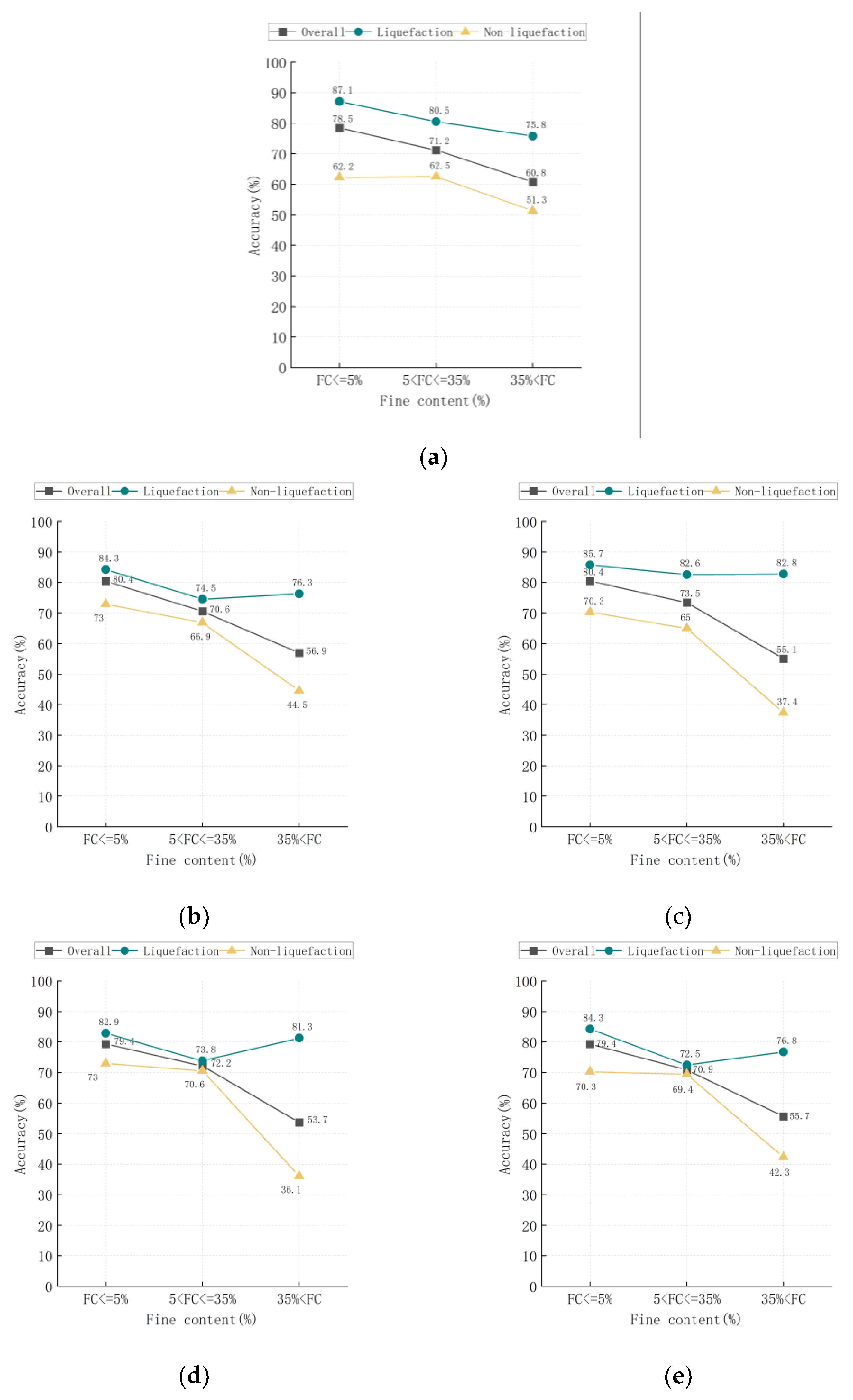
3.3. Accuracy for Different Levels of Fines Content
3.4. Applicability Analysis
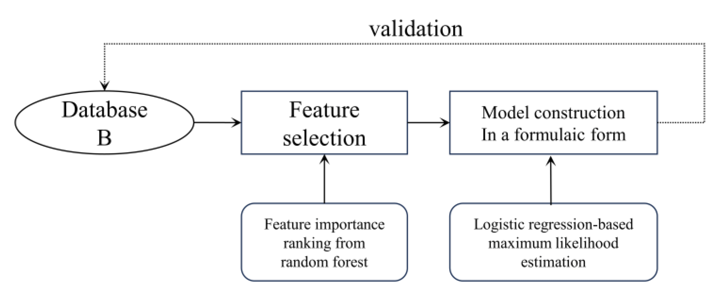
4. Development of LR Liquefaction Probability Model
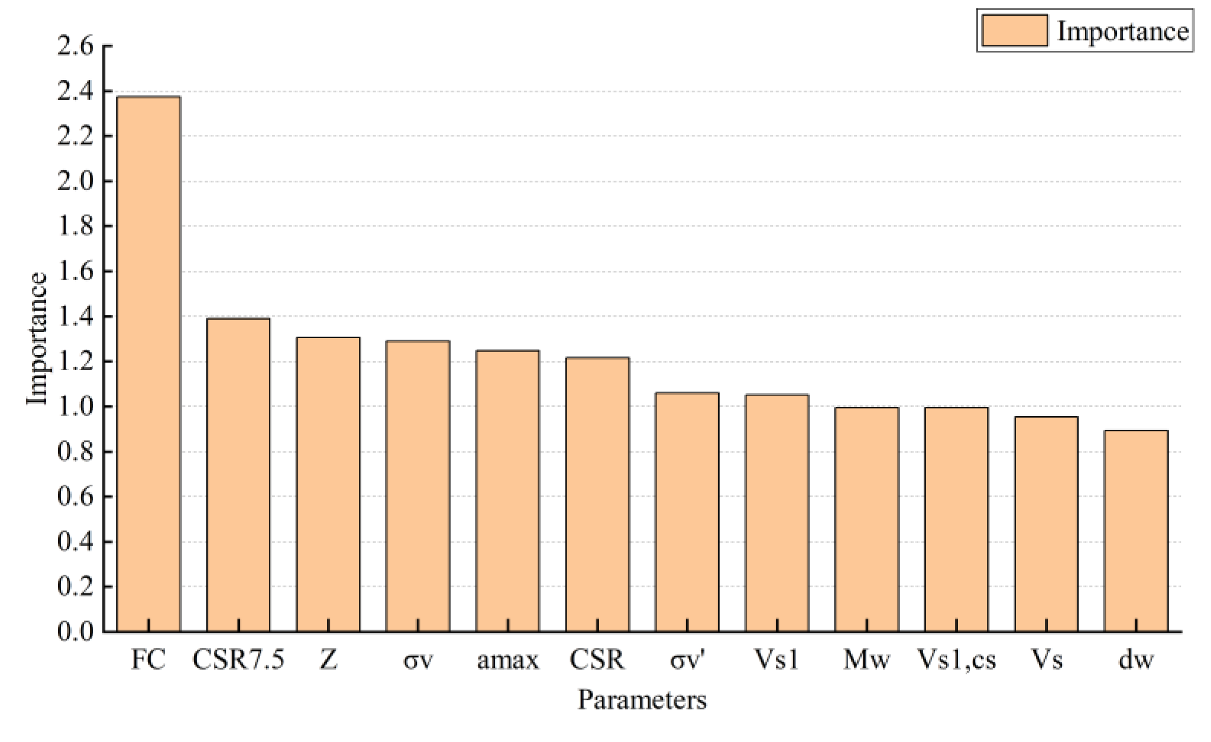
4.1. Feature Selection and Parameter Setting
4.2. Model Construction
5. Discussion of Results
6. Conclusions
Author Contributions
Funding
Institutional Review Board Statement
Informed Consent Statement
Data Availability Statement
Conflicts of Interest
Nomenclature
| amax | peak ground acceleration | Pa | standard atmospheric pressure |
| CSR | cyclic stress ratio | PL | liquefaction probability |
| CSR7.5 | CSR normalized to MW = 7.5 | Vs | shear wave velocity |
| CRR | cyclic resistance ratio | Vs1 | effective stress-normalized shear wave velocity |
| dw | groundwater level | Vs1,cs | clean sand equivalence of stress-corrected shear wave velocity |
| FC | fines content | Z | depth |
| FS | factor of safety | σv | vertical total stress |
| nominal safety factor | σv′ | vertical effective stress | |
| K | fines content correction | Φ | cumulative normal distribution function |
| MW | moment magnitude |
References
- Zhou, J.; Huang, S.; Zhou, T.; Armaghani, D.J.; Qiu, Y. Employing a genetic algorithm and grey wolf optimizer for optimizing RF models to evaluate soil liquefaction potential. Artif. Intell. Rev. 2022, 55, 5673–5705. [Google Scholar] [CrossRef]
- Castro, G. Liquefaction and cyclic mobility of saturated sands. J. Thegeotechnical Eng. Div. 1975, 101, 551–569. [Google Scholar] [CrossRef]
- Guo, H.; Zhao, J.X. The surface rupture zone and paleoseismic evidence on the seismogenic fault of the 1976 Ms 7.8 Tangshan earthquake, China. Geomorphology 2019, 327, 297–306. [Google Scholar] [CrossRef]
- Hu, J.L.; Tang, X.W.; Qiu, J.N. A Bayesian network approach for predicting seismic liquefaction based on interpretive structural modeling. Georisk Assess. Manag. Risk Eng. Syst. Geohazards 2015, 9, 200–217. [Google Scholar] [CrossRef]
- Vipin, K.S.; Sitharam, T.G.; Anbazhagan, P. Probabilistic evaluation of seismic soil liquefaction potential based on SPT data. Nat. Hazards 2010, 53, 547–560. [Google Scholar] [CrossRef]
- Mahmood, A.; Tang, X.W.; Qiu, J.N.; Gu, W.J.; Feezan, A. A hybrid approach for evaluating CPT-based seismic soil liquefaction potential using Bayesian belief networks. J. Cent. South Univ. 2020, 27, 500–516. [Google Scholar] [CrossRef]
- Hu, J.L.; Liu, H.B. Bayesian network models for probabilistic evaluation of earthquake-induced liquefaction based on CPT and Vs databases. Eng. Geol. 2019, 254, 76–88. [Google Scholar] [CrossRef]
- Rollins, K.M.; Roy, J.; Athanasopoulos-Zekkos, A.; Zekkos, D.; Amoroso, S.; Cao, Z. A new dynamic cone penetration test–based procedure for liquefaction triggering assessment of gravelly soils. J. Geotech. Geoenvironmental Eng. 2021, 147, 04021141. [Google Scholar] [CrossRef]
- Rollins, K.M.; Roy, J.; Athanasopoulos-Zekkos, A.; Zekkos, D.; Amoroso, S.; Cao, Z.; Milana, G.; Vassallo, M.; Di Giulio, G. A new V s-based liquefaction-triggering procedure for gravelly soils. J. Geotech. Geoenvironmental Eng. 2022, 148, 04022040. [Google Scholar] [CrossRef]
- Yang, H.; Liu, Z.; Xie, Y.; Li, S. A probabilistic liquefaction reliability evaluation system based on CatBoost-Bayesian considering uncertainty using CPT and Vs measurements. Soil Dyn. Earthq. Eng. 2023, 173, 108101. [Google Scholar] [CrossRef]
- Wang, T.; Xiao, S.; Zhang, J.; Zuo, B. Depth-consistent models for probabilistic liquefaction potential assessment based on shear wave velocity. Bull. Eng. Geol. Environ. 2022, 81, 255. [Google Scholar] [CrossRef]
- Andrus, R.D.; Stokoe, K.H. Liquefaction resistance of soils from shear-wave velocity. J. Geotech. Geoenvironmental Eng. 2000, 126, 1015–1025. [Google Scholar] [CrossRef]
- Hou, X.M.; Qu, S.Y.; Shi, X.D. Signal processing method for shear wave velocity measurement. Earthq. Eng. Eng. Vib. 2007, 6, 205–212. [Google Scholar] [CrossRef]
- Lu, C.C.; Hwang, J.H. Correlations between Vs and SPT-N by different borehole measurement methods: Effect on seismic site classification. Bull. Earthq. Eng. 2020, 18, 1139–1159. [Google Scholar] [CrossRef]
- Kayen, R.; Moss, R.E.S.; Thompson, E.M.; Seed, R.B.; Cetin, K.O.; Kiureghian, A.D.; Tanaka, Y.; Tokimatsu, K. Shear-wave velocity–based probabilistic and deterministic assessment of seismic soil liquefaction potential. J. Geotech. Geoenvironmental Eng. 2013, 139, 407–419. [Google Scholar] [CrossRef]
- Dobry, R.; Stokoe, K.H.; Ladd, R.S.; Youd, T.L. Liquefaction susceptibility from S-wave velocity. In Proceedings of the In-Situ Tests to Evaluate Liquefaction Susceptibility, ASCE National Convention, New York, NY, USA, 26–31 October 1981. [Google Scholar]
- Seed, H.B.; Idriss, I.M. Simplified procedure for evaluating soil liquefaction potential. J. Soil Mech. Found. Div. 1971, 97, 1249–1273. [Google Scholar] [CrossRef]
- Kayen, R.E.; Mitchell, J.K.; Seed, R.B.; Lodge, A.; Nishio, S.Y.; Coutinho, R. Evaluation of SPT-, CPT-, and shear wave-based methods for liquefaction potential assessment using Loma Prieta data. In Proceedings of the 4th Japan-US Workshop on Earthquake Resistant Design of Lifeline Facilities and Countermeasures for Soil Liquefaction, Buffalo, NY, USA, 19–21 August 1991. [Google Scholar]
- Robertson, P.K.; Woeller, D.J.; Finn WD, L. Seismic cone penetration test for evaluating liquefaction potential under cyclic loading. Can. Geotech. J. 1992, 29, 686–695. [Google Scholar] [CrossRef]
- Lodge, A.L. Shear Wave Velocity Measurements for Subsurface Characterization; University of California: Berkeley, CA, USA, 1994. [Google Scholar]
- Juang, C.H.; Chen, C.J.; Jiang, T. Probabilistic framework for liquefaction potential by shear wave velocity. J. Geotech. Geoenvironmental Eng. 2001, 127, 670–678. [Google Scholar] [CrossRef]
- Shen, M.; Chen, Q.; Zhang, J.; Gong, W.; Hsein Juang, C. Predicting liquefaction probability based on shear wave velocity: An update. Bull. Eng. Geol. Environ. 2016, 75, 1199–1214. [Google Scholar] [CrossRef]
- Li, P.; Tian, Z.; Bo, J.; Zhu, S.; Li, Y. Study on sand liquefaction induced by Songyuan earthquake with a magnitude of M5. 7 in China. Sci. Rep. 2022, 12, 9588. [Google Scholar]
- Lees, J.; Ballagh, R.; Orense, R.; van Ballegooy, S. CPT-based analysis of liquefaction and re-liquefaction following the Canterbury earthquake sequence. Soil Dyn. Earthq. Eng. 2015, 79, 304–314. [Google Scholar] [CrossRef]
- Zhou, Y.G.; Xia, P.; Ling, D.S.; Chen, Y.M. Liquefaction case studies of gravelly soils during the 2008 Wenchuan earthquake. Eng. Geol. 2020, 274, 105691. [Google Scholar] [CrossRef]
- Kumar, D.; Samui, P.; Kim, D.; Singh, A. A novel methodology to classify soil liquefaction using deep learning. Geotech. Geol. Eng. 2021, 39, 1049–1058. [Google Scholar] [CrossRef]
- Ahmad, M.; Tang, X.W.; Qiu, J.N.; Ahmad, F.; Gu, W.J. Application of machine learning algorithms for the evaluation of seismic soil liquefaction potential. Front. Struct. Civ. Eng. 2021, 15, 490–505. [Google Scholar] [CrossRef]
- Ozsagir, M.; Erden, C.; Bol, E.; Sert, S.; Özocak, A. Machine learning approaches for prediction of fine-grained soils liquefaction. Comput. Geotech. 2022, 152, 105014. [Google Scholar] [CrossRef]
- Moghaddam, A.; Barari, A.; Farahani, S.; Tabarsa, A.; Jeng, D.-S. Effective stress analysis of residual wave-induced liquefaction around caisson-foundations: Bearing capacity degradation and an AI-based framework for predicting settlement. Comput. Geotech. 2023, 159, 105364. [Google Scholar] [CrossRef]
- Andrus, R.D.; Stokoe, K.H., II; Chung, R.M. Draft Guidelines for Evaluating Liquefaction Resistance Using Shearwave Velocity Measurements and Simplified Procedures; US Department of Commerce, Technology Administration, National Institute of Standardsand Technology: Gaithersburg, MD, USA, 1999. [Google Scholar]
- Chu, B.L.; Hsu, S.C.; Chang, Y.M. Ground behavior and liquefaction analyses in central Taiwan-Wufeng. Eng. Geol. 2004, 71, 119–139. [Google Scholar] [CrossRef]
- Saygili, G. Liquefaction Potential Assessment in Soil Deposits Using Artificial Neural Networks; Concordia University: Montreal, QC, Canada, 2005. [Google Scholar]
- Cai, G.J.; Liu, S.Y.; Puppala, A.J. Liquefaction assessments using seismic piezocone penetration (SCPTU) test investigations in Tangshan region in China. Soil Dyn. Earthq. Eng. 2012, 41, 141–150. [Google Scholar] [CrossRef]
- Hanna, A.M.; Ural, D.; Saygili, G. Neural network model for liquefaction potential in soil deposits using Turkey and Taiwan earthquake data. Soil Dyn. Earthq. Eng. 2007, 27, 521–540. [Google Scholar] [CrossRef]
- Guoxing, C.; Mengyun, K.; Khoshnevisan, S.; Weiyun, C.; Xiaojun, L. Calibration of Vs-based empirical models for assessing soil liquefaction potential using expanded database. Bull. Eng. Geol. Environ. 2019, 78, 945–957. [Google Scholar] [CrossRef]
- Cao, Z.Z.; Youd, T.L.; Yuan, X.M. Gravelly soils that liquefied during 2008 Wenchuan, China earthquake, Ms = 8.0. Soil Dyn. Earthq. Eng. 2011, 31, 1132–1143. [Google Scholar] [CrossRef]
- Juang, C.H.; Chen, C.J. A rational method for development of limit state for liquefaction evaluation based on shear wave velocity measurements. Int. J. Numer. Anal. Methods Geomech. 2000, 24, 1–27. [Google Scholar] [CrossRef]
- Zhou, Y.G.; Chen, Y.M. Laboratory investigation on assessing liquefaction resistance of sandy soils by shear wave velocity. J. Geotech. Geoenvironmental Eng. 2007, 133, 959–972. [Google Scholar] [CrossRef]
- Cetin, K.O.; Seed, R.B.; Der Kiureghian, A.; Tokimatsu, K.; Harder, L.F., Jr.; Kayen, R.E.; Moss, R.E. Standard penetration test-based probabilistic and deterministic assessment of seismic soil liquefaction potential. J. Geotech. Geoenvironmental Eng. 2004, 130, 1314–1340. [Google Scholar] [CrossRef]
- Juang, C.H.; Jiang, T.; Andrus, R.D. Assessing probability-based methods for liquefaction potential evaluation. J. Geotech. Geoenvironmental Eng. 2002, 128, 580–589. [Google Scholar] [CrossRef]
- Ku, C.-S.; Juang, C.H.; Chang, C.-W.; Ching, J. Probabilistic version of the Robertson and Wride method for liquefaction evaluation: Development and application. Can. Geotech. J. 2012, 49, 27–44. [Google Scholar] [CrossRef]

| Testing Method | Operation Method | Advantages | Disadvantages | |
|---|---|---|---|---|
| Borehole Method | Single Borehole | Place a geophone in a single borehole and generate waves using a seismic source. Record the waveform to calculate the Vs of the soil. | Simple principle, easy calculation, large data volume at different depths, low cost [13]. | Weak anti-interference capability, limited testing depth. |
| Cross-Hole | Generate shear waves in one borehole and receive them in two other boreholes. Calculate the Vs based on the propagation distance and time. | Strong anti-interference capability, wide application range, large testing depth. | High cost, high construction requirements, significant limitations due to borehole inclination [14]. | |
| Surface Wave Method | Transient Surface Wave | The exciter generates signals and the geophone records Rayleigh waves. The Vs is obtained after conversion [15]. | No need for drilling, fast testing speed, strong adaptability, wide application. | Requires conversion of Rayleigh waves, resulting in larger errors. |
| Steady-State Surface Wave | The exciter emits fixed-frequency Rayleigh waves. Measure the wavelength and convert to Vs. | Compensates for the low excitation energy of the transient surface wave method. | Complex equipment, long measurements. | |
Disclaimer/Publisher’s Note: The statements, opinions and data contained in all publications are solely those of the individual author(s) and contributor(s) and not of MDPI and/or the editor(s). MDPI and/or the editor(s) disclaim responsibility for any injury to people or property resulting from any ideas, methods, instructions or products referred to in the content. |
© 2024 by the authors. Licensee MDPI, Basel, Switzerland. This article is an open access article distributed under the terms and conditions of the Creative Commons Attribution (CC BY) license (https://creativecommons.org/licenses/by/4.0/).
Share and Cite
Yang, Y.; Wei, Y. A New Shear Wave Velocity-Based Liquefaction Probability Model Using Logistic Regression: Emphasizing Fines Content Optimization. Appl. Sci. 2024, 14, 6793. https://doi.org/10.3390/app14156793
Yang Y, Wei Y. A New Shear Wave Velocity-Based Liquefaction Probability Model Using Logistic Regression: Emphasizing Fines Content Optimization. Applied Sciences. 2024; 14(15):6793. https://doi.org/10.3390/app14156793
Chicago/Turabian StyleYang, Yang, and Yitong Wei. 2024. "A New Shear Wave Velocity-Based Liquefaction Probability Model Using Logistic Regression: Emphasizing Fines Content Optimization" Applied Sciences 14, no. 15: 6793. https://doi.org/10.3390/app14156793