Numerical Investigation of Bedding Rock Slope Potential Failure Modes and Triggering Factors: A Case Study of a Bridge Anchorage Excavated Foundation Pit Slope

Abstract

The analysis of slope failure modes is essential for understanding slope stability. This study investigated the failure modes and triggering factors of a rock slope using the limit equilibrium method, finite differences method, and exploratory factor analysis. First, the limit equilibrium method was used to identify potential sliding surfaces. Then, the finite differences method was employed to study deformation and failure features in a slope. Stability factors were calculated considering specific conditions such as rainfall, prestressing loss, and earthquakes using the strength reduction method. Finally, exploratory factor analysis was utilized to identify the triggering factors of each failure mode. The results revealed that failure modes were categorized into two types based on the positions of the sliding surface. The main triggering factors for Failure Mode 1 were rainfall and prestress loss, while for Failure Mode 2 they were earthquake loading and prestress loss. This study offers a comprehensive exploration of potential failure modes and their triggering factors from mechanical and statistical perspectives, enriching our understanding of potential failure modes in rock slopes.

1. Introduction

Slope failure modes include planar, wedge, circular, and toppling failures [1]. The methods used to explore these failure modes include field investigations [2,3,4], the traditional limit equilibrium method back-analysis of stability [5,6,7,8], and the numerical simulation method [9,10,11,12]. However, the characteristic information is hard to obtain effectively in a forward analysis because of no failure occurrence. It is necessary to explore potential failure modes, and the current understanding of this is insufficient.

In recent years, many researchers have reported that different failure modes may occur in a slope [13,14,15]. They have studied the influence of weak interlayers (such as joints, bedding, foliation, and other discontinuities) on slope failure modes using numerical simulations and physical experiments [16,17,18,19,20]. On the other hand, experiment studies of structural plane materials [21,22,23] have explored the slope failure mechanism from a microscopic point of view. Additionally, some novel numerical methods for modeling the structure plane were proposed to assist in analysis [24,25]. However, few articles have mentioned the effects of weak interlayers at different locations. Experiments or simulations based on a single weak interlayer may not be able to characterize the failure mechanism comprehensively. It is necessary to investigate slope failure modes based on multiple potential sliding surfaces. Additionally, in forward analysis, the numerical method may make it difficult to identify all the potential sliding surfaces since the failure has not yet occurred. The traditional limit equilibrium method (LEM) performs well in this regard due to its clear concept and convenience.

Identifying the triggering factors of different failure modes has a guiding significance for practical engineering. Contact between water and rock reduces the rock’s strength; this is called softening and is summarized by Van Eeckhout [26]. This mechanical property of rock is influenced by saturation [27,28,29]. Anchor prestress loss is one of the main factors affecting the stability of anchored rock masses and has been widely investigated [30,31,32,33]. Earthquakes are factors that cannot be ignored for the stability of slopes [34,35,36]. All these studies are focused on a specific factor. However, slope failure may occur under the influence of multiple factors. It is worthwhile to explore whether the trigger factors of different failure modes are the same.

The factor of safety (FOS) is used to quantify the probability of slope failure. Because the FOS has a strong linear correlation, it is hard to identify the triggering factors of each failure mode from the FOS directly. The present study attempts to use statistical methods to analyze the influence of the above-mentioned factors on the FOS and to identify the triggering factors of different failure modes. In multivariate analysis, exploratory factor analysis can effectively reduce the dimension of factors and eliminate the correlation between factors [37,38]. The factor load matrix can explain the foundations of classification [39]. The present study regards FOS as a sample. This sample is divided into two categories, according to the different failure modes. EFA was used to analyze these two samples to obtain different factor load matrices. These factor load matrices were then used to explain and identify the triggering factors of each failure mode.

The present study has two research objectives. The first one is to study the influence of potential sliding surfaces at different locations on the slope failure modes. The second one is to capture the main triggering factors of each failure mode. This work contains three parts. The first is the detection of potential sliding surfaces (Section 3.1). The second is the numerical evaluation of failure characteristics (Section 3.2). The last is a multivariate statistical analysis of the FOS values (Section 3.3).

2. Background of the Rock Slope

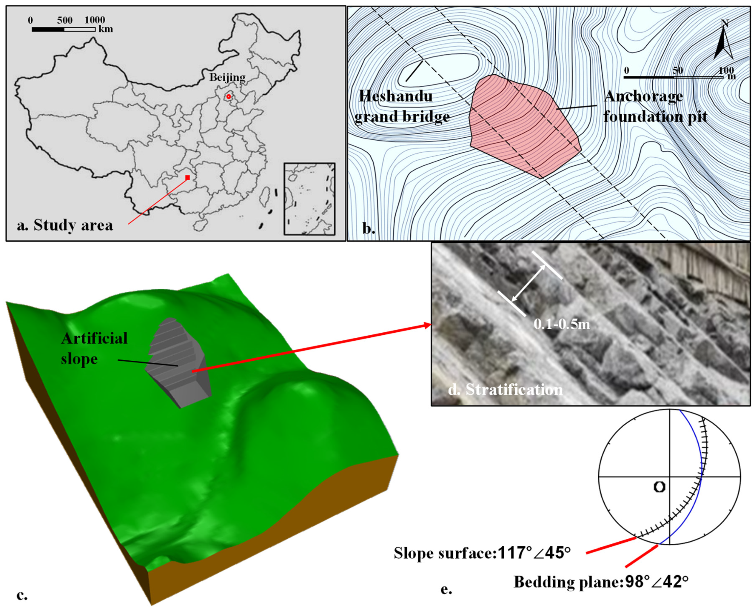
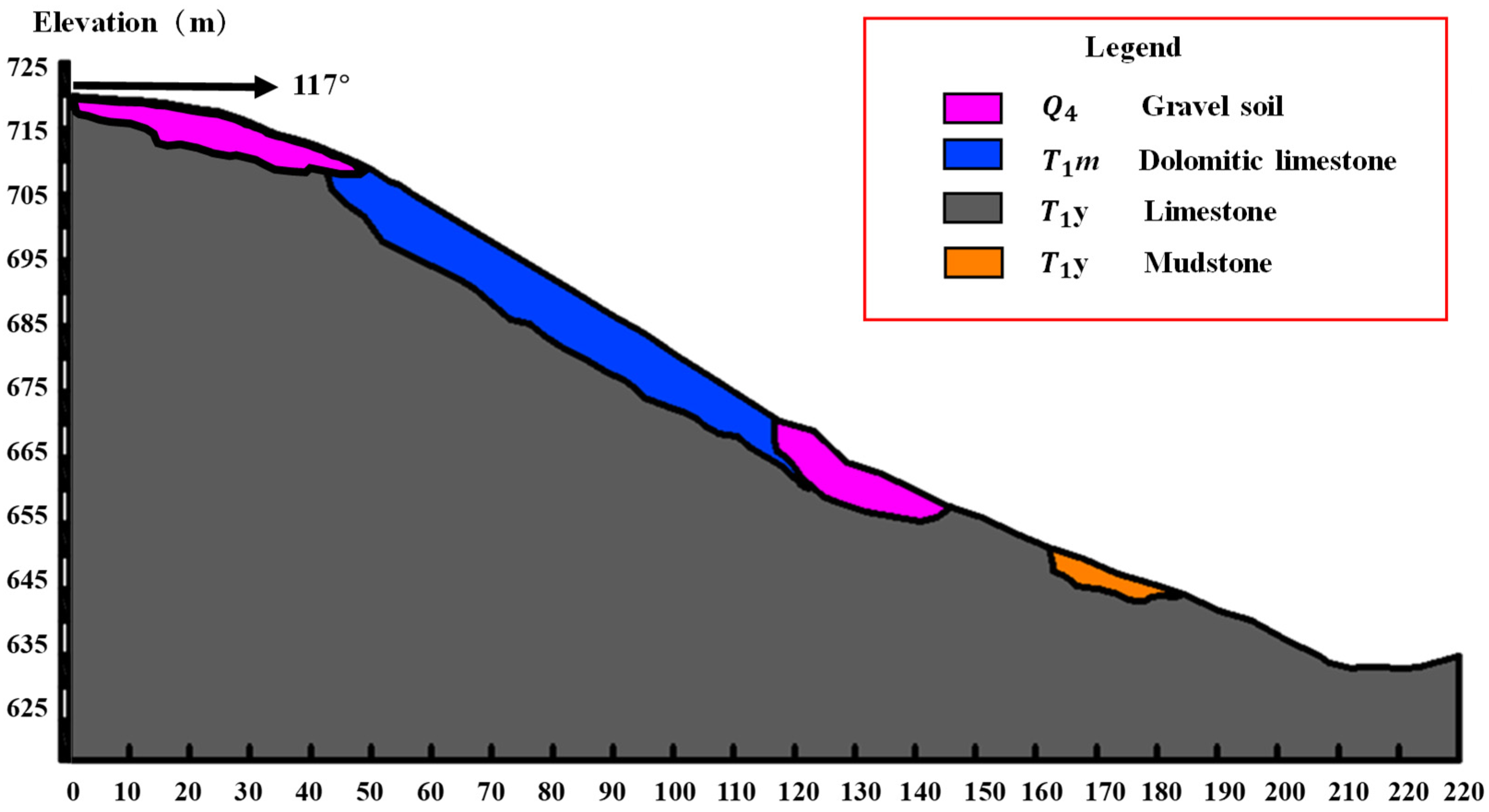
2.1. Geological Setting, Climate and Earthquake

The Wujiang River Heshandu grand bridge of the Meishi highway construction project is located in Zunyi City, Guizhou Province, China (Figure 1a). The study area is a bank slope located on the side of the Meitan. The slope is an artificial slope formed by the excavation of the anchorage foundation pit of the bridge (Figure 1b,c). The occurrence of the slope is 117°∠45°. During construction, continuous tensile cracks were observed at the back edge of the slope top. These cracks had a width ranging from 5 cm to 20 cm and a visible depth of 0.4 m. Field monitoring showed displacements exceeding the standard norms, necessitating a reassessment of safety. Detailed geological investigations and drilling were conducted to identify the lithology. Highly to moderately weathered limestone is blocky, smooth, and undulating. The bedding and joint surfaces contain no infilling. Limestone layers are arranged in a monocline. The strata outcrops belong to the Yelang (T₁y) formation of the Lower Triassic and Quaternary (Q₄), as shown in Figure 2. The mean of the limestone layer dip direction is 98° with a 2° standard deviation. The mean of the limestone layer dip is 42° with a 3.4° standard deviation. The thickness of layer is 0.1–0.5 m (Figure 1d.). The core monitor rate is 80–85%; RQD = 60–85. Two joints were found on the site, J1 188°∠48° and J2 145°∠54°.

The location belongs to an eastern subtropics monsoon climate region. The annual average temperature is 15.2 ° C. The average annual rainfall in the area is 1093 mm, mainly concentrated from May to September, and the maximum daily rainfall is 141.4 mm. The groundwater is in the range of 12.1 m to 59.1 m.

The reference area is located in an earthquake belt. Up to December 2020, 119 earthquakes with a magnitude of 4.7 or higher were recorded in this earthquake zone. All these earthquakes were shallow, including four with a magnitude of 6.09 and 66 with a magnitude of 5.09.

2.2. Engineering Overview

The bottom of the pit is a rectangle 47 m × 65 m (Figure 3a). The rear slope of the foundation pit is a bedding rock slope. The highest elevation is 720.1 m. The dip direction of the artificial slope is 117°, the elevation of the pit crest is 704.854 m, and the elevation of the toe is 625.288 m. The pit depth is 79.566 m and consists of 10 benches, as shown in profile (Figure 3b). The benches are laterally anchored by two kinds of anchor cables with a specified inclination of 30° (refer to Figure 3b and

Table 1. Information of anchors.

Locations (Step)	Number	Spacing (m)	Length (m)
1th	6	4.5	34.3
2nd	15	4.5	34.3
3rd	21	4.5	34.3
4th	26	4.5	34.3
5th	32	4.5	30.3
6th	39	4.5	30.3
7th	35	4.5	30.3
8th	26	4.5	30.3
9th	24	4.5	26.3
10th	60	2	5

for more anchor space information).

3. Methodology

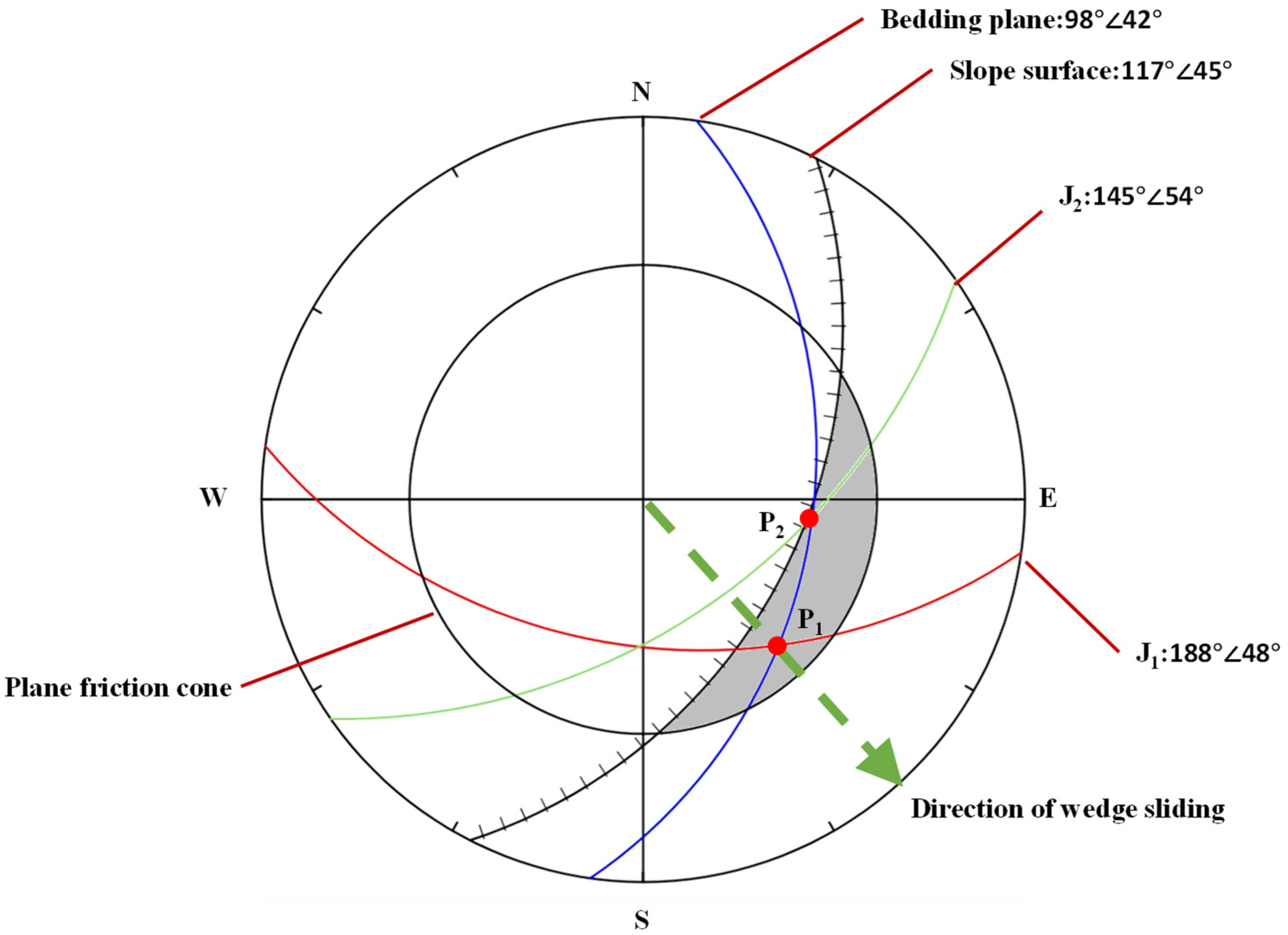
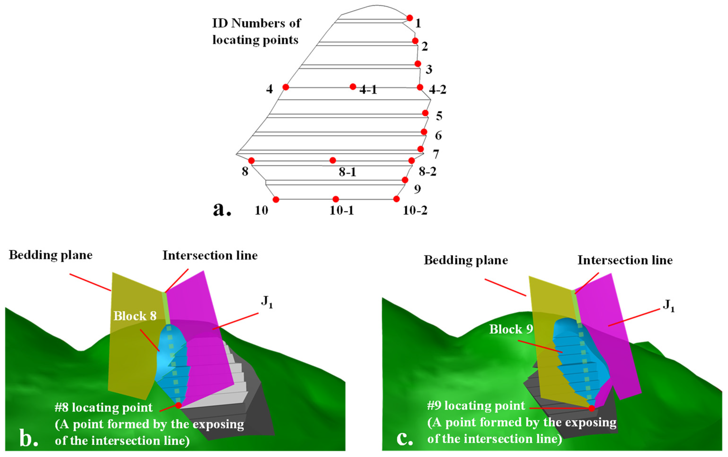
3.1. Detection of Potential Sliding Surface

The occurrence of the slope and bedding plane is 117°∠45° and 98°∠42°. Studies show wedge failure is prone to occur when the slope dip is greater than the weak structure plane dip [40]. This problem needs three-dimensional limit equilibrium analysis to determine the most dangerous plane.

Kinematic analysis (Figure 4) was utilized to determine the potential sliding line and identify two intersections (P1 and P2) of joints and bedding. The friction angles of the joint and bedding plane are 22° and 27°. The average friction angle (24.5°) of the two slide planes (joint and bedding) is expressed as a plane friction cone in Figure 4. In general, sliding may occur if the intersection point between the two great circles of the sliding planes lies within the shaded area in Figure 4. In this study, the most likely direction of wedge sliding is the orientation represented by P1.

The point where the intersection line is exposed (Figure 5b,c) can be used to locate the two sliding surfaces. We identified 16 potential blocks based on these locating points (see Figure 5a). Figure 5b,c shows two examples of the potential blocks (Block 8 and Block 9). The safety of unstable blocks was assessed using the LEM, and the results (see Section 4.1) indicated two unstable blocks (Block 8 and Block 9). Each block was then modeled in the numerical simulations (Model 1 is for Block 8, and Model 2 is for Block 9).

3.2. Numerical Evaluation

3.2.1. Constitutive Model and Material Parameters

The built-in Mohr–Coulomb Model in FLAC3D was applied for the rock constitutive models. The failure envelope for this model corresponds to a Mohr–Coulomb criterion (shear yield function) with tension cutoff (tension yield function). The position of a stress point on this envelope is controlled by a non-associated flow rule for shear failure and an associated rule for tension failure [41]. For the bedding plane, three methods are described in detail in Section 3.2.3, which contains a changing constitutive model and two improved modeling methods.

The triaxial shear tests and Brazilian tests were used to detect the shear strength (C and φ) and tensile strength of intact rock specimens. The method based on the Generalized Hoek–Brown criterion [42] was employed to estimate the intact rock modulus ($E_i$) and shear strength (C and φ) and the tensile strength and modulus ($E_r$) of the rock mass. First, we estimated the modulus ratio (MR) according to the lithology and calculated the $E_i$. Second, we estimated the Hoe–Brown constant (m_i), Geological Strength Index (GSI), and disturbance factor (D) from experiential charts. The estimations of the above four are MR = 700, m_i = 6, GSI = 55, and D = 1. Finally, these estimations were substituted in a series of empirical equations [42] to determine the C, φ, tensile strength, and $E_r$ of the rock mass. For the shear strength of the bedding plane, we adopted estimations recommended by national standards. Lastly, we extracted the mechanical properties of the anchorage structure from the engineering report.

Table 2. Mechanical properties of rock.

Material Properties	Density (kN/m3)	Cohesion C (MPa)	Internal Friction Angle φ (°)	Uniaxial Compressive Strengths		Modulus		Tensile Strength (MPa)
				${\mathit{\sigma }}_{\mathit{c}\mathit{i}}$ (MPa)	${\mathit{\sigma }}_{\mathit{c}}$ (MPa)	${\mathit{E}}_{\mathit{i}}$ (GPa)	${\mathit{E}}_{\mathit{r}}$ (GPa)
Intact rock	27	14.7	31.3	63	——	44.1	——	5.9
Rock mass	24.7	0.5	30.7	——	1.4	——	4.0	0.14
Bedding plane	27	0.09	27	——	——	——	——	——

and

Table 3. Mechanical properties of anchorage structure.

Types of Anchorage	Cross-Sectional Area (m2)	Young’s Modulus (GPa)	Tensile Yield Strength (kN)	Grout Cohesive Strength (kN)	Grout Stiffness (MPa)	Grout Exposed Perimeter (m)	Pre-Tension (kN)	Inclination (°)	Anchoring Length (m)
1	5.8 × 10−5	20	1260	1000	20	0.2512	1050	30	10.3
2	5.8 × 10−5	20	1620	1000	20	0.1884	1350	30	10.3
Cables	1 × 10−4	20	1620	1000	20	0.2512	——	30	5

summarize all the mechanical parameters.

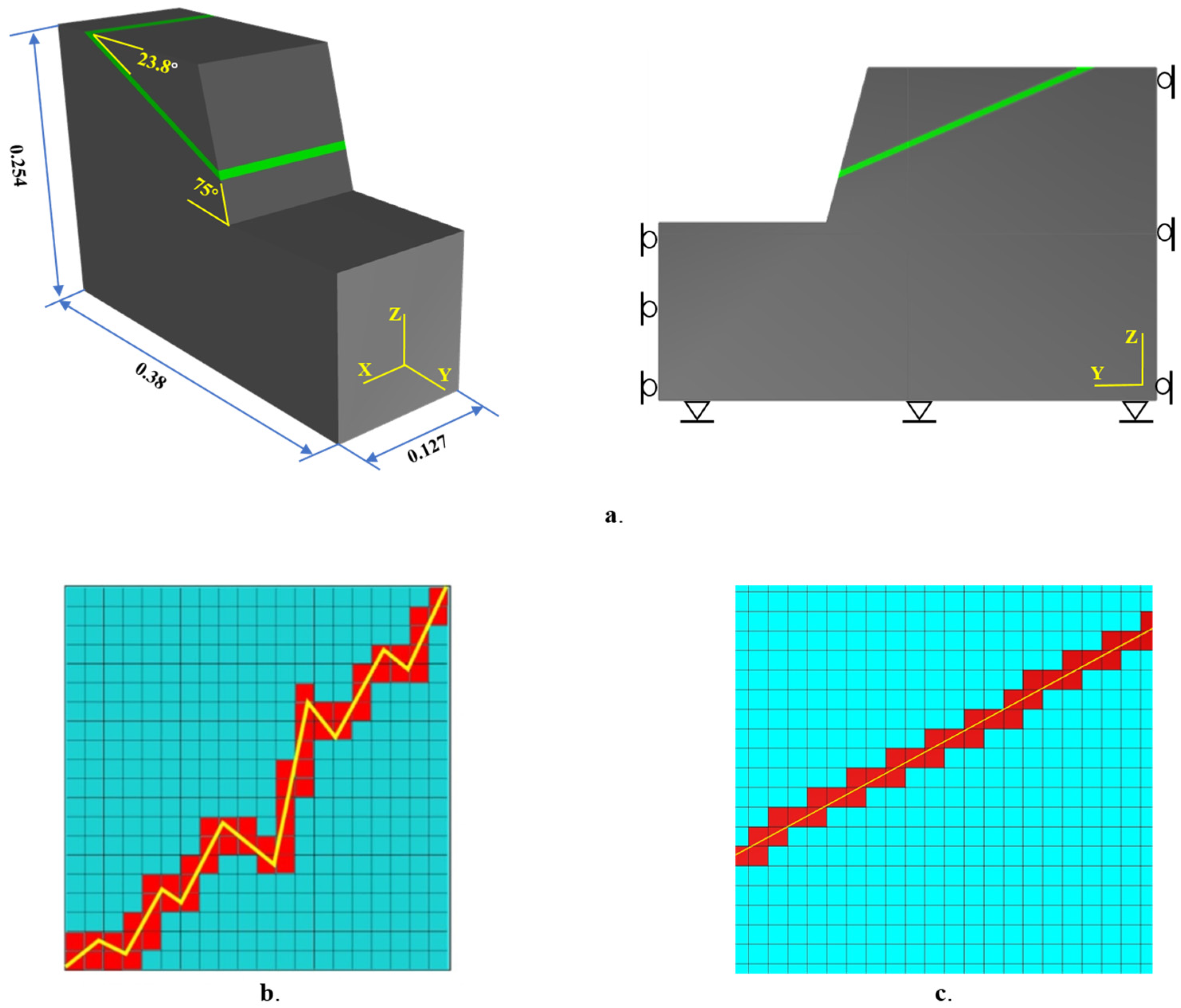
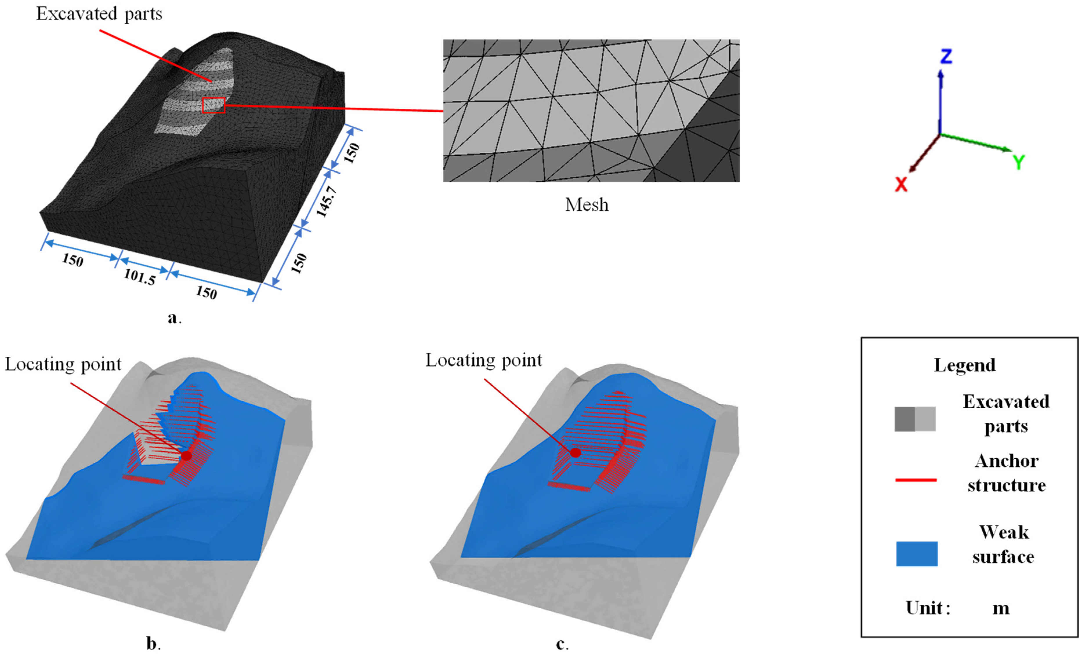
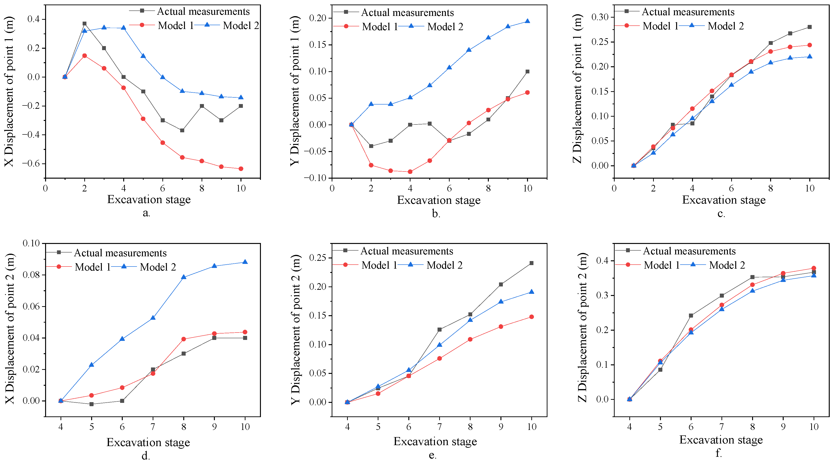
3.2.2. Model Assumptions, Mesh Generation, Boundary Conditions, and Validation

Before modeling, we validated the numerical method in this study by reproducing a the results from a study. Please refer to Appendix A.

Some assumptions were made for model operation:

• The pit is excavated in layers.
• Anchor construction and the prestressing are completed instantly with no loss of prestress.
• The anchors are considered by cable elements in the numerical model. Each cable element is defined by its geometric, material, and grout properties. The cable behaves as an elastic, perfectly plastic material that can yield in tension and compression but cannot resist a bending moment. A cable is grouted such that force develops along its length in response to relative motion between the cable and the grid. The grout behaves as an elastic, perfectly plastic material, with its peak strength being confining stress dependent and with no loss of strength after failure.

First, a pyramid-dominant mesh was generated with a specified min angle (15°) and min edge length (3 m). In this mesh, each boundary extended 150 m (Figure 6a), while the bottom extended 80 m. For the boundary conditions, horizontal motion (X and Y directions) is constrained at the four vertical boundaries, while both horizontal and vertical motions (X, Y and Z directions) are constrained at the bottom boundary. Then, the bedding planes forming two unstable blocks (Section 4.1) were inserted into the mesh and generated two models (Figure 6b is Model 1 for Block 8, and Figure 6c is Model 2 for Block 9). The mesh numbers of the two models are 33,312 (Model 1) and 34,877 (Model 2). Finally, we zoned excavated parts on the original terrain in each model (Figure 6a).

Before the model operation, the excavation was simulated to obtain the initial stress field. The excavation was simulated by a layered removal of the excavated parts and a layered setting of the anchors under gravity load. During the excavation, the deformation was monitored and compared with in situ measurements to validate the models (see Section 4.2.1).

3.2.3. Numerical Evaluation of the Slope Stability

In the present study, FOS was used to investigate the influence of different factors on slope stability. The method used to model the weak interlayers significantly influenced the slope stability analysis, and the most widely used were Weak Zone (WZ) [43,44,45], Ubiquitous-Joint (UJ) [46,47,48], and Interface (IF) [14,49]. In a recent study [50], Azarfar et al. validated each method and compared the sensitivity of each method to modeling parameters. Their study revealed that the method used to model weak interlayers (WZ, UJ, and IF) significantly influenced the slope stability analysis. It is still challenging to determine the most suitable modeling method, so the study conducted numerical evaluations using all these methods:

• The WZ method considers the weak interlayer as a ‘weak zone’ with isotropic materials and employs the Mohr–Coulomb Model [41] for modeling weak interlayers. This method treats potential sliding surfaces as isotropic materials with lower mechanical parameters in all directions, making them more conservative than other methods.
• The UJ method regards the weak interlayer as a ‘weak zone’ with anisotropic materials and uses the built-in Ubiquitous-joint constitutive model for modeling weak interlayers. This model accounts for the presence of an orientation of weakness (weak plane) in a Mohr–Coulomb model. The criterion for failure on the plane, whose orientation is given, consists of a composite Mohr–Coulomb envelope with tension cutoff. The position of a stress point on the latter envelope is controlled again by a non-associated flow rule for shear failure and an associated rule for tension failure [41]. This method maintains anisotropy, with lower mechanical properties along the bedding plane and consistent properties with other rock masses in other directions.
• The IF method considers the potential sliding surface as a two-dimensional plane unit and takes into account properties such as friction angle and cohesion. This approach does not involve the concept of interface thickness, making it closer to real-world conditions. However, the values for shear stiffness and normal stiffness of the interface need to be determined artificially. These two parameters were estimated using the recommended method in the FLAC3D manual [41]:

$$k_n={\displaystyle \frac{E{E}_r}{s(E_r-E)}}$$

(1)

$$k_S={\displaystyle \frac{G{G}_r}{s(G_r-G)}}$$

(2)

$$G_r={\displaystyle \frac{G_r}{2(1+{\mu }_r)}}$$

(3)

$$G={\displaystyle \frac{E}{2(1+\mu )}}$$

(4)

where k_n is the normal stiffness, k_s is the shear stiffness, s is the joint spacing (s = 0.5 m), E_r is the Young’s modulus of the intact rock, E is the Young’s modulus of the rock mass, G_r is the shear modulus of the intact rock, G is the shear modulus of the rock mass, μ_r is the Poisson’s ratio of the intact rock, μ is the Poisson’s ratio of the rock mass (μ_r = μ = 0.3). This estimation method requires Young’s modulus and shear modulus of the rock mass. However, Young’s modulus of the rock mass is difficult to determine in practical applications. It is assumed that Young’s modulus of the rock mass is consistent with the bedding plane. Although this consideration lacks experimental verification, it is conservative. The normal stiffness K_n and shear stiffness K_s of the interface are 1.09 × 10¹⁰ Pa/m (K_n) and 4.23 × 10⁹ Pa/m (K_s) in the present study.

3.2.4. Factors Inducing Slope Instability

The inverse analyses are focused on single-factor effects. Previous research has shown the main triggers for landslides are rainfall infiltration [51,52,53] and earthquakes [54,55,56]. Additionally, when engineering slopes are reinforced with anchorage materials, the stability changes as the anchorage force evolves [57,58]. Forward analysis, on the other hand, needs to consider multi-factor effects, which are more useful for engineering assessments. This study will take into account the effects of these single factors (rainfall, earthquakes, and anchorage force) and establish eight working conditions (see

Table 4. Working conditions.

Factors	W0	W1	W2	W3	W4	W5	W6	W7
Prestressing loss		√			√	√		√
Rainfall			√		√		√	√
Earthquake				√		√	√	√

).

The consideration for each factor in modeling is summarized as follow:

• Many previous studies have reported that the anchoring force attenuates [59,60,61]. Field monitoring data reported by Shi, et al. [62] show that the prestressing loss of anchorage cables can reach approximately 20% in 120 days. Furthermore, the corrosive environment also reduces the anchoring force. Prestressing loss caused by corrosion occurs after 120 days and reaches 4.3% [31]. Longer-term monitoring data show that the prestressing loss can reach 28.48% after more than ten years [59]. Together, these studies indicate that the prestressing loss occurs in phases. To simulate the prestressing loss, we set prestressing at three gradients: 80%, 75%, and 70% (

  Table 5. Gradients of material parameters.

  Gradients	Pre-Tension (kN)		Cohesion c (kPa)		Earthquake Influence Coefficients
  	Type 1	Type 2	Rock Mass	Bedding Plane
  1	892.5	1147.5	272.65	85.5	0.01
  2	735	945	243.95	76.5	0.03
  3	525	675	215.25	67.5	0.05

  ).
• The weakening effects caused by the interaction of water and rock will decrease the stability of a rock slope. The pore pressure will increase, and the strength will decrease under this effect. The weakening effect caused by rainfall does not include the pore pressure increasing in the present study, considering the additional complexity and computational cost involved. To better understand the mechanisms of softening, Xiong, et al. [63] analyzed the triaxial shear test data of 30 groups of dry and saturated rocks. They proposed the cohesion (C) of the saturated sample is reduced by 31.8%, and the friction angle (φ) is almost unchanged. In the present study, we set C to three gradients, as 90%, 80%, and 70%, to simulate the softening of rock materials at different saturations, listed in Table 5.
• The pseudo-static approach is a common method to analyze the slope stability subject to seismic disturbance [64]. This method simplified the problem by treating the earthquake load as a static load:

$$F=kW$$

(5)

where F is the earthquake load, W is the gravity of the sliding mass, and k is a seismic coefficient representing the size of the effect induced by the earthquake. The seismic coefficient of the study area is 0.5 g. The present study set earthquake influence coefficient gradients to reflect the slope response to different intensities (Table 5).

After modeling the weak interlayers and setting the parameters, we used a built-in strength reduction method (SRM) to compute the FOS.

3.3. Identification of Triggering Factor

Most research on the triggering factors of slope failure were based on specific slip events [65,66,67]. These post-disaster studies explained the initiation mechanism of various failure modes. Identifying the triggering factors of the failure mode before the disaster occurs is more instructive for engineering slopes. However, the exploration of this issue is not enough. Statistical methods have achieved very good application effects in the field of disaster sensitivity analysis [39,68,69,70]. These studies emphasize the statistical characteristics of data and provide a novel perspective for investigating the influence of multi-factors on slope stability. Thus, this study attempts to apply statistical methods to identify triggering factors.

Exploratory factor analysis (EFA) is a kind of multivariate statistical analysis method. EFA assumes that the correlations among variables (e.g., correlations among FOS under different working conditions) can be represented by a subset of hidden common factors [71]. Therefore, EFA is primarily used to reduce the dimension of variables by linearly combining the variables. However, the common factor cannot account for all the variations of each variable [72]. Therefore, each variable has a proportion of unique variations. Any variable can be described as a linear combination of the common factors and the unique variations [73,74]:

$$W_i=a_1{F}_1+\cdots +a_n{F}_n+U_i$$

(6)

where W_i is the ith given factor, F₁–F_n are n common factors, a₁–a_n are factor loadings (correlation coefficient between a common factor and a variable), and U_i is the unique variation of W_i. The contribution rate of variation described by a common factor represents the significance of this common factor. The factor loading measures the significance of a variable when using this variable to characterize a specific factor [70]. Most importantly, it allows one to determine how well the variable aligns with common factors and allows the identification of the most important variable according to the factor loading [75]. The commonality of a variable is the percentage of variations of this variable explained by all common factors. A commonality of a variable closer to 1 indicates a better explanation [70]. It should be noted that before the EFA analysis, the Kaiser–Meyer–Olkin (KMO) and Bartlett test of sphericity need to be implemented on the raw data to verify its feasibility [76].

First, the FOS data for each model underwent the KMO test and Bartlett test of sphericity. Next, we quantified the common factors using a scree plot to identify the number of common factors by observing the elbow point [75,77]. We then used the principal component extraction method to obtain common factors [71]. To aid interpretation, we employed varimax rotation to regenerate the common factors [78]. Finally, we determined the triggering factors of each model by comparing the factor load values. The flow chart of the EFA is shown in Figure 7.

4. Results

4.1. Results of LEM

Initially, the FOS for all blocks was calculated using the LEM. The FOS for blocks 10-2, 4-2, 3, 2, and 1 exceeded 20, while the FOS for blocks 7, 6, and 5 fell within the range of 6–10. These hypotheses need to be ruled out because the FOS values are too high. The reasons for these results will be discussed in Section 5.1. The results for the other blocks are presented in

Table 6. FOS of LEM.

Blocks	4-1	4	8	8-1	8-2	9	10	10-1
FOS	3.78	1.98	1.25	2.38	2.58	1.28	1.56	2.10

. Blocks 8 and 9 are the most unstable and are illustrated in Figure 8a. The potential sliding surfaces of the slope are represented by these two blocks, and each of them was modeled for numerical simulation (Model 1 is for Block 8, and Model 2 is for Block 9).

4.2. Results of Numerical Simulation

4.2.1. Deformation Characteristics and Sliding Modes of Slope

During the excavation stage, we monitored the deformation of the top of the slope and the fourth step, as shown in Figure 8c. We created models for the two most unstable blocks (Model 1 for Block 8 and Model 2 for Block 9) and compared the deformation data of each monitoring point with the actual field measurements (Figure 9). While it is difficult to achieve a perfect match between simulated and actual measurements, we found that the measurements are consistent in scale, and the simulated deformation aligns with the direction of the actual measurements. Both Model 1 (for Block 8—Figure 8a) and Model 2 (for Block 9—Figure 8b) reflect the deformation trend of each monitoring point. Furthermore, both models show tensile plastic zones on the top of the slope and near the cracks, as observed in situ (Section 2.1). After failure, these tensile plastic zones dilate and connect to form a crack (Figure 10a,b), indicating that both models accurately reproduce the cracks observed in situ. The results of deformation measurements and the occurrence of on-site cracks validate both models.

Figure 10 shows the failure characteristics of each model and reveals the difference in deformation features between the two models:

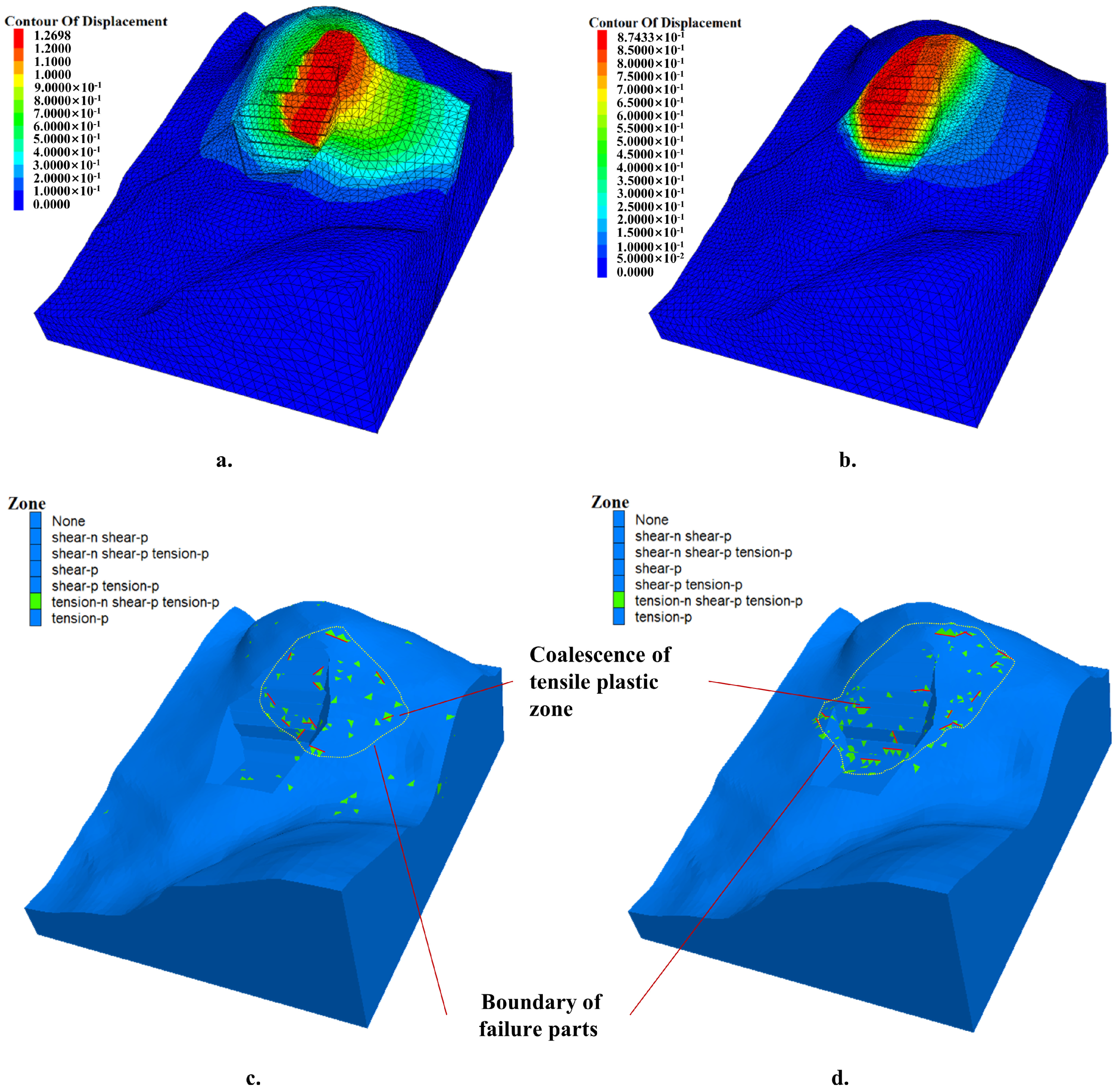
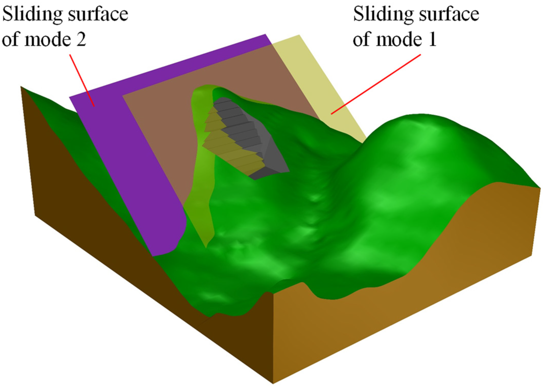
• The sliding surface of Model 1 is exposed on the slope surface (Figure 10a). The unexcavated part on the right is significantly deformed, which means the sliding block is pulling the unexcavated part of the rock mass. The coalescence of the plastic tensile zone appears on the 3rd, 5th, 7th and 8th steps (Figure 10c).
• The most significant deformation area of Model 2 is at the left (Figure 10b). The scope of the failure parts is shown in Figure 10d. The tensile plastic zone appears on the slope surface after failure and is distributed in a wider range than Model 1.

To compare the failure areas of the two models, the maximum shear strain increment of the sliding surface after failure was analyzed in Figure 11:

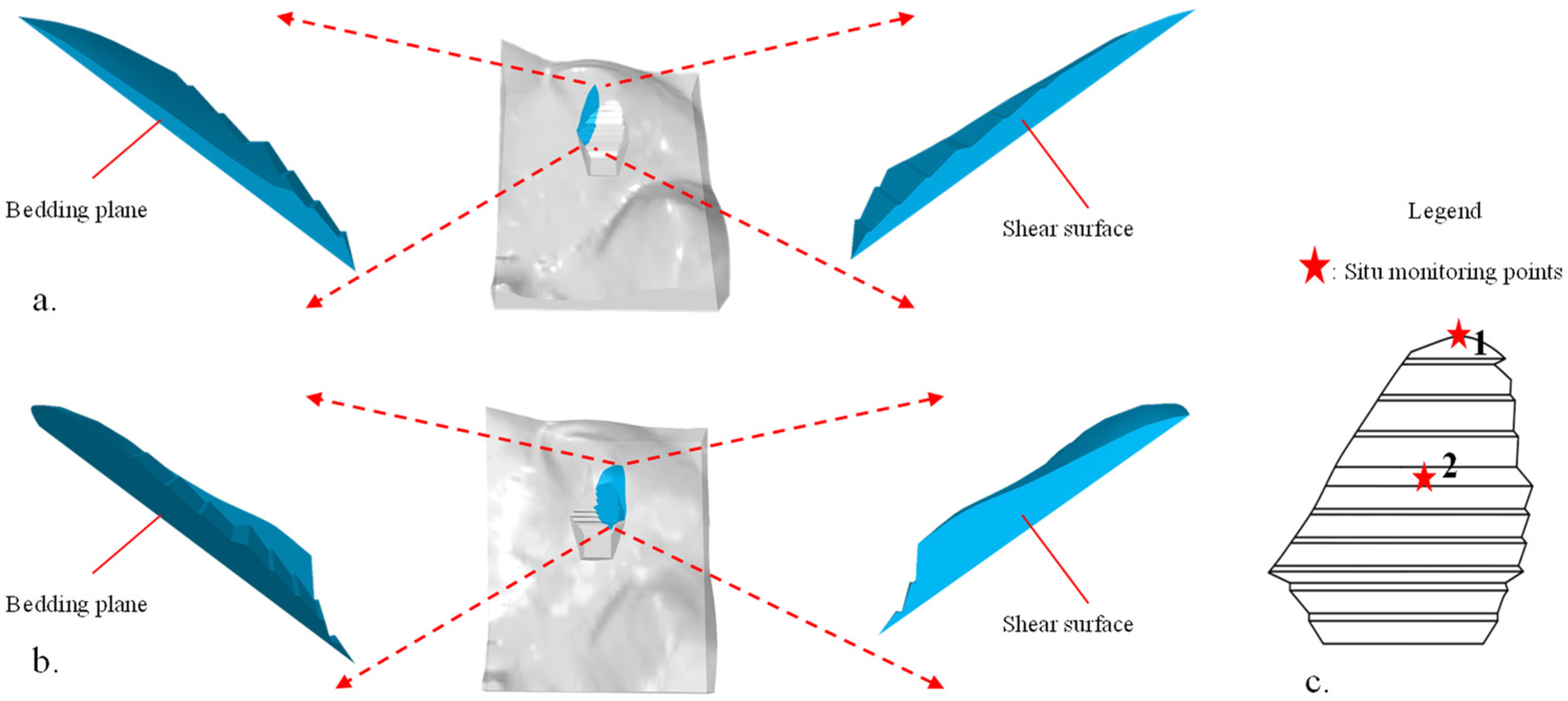
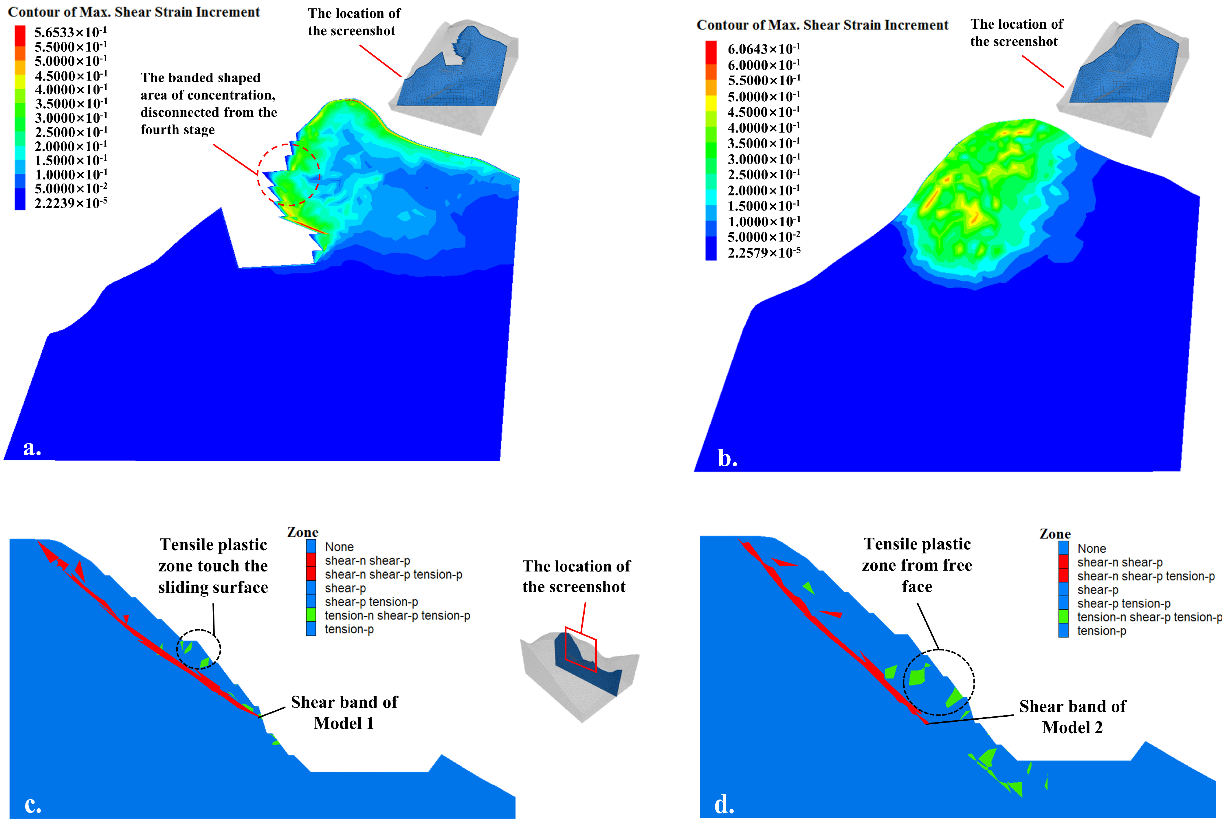
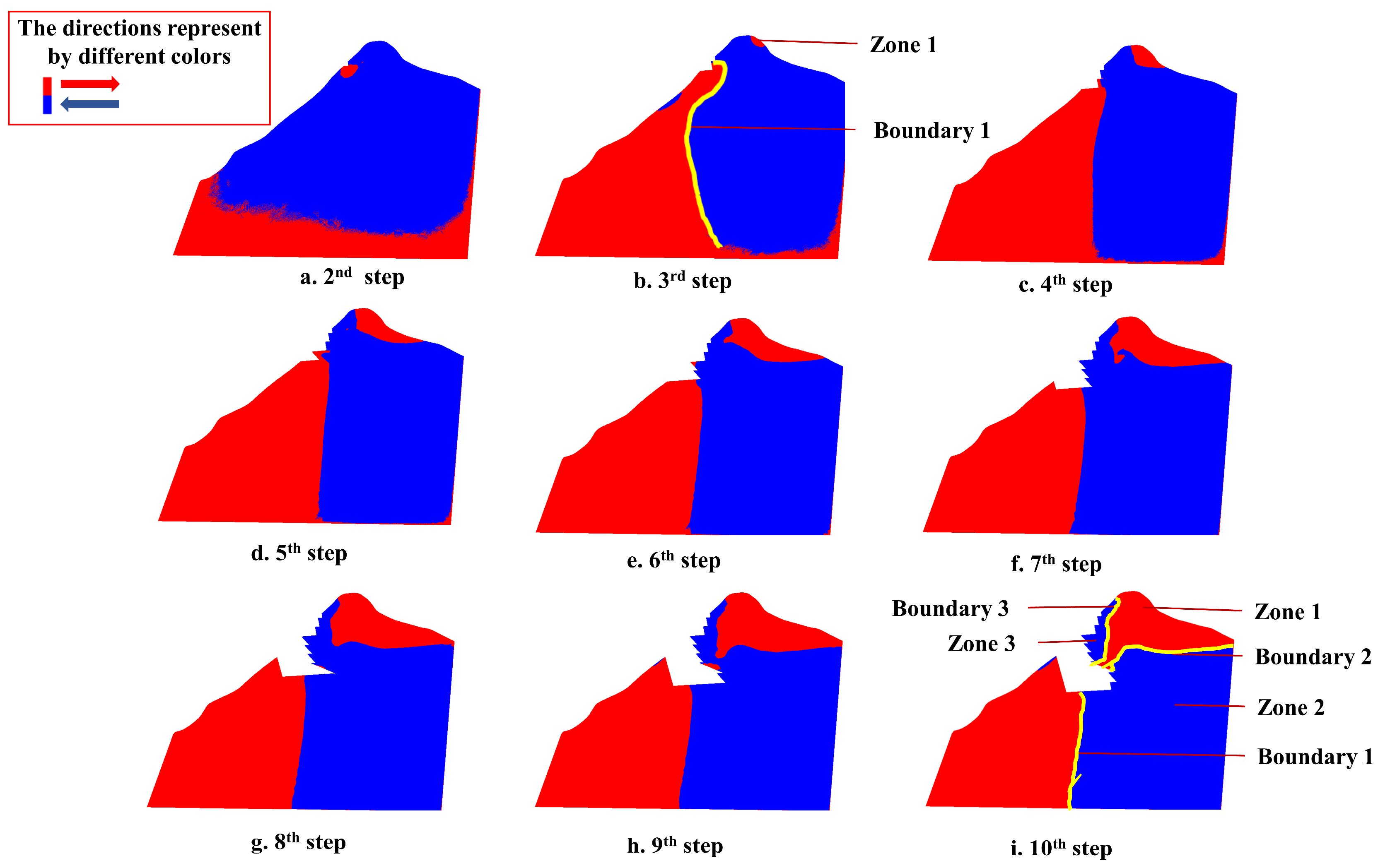
• The maximum shear strain increment is concentrated at the lower and top of the sliding surface, creating a banded concentration area in Model 1 (refer to Figure 11a). This area is very close to the daylight of the potential sliding surface. The shear strain increment area gradually diffuses to the right, indicating that the rocks in the concentrated area exert a strong drawing effect on the unexcavated rock mass. The drawing effect caused by the banded area of the sliding surface can easily lead to slope cracking and the formation of a sliding block. The forming process of this band will be discussed in Section 5.2. The sliding block may deform asymmetrically, potentially leading to rotational failure on the plane. The sliding surface of Model 1 is exposed on the slope surface, forming a sliding block. This failure mode reflects cracking from the back edge, as reported by Zhao, L.H [4].
• In Model 2 (Figure 11b), the maximum shear strain increment is concentrated at the middle and top of the slope and diminishes at the lower part. This indicates that the deformation of the entire potential sliding surface is impeded at the bottom. The bottom of the slope strongly constrains the sliding body. When the upper rock experiences significant pressure, the sliding body is susceptible to buckling failure in the middle. Even slight deformation in the middle of the sliding body can result in a substantial bending moment. Lin et al. [2] suggested that this locking phenomenon may be caused by the front edge of the slope.

The newly formed shear bands occur in the slope. The tensile plastic zones of Model 1 appear on the free face of the slope (Figure 11c.). The lower sliding body’s traction may cut off the sliding body. The tensile plastic zones of Model 2 appear between the 5th and 8th steps and are near the free face (Figure 11d). The rock mass bulging may cause bending and cracks.

4.2.2. FOS by Numerical Simulation

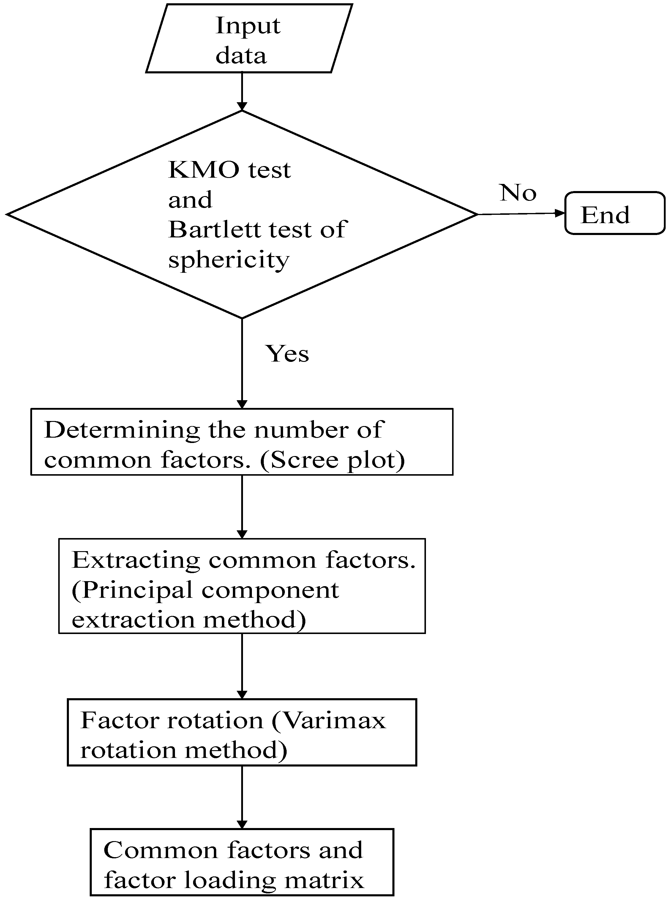
FOS calculated by SRM is shown in

Table 7. FOS of Model 1.

Methods and Gradients		W0	W1	W2	W3	W4	W5	W6	W7
WZ	G1	1.719	1.708	1.484	1.658	1.462	1.624	1.350	1.316
	G2		1.697	1.439	1.624	1.417	1.596	1.316	1.288
	G3		1.680 (2.28%)	1.383 (19.54%)	1.590 (7.49%)	1.372 (20.20%)	1.579 (8.14%)	1.277 (25.73%)	1.271 (26.06%)
UJ	G1	1.820	1.818	1.574	1.742	1.546	1.708	1.428	1.389
	G2		1.814	1.529	1.702	1.501	1.680	1.389	1.361
	G3		1.809 (0.65%)	1.467 (19.38%)	1.669 (8.31%)	1.456 (20.00%)	1.663 (8.62%)	1.350 (25.85%)	1.344 (26.15%)
IF	G1	1.865	1.863	1.652	1.764	1.630	1.730	1.473	1.434
	G2		1.862	1.607	1.725	1.585	1.702	1.434	1.406
	G3		1.859 (0.30%)	1.540 (17.42%)	1.691 (9.31%)	1.540 (17.42%)	1.686 (9.61%)	1.394 (25.23%)	1.389 (25.23%)

and

Table 8. FOS of Model 2.

Methods and Gradients		W0	W1	W2	W3	W4	W5	W6	W7
WZ	G1	1.694	1.687	1.435	1.652	1.400	1.617	1.386	1.358
	G2		1.680	1.407	1.610	1.386	1.582	1.323	1.302
	G3		1.673 (1.24%)	1.379 (18.60%)	1.561 (7.85%)	1.365 (19.42%)	1.540 (9.09%)	1.274 (24.79%)	1.253 (26.03%)
UJ	G1	1.799	1.792	1.533	1.764	1.484	1.743	1.470	1.449
	G2		1.785	1.498	1.722	1.470	1.701	1.400	1.386
	G3		1.778 (1.17%)	1.470 (18.29%)	1.666 (7.39%)	1.449 (19.46%)	1.659 (7.78%)	1.351 (24.90%)	1.337 (25.68%)
IF	G1	2.429	2.436	2.093	2.303	2.044	2.247	1.974	1.946
	G2		2.422	2.044	2.247	2.023	2.205	1.876	1.869
	G3		2.415 (0.58%)	2.009 (17.29%)	2.177 (10.37%)	1.995 (17.87%)	2.170 (10.66%)	1.813 (25.36%)	1.806 (25.65%)

(the percentage of FOS decreased from W0 is marked in the brackets). The FOS of the two models shows a very consistent trend. When the slope is individually affected by three basic factors (W1–W3), the drop of the FOS is in the range of 0.30–19.54% (Model 1, Table 7) and 0.58–18.60% (Model 2, Table 8). When subjected to double factors (W4–W6), the scope of the FOS decrease is 8.14–25.85% (Model 1, Table 7) and 7.78–25.36% (Model 2, Table 8). When all factors appear (W7), the FOS decreases in the range of 25.23–26.15% (Model 1, Table 7) and 25.65–26.03% (Model 2, Table 8).

Section 4.2.1 shows sliding surfaces in different positions lead to slope failure in two modes. The results of this section indicate the FOS has a consistent variation trend, which is an unexpected outcome. Therefore, EFA is introduced in the next section to analyze the features of the FOS data further.

4.3. EFA Results

We performed an EFA analysis on the FOS data (Table 7 and Table 8). First, the KMO test results of the two models (0.586 for Model 1 and 0.745 for Model 2) are greater than 0.5, which means the data pass the KMO test. The Sig values of the two models were both less than 0.05, which means the data pass the Bartlett test of sphericity. The results of these two test showed the data are statistically feasible. The scree plots of each model are shown in Figure 12. The ‘elbow point’ of each plot is present at 2, which indicates the most suitable number of common factors for each model is 2.

In our analysis of Model 1 (

Table 9. The factor-loading matrix, commonality, and contribution ratios for Model 1 (Model 1).

Variable	F1	F2	Commonality
W1 (Prestressing loss)	0.497	0.866	0.997
W2 (Rainfall)	0.859	0.506	0.993
W3 (Earthquake)	0.818	0.553	0.975
W4 (Prestressing loss and Rainfall)	0.815	0.564	0.983
W5 (Prestressing loss and Earthquake)	0.693	0.710	0.984
W6 (Rainfall and Earthquake)	0.840	0.542	1.000
W7 (Prestressing loss and Rainfall and Earthquake)	0.716	0.695	0.996
Contribution rate (%)	57.393	41.589
Accumulative contribution (%)	57.393	98.981

), we identified two common factors, F1 and F2, from the data. The cumulative contribution rate of variance reached 98.981%, which exceeds the recommended valid result of 70% for EFA [70]. This demonstrates high efficiency, as each commonality is greater than 0.73. Given that the contribution rate of F1 is higher than that of F2, we consider the factor determined in F1 is the primary factor, while the factor in F2 is considered is the secondary. The factors of F1 and F2 were sorted based on their factor loads. Before sorting, the researchers categorized the factors as single and double.

Table 10. Sort results of F1 (Model 1).

Single Factor		Double Factor
Variable	Factor Loading	Variable	Factor Loading
W2 (Rainfall)	0.859	W6 (Rainfall and Earthquake)	0.840
W3 (Earthquake)	0.818	W4 (Prestressing loss and Rainfall)	0.815
W1 (Prestressing loss)	0.497	W5 (Prestressing loss and Earthquake)	0.693

summarizes the sorting results of F1 (Model 1). Among the single factors, W2 represents the influence of rainfall, with the highest factor load of 0.859. In the double factors, the factors containing rainfall (W4 and W6) have greater factor loads than the factor without rainfall (W5). Table 10 indicates that the primary factor of Model 1 is rainfall. Other results were sorted and analyzed in the same manner (see Appendix B,

Table A1. Sort results of F2 (Model 1).

Single Factor		Double Factor
Variable	Factor Loading	Variable	Factor Loading
W1 (Prestressing loss)	0.866	W5 (Prestressing loss and Earthquake)	0.710
W3 (Earthquake)	0.553	W4 (Prestressing loss and Rainfall)	0.564
W2 (Rainfall)	0.506	W6 (Rainfall and Earthquake)	0.542

,

Table A2. The factor-loading matrix, commonality, and contribution ratios for Model 2 (Model 2).

Variable	F1	F2	Commonality
W1 (Prestressing loss)	0.634	0.774	1.000
W2 (Rainfall)	0.692	0.722	1.000
W3 (Earthquake)	0.732	0.681	0.999
W4 (Prestressing loss and Rainfall)	0.661	0.750	1.000
W5 (Prestressing loss and Earthquake)	0.707	0.706	0.998
W6 (Rainfall and Earthquake)	0.771	0.636	0.999
W7 (Prestressing loss and Rainfall and Earthquake)	0.757	0.653	1.000
Contribution rate (%)	50.306	49.643
Accumulative contribution (%)	50.306	99.950

,

Table A3. Sort results of F1 (Model 2).

Single Factor		Double Factor
Variable	Factor Loading	Variable	Factor Loading
W3 (Earthquake)	0.732	W6 (Rainfall and Earthquake)	0.771
W2 (Rainfall)	0.692	W5 (Prestressing loss and Earthquake)	0.707
W1 (Prestressing loss)	0.634	W4 (Prestressing loss and Rainfall)	0.661

and

Table A4. Sort results of F2 (Model 2).

Single Factor		Double Factor
Variable	Factor Loading	Variable	Factor Loading
W1 (Prestressing loss)	0.774	W4 (Prestressing loss and Rainfall)	0.750
W2 (Rainfall)	0.722	W5 (Prestressing loss and Earthquake)	0.706
W3 (Earthquake)	0.681	W6 (Rainfall and Earthquake)	0.636

). Continuing the analysis, for Model 1, the primary factor is rainfall, and the secondary factor is prestress loss. For Model 2, the primary factor is earthquake loading, and the secondary factor is prestress loss.

5. Discussion

5.1. Determination of Potential Sliding Surface of Bedding Slope

The wedge failure theory requires two specific sliding surfaces at the base. These surfaces were investigated from the failed slope. For a stable slope, the directions can only be assumed according to in situ evidence. Many case studied reported sliding along the bedding [2,4]. Consequently, this study assumes the bedding plane as a sliding surface. Another sliding surface is a measured joint. Although it agrees with the mechanical argument [79], the development of fractures is influenced by multiple factors beyond mechanical assumptions. Predicting the location of joints and cracks remains challenging. Kinematic analysis only indicates a sliding orientation, and the specific sliding block needs to be identified. The current tests show that some sliding blocks have a high FOS (Section 4.1). FOS values exceeding 6 (and even reaching 20 in some cases) are unrealistic. As the position of the sliding body is hard to predict, it is necessary to consider all possibilities (Figure 5a). For example, Block 1 (Figure 5a) shows the slope will break at the pit crest and is almost impossible. However, we still consider this block in our calculations because it is difficult to predict where failure is more likely to occur.

The current numerical method for modeling fractures is immature. It is challenging to determine the scale of joints (such as depth) from on-site information. Therefore, the joint plane is only set in the calculation model of the LEM (as shown in Figure 5 and Figure 8) and not in the numerical model.

5.2. Failure Modes

The deformation of the sliding surface in Model 1 during the excavation needs to be discussed further. Figure 13 displays a map of the y-direction displacement during the excavation, with the red area representing right displacement and the blue area representing left displacement.

The shape of the potential sliding surface changed at the beginning of the second excavation (Figure 13a). The y-direction displacement of the rock mass below the new outcrop also changed. When the third step was excavated, Boundary 1 was formed (Figure 13b), causing the rock mass on both sides to squeeze. This reflects the release of elastic deformation energy in the deep rock mass. Boundary 1 tends to become stable as the excavation continues. Zone 1 is developing towards the new exposed line of the potential sliding surface (Figure 13b–i). Zone 1 divided the rock mass into three parts when the excavation was finished (Figure 13i). A shear dislocation occurs between Zone 1 and Zone 2 (Figure 13i), forming a shear boundary as Boundary 2. Additionally, a banded area in Zone 3 is formed by the tension Boundary 3. This process explains the formation of the banded-shaped area.

The displacement cloud map in Figure 14 shows the Y-direction movement of the sliding surface after failure. Boundary 2 runs through the sliding surface, dividing the original Zone 3 (Figure 13i) into upper and lower parts. This suggests that the rock mass of the fourth step experienced relative displacement and may result in a crack. Eventually, Boundary 3 is likely to develop a pull crack on the right side of the excavated slope, indicating a tendency for the right boundary of the sliding body to crack during failure. Boundary 1 disappears as elastic deformation energy is released after failure.

5.3. Exploratory Factor Analysis

In this section, we will explore the feasibility of using EFA and the engineering significance of the results obtained from EFA.

When it comes to measuring raw data, there are traditionally four levels: nominal, ordinal, interval, and ratio. Ratio data is measured in equal distances with an “absolute zero point”. It is important to note that analyzing the other three types of data with EFA may have some conceptual limitations, except for ratio data [67]. In theory, EFA is most suitable for analyzing ratio data, such as FOS. In the field of geotechnical engineering, FOS is used to measure slope stability, where a FOS < 1 indicates that the slope is unstable. The number ‘1’ represents the ‘absolute zero point’ of stability in slope engineering. Therefore, FOS data fall into the ratio category, making it feasible to use EFA for FOS data analysis.

The slope can fail in different ways, as outlined in Section 4.2.1. The researchers used three types of weak interlayer simulation methods in the FOS calculations. It is confusing that the FOS of the two failure modes show similar trends. It is hard to determine the order of variable importance directly from the FOS data. EFA provides a preferable solution to primarily elucidate the importance levels of triggering factors of different failure modes. The factor loading reflects the importance of each variable in a common factor. The more important variable has the greater factor load value. We sorted and analyzed the factor load matrix. The aim was to find the variable that has the greatest impact on each common factor.

Figure 15 compares the position of the sliding surfaces; it is clear that the sliding surface of Mode 1 is relatively shallower than that of Mode 2. That is to say, the influenced scope of Mode 1 is smaller than that of Mode 2. In fact, for a particular slope, although different conditions can induce its instability, the scope of instability depends on the destructive power of the triggering factors. Specifically, the impact of rainfall on the slope is limited, so generally, the failure scope induced by it is relatively small [80]. Unpredictable earthquakes trigger bedding rock landslides that are often characterized by large scales and fast speeds [80]. EFA detects this well in the FOS data. For Mode 1, a local failure mode, EFA identified rainfall as the main triggering factor. For Mode 2, a relatively large-scale failure mode, EFA identified earthquakes as the main triggering factor. The secondary factor of these two failure modes is prestressing loss, which shows that the anchoring structure has a non-negligible effect on slope stability. EFA explains the factors of the failure modes from a statistical point of view, and its results also reflect rationality. Bringing EFA into the process of forward analysis can help designers identify the main triggers and make decisions early. Based on the results in Section 4.2.1 and Section 4.3, we provide the following suggestions for future mitigation:

• Drainage ditches should be added at the slope to moderate the seepage caused by rainfall. The occurrence of cracks should be monitored to deal with the occurrence of local damage (Failure Mode 1).
• Measures to resist horizontal load should be set to prevent the development of deep sliding surfaces (Failure Mode 2), including, but not limited to, increasing the anchoring depth, improving the material resistance of the anchoring section, and optimizing the inclination of the anchoring structure.

6. Conclusions

This paper presents the results of a stability analysis and numerical simulation of a rock slope. It explores a statistical approach to semi-quantitatively evaluate landslide hazards in relation to potential triggers of a rock slope failure. The LEM was used to search the potential sliding surfaces, proving the possibility of multiple potential sliding surfaces of the slope. The displacement and deformation of each model were analyzed to clarify two failure modes. The range of the two failure modes and the formation mechanism of local failure modes were discussed. EFA was adopted to research the trigger factors of each failure mode. The results of the EFA were discussed from a mechanical standpoint. The introduction of EFA into the identification of triggering factors of potential failure modes has promise for future research in related fields. The following conclusions are drawn:

• According to the simulation results, the potential slope failure mechanism varies based on the specific trigger.
• EFA can productively extract the underlying information of the FOS and identify the trigger of slope failure. Bringing EFA into the process of forward analysis can help designers identify the main triggers and make decisions early.

The research method in this paper is of guiding significance for rock slope engineering which is about to be constructed or under construction. However, there are still certain limitations in this paper:

• This study only considers the reduction of rock strength parameters in rainy conditions. However, it does not take into account the additional load from water seepage, which increases internal stresses and makes the slope more susceptible to instability.
• In this paper, earthquake loading is treated as a constant horizontal force. Seismic waves generated by earthquakes propagate in all directions but can be affected by the local geological structure. Slopes closer to the earthquake’s epicenter experience stronger, more directional vibrations, and may also undergo rotations. Additionally, steep slopes are more susceptible to horizontal vibrations, which in this manuscript were considered.

References

1. Hoek, E.; Bray, J. Rock Slope Engineering, 3rd ed.; Inst. Mining and Metallurgy: London, UK, 1981; p. 358. [Google Scholar]
2. Lin, F.; Wu, L.Z.; Huang, R.Q.; Zhang, H. Formation and characteristics of the Xiaoba landslide in Fuquan, Guizhou, China. Landslides 2018, 15, 669–681. [Google Scholar] [CrossRef]
3. Zhang, S.-L.; Zhu, Z.-H.; Qi, S.-C.; Hu, Y.-X.; Du, Q.; Zhou, J.-W. Deformation process and mechanism analyses for a planar sliding in the Mayanpo massive bedding rock slope at the Xiangjiaba Hydropower Station. Landslides 2018, 15, 2061–2073. [Google Scholar] [CrossRef]
4. Zhao, L.; Li, D.; Tan, H.; Cheng, X.; Zuo, S. Characteristics of failure area and failure mechanism of a bedding rockslide in Libo County, Guizhou, China. Landslides 2019, 16, 1367–1374. [Google Scholar] [CrossRef]
5. Feng, P.; Lajtai, E.Z. Probabilistic treatment of the sliding wedge with EzSlide. Eng. Geol. 1998, 50, 153–163. [Google Scholar] [CrossRef]
6. Tofani, V.; Dapporto, S.; Vannocci, P.; Casagli, N. Infiltration, seepage and slope instability mechanisms during the 20–21 November 2000 rainstorm in Tuscany, central Italy. Nat. Hazards Earth Syst. Sci. 2006, 6, 1025–1033. [Google Scholar] [CrossRef]
7. Frayssines, M.; Hantz, D. Modelling and back-analysing failures in steep limestone cliffs. Int. J. Rock Mech. Min. 2009, 46, 1115–1123. [Google Scholar] [CrossRef]
8. Paronuzzi, P.; Rigo, E.; Bolla, A. Influence of filling-drawdown cycles of the Vajont reservoir on Mt. Toc slope stability. Geomorphology 2013, 191, 75–93. [Google Scholar] [CrossRef]
9. Eberhardt, E.; Stead, D.; Coggan, J. Numerical analysis of initiation and progressive failure in natural rock slopes—The 1991 Randa rockslide. Int. J. Rock Mech. Min. 2004, 41, 69–87. [Google Scholar] [CrossRef]
10. Sturzenegger, M.; Stead, D. The Palliser Rockslide, Canadian Rocky Mountains: Characterization and modeling of a stepped failure surface. Geomorphology 2012, 138, 145–161. [Google Scholar] [CrossRef]
11. Boon, C.; Houlsby, G.; Utili, S. New insights into the 1963 Vajont slide using 2D and 3D distinct-element method analyses. Geotechnique 2014, 64, 800–816. [Google Scholar] [CrossRef]
12. Sandøy, G.; Oppikofer, T.; Nilsen, B. Why did the 1756 Tjellefonna rockslide occur? A back-analysis of the largest historic rockslide in Norway. Geomorphology 2017, 289, 78–95. [Google Scholar] [CrossRef]
13. Chen, G.-Q.; Huang, R.-Q.; Zhang, F.-S.; Zhu, Z.-F.; Shi, Y.-C.; Wang, J.-C. Evaluation of the possible slip surface of a highly heterogeneous rock slope using dynamic reduction method. J. Mt. Sci. 2018, 15, 672–684. [Google Scholar] [CrossRef]
14. Bolla, A.; Paronuzzi, P. Numerical Investigation of the Pre-collapse Behavior and Internal Damage of an Unstable Rock Slope. Rock Mech. Rock Eng. 2020, 53, 2279–2300. [Google Scholar] [CrossRef]
15. Franci, A.; Cremonesi, M.; Perego, U.; Oñate, E.; Crosta, G. 3D simulation of Vajont disaster. Part 2: Multi-failure scenarios. Eng. Geol. 2020, 279, 105856. [Google Scholar] [CrossRef]
16. Fan, G.; Zhang, J.; Wu, J.; Yan, K. Dynamic Response and Dynamic Failure Mode of a Weak Intercalated Rock Slope Using a Shaking Table. Rock Mech. Rock Eng. 2016, 49, 3243–3256. [Google Scholar] [CrossRef]
17. Tang, H.; Yong, R.; Eldin, M.A.M.E. Stability analysis of stratified rock slopes with spatially variable strength parameters: The case of Qianjiangping landslide. Bull. Eng. Geol. Environ. 2017, 76, 839–853. [Google Scholar] [CrossRef]
18. Tang, J.; Dai, Z.; Wang, Y.; Zhang, L. Fracture Failure of Consequent Bedding Rock Slopes After Underground Mining in Mountainous Area. Rock Mech. Rock Eng. 2019, 52, 2853–2870. [Google Scholar] [CrossRef]
19. Rotaru, A.; Bejan, F.; Almohamad, D. Sustainable Slope Stability Analysis: A Critical Study on Methods. Sustainability 2022, 14, 8847. [Google Scholar] [CrossRef]
20. Steiakakis, E.; Xiroudakis, G.; Lazos, I.; Vavadakis, D.; Bazdanis, G. Stability Analysis of a Multi-Layered Slope in an Open Pit Mine. Geosciences 2023, 13, 359. [Google Scholar] [CrossRef]
21. Tang, C.A.; Liang, Z.Z.; Zhang, Y.B.; Chang, X.; Tao, X.; Wang, D.G.; Zhang, J.X.; Liu, J.S.; Zhu, W.C.; Elsworth, D. Fracture spacing in layered materials: A new explanation based on two-dimensional failure process modeling. Am. J. Sci. 2008, 308, 49–72. [Google Scholar] [CrossRef]
22. Xu, T.; Ranjith, P.; Wasantha, P.; Zhao, J.; Tang, C.; Zhu, W. Influence of the geometry of partially-spanning joints on mechanical properties of rock in uniaxial compression. Eng. Geol. 2013, 167, 134–147. [Google Scholar] [CrossRef]
23. Vergara, M.R.; Kudella, P.; Triantafyllidis, T. Large Scale Tests on Jointed and Bedded Rocks Under Multi-Stage Triaxial Compression and Direct Shear. Rock Mech. Rock Eng. 2015, 48, 75–92. [Google Scholar] [CrossRef]
24. Zhou, J.-F.; Qin, C.-B. A novel procedure for 3D slope stability analysis: Lower bound limit analysis coupled with block element method. Bull. Eng. Geol. Environ. 2020, 79, 1815–1829. [Google Scholar] [CrossRef]
25. Yan, C.; Wang, H. Three-dimensional stability of slopes with cut-fill interface based on upper-bound limit analysis. Yantu Gongcheng Xuebao/Chin. J. Geotech. Eng. 2024, 46, 174–181. [Google Scholar]
26. Van Eeckhout, E.M. The mechanisms of strength reduction due to moisture in coal mine shales. Int. J. Rock Mech. Min. Sci. Geomech. Abstr. 1976, 13, 61–67. [Google Scholar] [CrossRef]
27. Vasarhelyi, B. Some observations regarding the strength and deformability of sandstones in dry and saturated conditions. Bull. Eng. Geol. Environ. 2003, 62, 245–249. [Google Scholar] [CrossRef]
28. Li, D.; Wong, L.N.Y.; Liu, G.; Zhang, X. Influence of water content and anisotropy on the strength and deformability of low porosity meta-sedimentary rocks under triaxial compression. Eng. Geol. 2012, 126, 46–66. [Google Scholar] [CrossRef]
29. Wasantha, P.; Ranjith, P. Water-weakening behavior of Hawkesbury sandstone in brittle regime. Eng. Geol. 2014, 178, 91–101. [Google Scholar] [CrossRef]
30. Song, Y.; Li, Y. Study on the constitutive model of the whole process of macroscale and mesoscale shear damage of prestressed anchored jointed rock. Bull. Eng. Geol. Environ. 2021, 80, 6093–6106. [Google Scholar] [CrossRef]
31. Li, C.; Zhang, R.-T.; Zhu, J.-B.; Liu, Z.-J.; Lu, B.; Wang, B.; Jiang, Y.-Z.; Liu, J.-S.; Zeng, P. Model test of the stability degradation of a prestressed anchored rock slope system in a corrosive environment. J. Mt. Sci. 2020, 17, 2548–2561. [Google Scholar] [CrossRef]
32. Wu, S.G.; Fu, H.M.; Zhang, Y.Y. Study on anchorage mechanism and application of tension-compression dispersive anchor cable. Rock Soil Mechanics. 2018, 39, 2155. [Google Scholar]
33. Zheng, D.; Liu, F.-Z.; Ju, N.-P.; Frost, J.D.; Huang, R.-Q. Cyclic load testing of pre-stressed rock anchors for slope stabilization. J. Mt. Sci. 2016, 13, 126–136. [Google Scholar] [CrossRef]
34. Li, J.; Law, S.; Ding, Y. Substructure damage identification based on response reconstruction in frequency domain and model updating. Eng. Struct. 2012, 41, 270–284. [Google Scholar] [CrossRef]
35. Wang, Z.; Chen, G. Analytical mode decomposition with Hilbert transform for modal parameter identification of buildings under ambient vibration. Eng. Struct. 2014, 59, 173–184. [Google Scholar] [CrossRef]
36. Song, D.; Chen, Z.; Ke, Y.; Nie, W. Seismic response analysis of a bedding rock slope based on the time-frequency joint analysis method: A case study from the middle reach of the Jinsha River, China. Eng. Geol. 2020, 274, 105731. [Google Scholar] [CrossRef]
37. Johnson, P.A.; McCuen, R.H.; Hromadka, T.V. Magnitude and frequency of debris flows. J. Hydrol. 1991, 123, 69–82. [Google Scholar] [CrossRef]
38. Shi, M.; Chen, J.; Song, Y.; Zhang, W.; Song, S.; Zhang, X. Assessing debris flow susceptibility in Heshigten Banner, Inner Mongolia, China, using principal component analysis and an improved fuzzy C-means algorithm. Bull. Eng. Geol. Environ. 2016, 75, 909–922. [Google Scholar] [CrossRef]
39. Liang, Z.; Wang, C.; Han, S.; Khan, K.U.J.; Liu, Y. Classification and susceptibility assessment of debris flow based on a semi-quantitative method combination of the fuzzy C-means algorithm, factor analysis and efficacy coefficient. Nat. Hazards Earth Syst. Sci. 2020, 20, 1287–1304. [Google Scholar] [CrossRef]
40. Bowa, V.M.; Kasanda, T. Wedge Failure Analyses of the Jointed Rock Slope Influenced by Foliations. Geotech. Geol. Eng. 2020, 38, 4701–4710. [Google Scholar] [CrossRef]
41. Itasca. FLAC3D Fast Lagrangian Analysis of Continua in 3Dimensions User’s Guide Fifth Edition (FLAC3D Version 5.0); Itasca Consulting Group: Minneapolis, MN, USA, 2012. [Google Scholar]
42. Hoek, E. Practical Rock Engineering. 2007. Available online: https://www.rocscience.com/learning/hoeks-corner (accessed on 25 June 2024).
43. Tutluoglu, L.; Öge, I.F.; Karpuz, C. Two and three dimensional analysis of a slope failure in a lignite mine. Comput. Geosci. 2011, 37, 232–240. [Google Scholar] [CrossRef]
44. Chang, K.-T.; Ge, L.; Lin, H.-H. Slope creep behavior: Observations and simulations. Environ. Earth Sci. 2015, 73, 275–287. [Google Scholar] [CrossRef]
45. Yu, F.; Zhang, Y.; Chen, S.X.; Li, J. Numerical Simulation Study on the Failure Mechanism of Bedding Rock Slope Based on the Lagrangian Multiplier Method. In Applied Science, Materials Science and Information Technologies in Industry; Liu, D.L., Zhu, X.B., Xu, K.L., Fang, D.M., Eds.; Applied Mechanics and Materials; Trans Tech Publications Ltd.: Zurich, Switzerland, 2014; Volume 513–517, pp. 2603–2606. [Google Scholar]
46. Jiang, Q.-Q. Strength reduction method for slope based on a ubiquitous-joint criterion and its application. Min. Sci. Technol. (China) 2009, 19, 452–456. [Google Scholar] [CrossRef]
47. Wang, T.-T.; Huang, T.-H. Anisotropic Deformation of a Circular Tunnel Excavated in a Rock Mass Containing Sets of Ubiquitous Joints: Theory Analysis and Numerical Modeling. Rock Mech. Rock Eng. 2014, 47, 643–657. [Google Scholar] [CrossRef]
48. Sainsbury, B.L.; Sainsbury, D.P. Practical Use of the Ubiquitous-Joint Constitutive Model for the Simulation of Anisotropic Rock Masses. Rock Mech. Rock Eng. 2017, 50, 1507–1528. [Google Scholar] [CrossRef]
49. Zhang, K.; Cao, P.; Meng, J.; Li, K.; Fan, W. Modeling the Progressive Failure of Jointed Rock Slope Using Fracture Mechanics and the Strength Reduction Method. Rock Mech. Rock Eng. 2015, 48, 771–785. [Google Scholar] [CrossRef]
50. Azarfar, B.; Ahmadvand, S.; Sattarvand, J.; Abbasi, B. Stability Analysis of Rock Structure in Large Slopes and Open-Pit Mine: Numerical and Experimental Fault Modeling. Rock Mech. Rock Eng. 2019, 52, 4889–4905. [Google Scholar] [CrossRef]
51. Cai, F.; Ugai, K.; Wakai, A.; Li, Q. Effects of horizontal drains on slope stability under rainfall by three-dimensional finite element analysis. Comput. Geotech. 1998, 23, 255–275. [Google Scholar] [CrossRef]
52. Wilkinson, P.L.; Anderson, M.G.; Lloyd, D.M. An integrated hydrological model for rain-induced landslide prediction. Earth Surf. Process. Landf. 2002, 27, 1285–1297. [Google Scholar] [CrossRef]
53. Raj, M.; Sengupta, A. Rain-triggered slope failure of the railway embankment at Malda, India. Acta Geotech. 2014, 9, 789–798. [Google Scholar] [CrossRef]
54. Keefer, D.K. Landslides caused by earthquakes. GSA Bull. 1984, 95, 406–421. [Google Scholar] [CrossRef]
55. Evans, S.G.; Roberts, N.J.; Ischuk, A.; Delaney, K.B.; Morozova, G.S.; Tutubalina, O. Landslides triggered by the 1949 Khait earthquake, Tajikistan, and associated loss of life. Eng. Geol. 2009, 109, 195–212. [Google Scholar] [CrossRef]
56. Xu, C.; Xu, X.; Shyu, J.B.H. Database and spatial distribution of landslides triggered by the Lushan, China Mw 6.6 earthquake of 20 April 2013. Geomorphology 2015, 248, 77–92. [Google Scholar] [CrossRef]
57. Jiang, S.-H.; Li, D.-Q.; Zhang, L.M.; Zhou, C.B. Time-dependent system reliability of anchored rock slopes considering rock bolt corrosion effect. Eng. Geol. 2014, 175, 1–8. [Google Scholar] [CrossRef]
58. Divi, S.; Chandra, D.; Daemen, J. Corrosion susceptibility of potential rock bolts in aerated multi-ionic simulated concentrated water. Tunn. Undergr. Space Technol. 2011, 26, 124–129. [Google Scholar] [CrossRef]
59. Fan, Q.; Zhu, H.; Geng, J. Monitoring result analyses of high slope of five-step ship lock in the Three Gorges Project. J. Rock Mech. Geotech. Eng. 2015, 7, 199–206. [Google Scholar] [CrossRef]
60. Sung, H.-J.; Do, T.M.; Kim, J.-M.; Kim, Y.-S. Long-term monitoring of ground anchor tensile forces by FBG sensors embedded tendon. Smart Struct. Syst. 2017, 19, 269–277. [Google Scholar] [CrossRef]
61. Lu, G.R.; Wang, Q.B.; Li, X.J.; Wang, L.G. Study and Practice of Controlling Anchorage Force Loss of Prestressed Anchor Rope. Appl. Mech. Mater. 2012, 166–169, 1663–1668. [Google Scholar] [CrossRef]
62. Shi, K.; Wu, X.; Tian, Y.; Xie, X. Analysis of Re-Tensioning Time of Anchor Cable Based on New Prestress Loss Model. Mathematics 2021, 9, 1094. [Google Scholar] [CrossRef]
63. Xiong, D.; Zhao, Z.; Chengdong, S.U.; Wang, G. Experimental study of effect of water-saturated state on mechanical properties of rock in coal measure strata. Chin. J. Rock Mech. Eng. 2011, 30, 998–1006. [Google Scholar]
64. Zheng, Y.; Chen, C.; Liu, T.; Ren, Z. A new method of assessing the stability of anti-dip bedding rock slopes subjected to earthquake. Bull. Eng. Geol. Environ. 2021, 80, 3693–3710. [Google Scholar] [CrossRef]
65. Duan, Z.; Cheng, W.-C.; Peng, J.-B.; Wang, Q.-Y.; Chen, W. Investigation into the triggering mechanism of loess landslides in the south Jingyang platform, Shaanxi province. Bull. Eng. Geol. Environ. 2019, 78, 4919–4930. [Google Scholar] [CrossRef]
66. Sultan, N.; Cochonat, P.; Canals, M.; Cattaneo, A.; Dennielou, B.; Haflidason, H.; Laberg, J.; Long, D.; Mienert, J.; Trincardi, F.; et al. Triggering mechanisms of slope instability processes and sediment failures on continental margins: A geotechnical approach. Mar. Geol. 2004, 213, 291–321. [Google Scholar] [CrossRef]
67. Shen, C.; Sun, J.; Zhang, X.; Luo, Z.; Kong, J.; Lu, C. Study on the role of lateral unsaturated flow in triggering slope failure under varying boundary water level conditions. Adv. Water Resour. 2020, 143, 103669. [Google Scholar] [CrossRef]
68. Choi, Y.N.; Hwan, H.S.; Lee, H.H.; Yoo, N.J. Estimation of Magnitude of Debris Flow and Correlation Analysis Between Influencing Factors. J. Korean Geosynth. Soc. 2017, 16, 79–87. [Google Scholar]
69. Li, Z.; Chen, J.; Tan, C.; Zhou, X.; Li, Y.; Han, M. Debris flow susceptibility assessment based on topo-hydrological factors at different unit scales: A case study of Mentougou district, Beijing. Environ. Earth Sci. 2021, 80, 365. [Google Scholar] [CrossRef]
70. Reimann, C.; Filzmoser, P.; Garrett, R.G. Factor analysis applied to regional geochemical data: Problems and possibilities. Appl. Geochem. 2002, 17, 185–206. [Google Scholar] [CrossRef]
71. Zumberge, J.E. Prediction of source rock characteristics based on terpane biomarkers in crude oils: A multivariate statistical approach. Geochim. Cosmochim. Acta 1987, 51, 1625–1637. [Google Scholar] [CrossRef]
72. Widaman, K.F. Common factor-analysis versus principal component analysis—Differential bias in representing model parameters. Multivar. Behav. Res. 1993, 28, 263–311. [Google Scholar] [CrossRef] [PubMed]
73. Yin, M.; Huang, H.; Oldenburg, T.B. An application of exploratory factor analysis in the deconvolution of heavy oil biodegradation, charging and mixing history in southeastern Mexico. Org. Geochem. 2021, 151, 104161. [Google Scholar] [CrossRef]
74. Kim, H.-J. Common Factor Analysis Versus Principal Component Analysis: Choice for Symptom Cluster Research. Asian Nurs. Res. 2008, 2, 17–24. [Google Scholar] [CrossRef] [PubMed]
75. Mazzurco, A.; Jesiek, B.K.; Godwin, A. Development of Global Engineering Competency Scale: Exploratory and Confirmatory Factor Analysis. J. Civ. Eng. Educ. 2020, 146, 04019003. [Google Scholar] [CrossRef]
76. Kaiser, H.F. Second Generation Little Jiffy. Psychometrika 1970, 35, 401. [Google Scholar] [CrossRef]
77. Schreiber, J.B. Issues and recommendations for exploratory factor analysis and principal component analysis. Res. Soc. Adm. Pharm. 2021, 17, 1004–1011. [Google Scholar] [CrossRef] [PubMed]
78. Stojanović, K.; Jovančićević, B.; Vitorović, D.; Golovko, J.; Pevneva, G.; Golovko, A. Hierarchy of maturation parameters in oil-source rock correlations. Case study: Drmno depression, Southeastern Pannonian Basin, Serbia and Montenegro. J. Pet. Sci. Eng. 2007, 55, 237–251. [Google Scholar] [CrossRef]
79. Nie, L.; Xu, Y.; Dai, S. Slope Engineering; Science Press: Beijing, China, 2010; p. 403. [Google Scholar]
80. Zhang, Y. Methods for Seismic Stability of Consequent Bedding Rock Slope and DDA Simulation of Landslide Process; Dalian University of Technology: Dalian, China, 2019. [Google Scholar]
Figure 1. Basic information. (a) Geographical localization. (b) Location of anchorage foundation pit. (c) Artificial slope formed by excavation. (d) Outcropping of bedding plane. (e) Stereographic projection of the bedding plane and slope.
Applsci 14 06891 g001
Figure 2. Geological conditions.
Applsci 14 06891 g002
Figure 3. (a) Top view (A, A’). (b) The profile of AA’ (before and after excavation).
Applsci 14 06891 g003
Figure 4. The orientation of the line of intersection.
Applsci 14 06891 g004
Figure 5. (a) The locating points. (b) Block 8. (c) Block 9.
Applsci 14 06891 g005
Figure 6. (a) Model dimensions and area of layered excavation. (b) Model 1 for Block 8 (with anchorage structure and weak interlayer). (c) Model 2 for Block 9 (with anchorage structure and weak interlayer).
Applsci 14 06891 g006
Figure 7. The flowchart of EFA.
Applsci 14 06891 g007
Figure 8. (a) Block 8. (b) Block 9. (c) The location of the in situ monitoring points.
Applsci 14 06891 g008
Figure 9. (a) X displacement of monitoring point 1. (b) Y displacement of monitoring point 1. (c) Z displacement of monitoring point 1. (d) X displacement of monitoring point 2. (e) Y displacement of monitoring point 2. (f) Z displacement of monitoring point 2.
Applsci 14 06891 g009
Figure 10. (a) Displacement cloud map of Model 1. (b) Displacement cloud map of Model 2. (c) Tensile plastic zone of Model 1. (d) Tensile plastic zone of Model 2.
Applsci 14 06891 g010
Figure 11. (a) Maximum shear strain increment cloud maps of sliding surfaces in Model 1, showing a banded shaped area (inset with the location of the screenshot). (b) Maximum shear strain increment cloud maps of sliding surfaces in Model 2 (inset with the location of the screenshot). (c) Tensile plastic zone of Model 1. The deepest area of the tensile plastic zone has touched the sliding surface. (d) Tensile plastic zone of Model 2.
Applsci 14 06891 g011
Figure 12. Eigenvalue versus number of common factors. (a) Scree plot for Table 7 (Model 1). (b) Scree plot for Table 8 (Model 2).
Applsci 14 06891 g012
Figure 13. Y-direction displacement of the sliding surface in Model 1 during excavation of the 2nd to 10th steps (the red area represents the right displacement of the y-direction component of the rock mass, and the blue area represents the left displacement).
Applsci 14 06891 g013
Figure 14. The Y-direction displacement of the sliding surface after failure in Model 1.
Applsci 14 06891 g014
Figure 15. Comparing the location of sliding surfaces.
Applsci 14 06891 g015