Abstract
The shift towards autonomous excavators in construction and mining is a significant leap towards enhancing operational efficiency and ensuring worker safety. However, it presents challenges, such as the need for sophisticated decision making and environmental perception due to complex terrains and diverse conditions. Our study introduces the E-GTN framework, a novel approach tailored for autonomous excavation that leverages advanced multisensor fusion and a custom-designed convolutional neural network to address these challenges. Results demonstrate that GridNet effectively processes grid data, enabling the reinforcement learning algorithm to make informed decisions, thereby ensuring efficient and intelligent autonomous excavator performance. The study concludes that the E-GTN framework offers a robust solution for the challenges in unmanned excavator operations, providing a valuable platform for future advancements in the field.
1. Introduction
Excavators, the backbone of construction, mining, and infrastructure projects, are transitioning from being manually operated to becoming autonomous as part of digitization and intelligentization in the construction machinery industry [1]. This shift towards unmanned excavation is not just a leap in operational efficiency and production capacity, especially in the mining sector, but also a step forward in worker safety by reducing exposure to hazardous conditions. However, the transition to unmanned systems introduces considerable challenges, as the current reliance on expert experience and dynamic programming for trajectory planning is limited by their inability to match the efficiency of manual excavation and their poor adaptability to diverse environmental conditions and soil types [2].
The challenges of unmanned excavation are multifaceted, involving the intricacies of data complexity and the need for robust and reliable operations [3]. Excavators must navigate complex terrains, adapt to varying excavation areas, and integrate a wealth of mechanical and sensor data to accurately perceive and respond to their environment [4]. Discrepancies between virtual simulations and real-world scenarios necessitate careful data sampling and raise issues of integration among simulation platforms, control systems, and reinforcement learning algorithms. These complexities can lead to overfitting and a degradation in performance, underscoring the need for advanced solutions that can handle the sophisticated decision making and environmental perception required for effective unmanned excavator operations [5].
Addressing key gaps in autonomous excavation, we identify:
- Terrain Adaptability: Autonomous systems lack flexibility, falling short in efficiency compared to manual excavation.
- Simulation–Reality Discrepancy: Complex environmental methods struggle with overfitting due to differences between simulations and actual conditions.
- Static Decision Models: Existing systems need dynamic decision making to adapt in real-time to environmental changes.
To address these challenges, we designed the E-GTN framework. It is a specialized pipeline designed for the autonomous mining domain, focusing on terrain information extraction related to reinforcement learning tasks in unmanned mining operations.The E-GTN framework first uses LiDAR to capture raw point cloud data to reconstruct terrain features in multiple ways. The terrain feature extraction module is the core of the E-GTN framework and utilizes a convolutional neural network for advanced feature extraction. Our customized GridNet proficiently processes grid data to extract key terrain features that contribute to reinforcement learning tasks in autonomous mining. Finally, the decision module utilizes the features extracted by the GridNet to inform the reinforcement learning algorithm, ensuring efficient and intelligent autonomous excavator operation. E-GTN ensures a smooth transition from data collection to extraction for terrain features, simplifying the entire process. The operational environment awareness technology provides the necessary technical support for the next path generation worker, which is the precursor of the excavation trajectory generation technology.
Our main contributions are as follows:
- We introduce advanced multisensor fusion for terrain environment reconstruction within the E-GTN framework, significantly enhancing the terrain’s geometric representation and laying the groundwork for high-fidelity environmental reconstruction.
- We present a convolutional network-based perception for grid-based excavation environments through the Terrain Feature Extraction module, enabling the application of our custom-designed model, GridNet, to extract salient terrain features crucial for the reinforcement learning algorithm.
- We model the decision-making process as a Markov decision process (MDP), and develop an advanced deep reinforcement learning (DRL) algorithm for excavation tasks, which provides a comprehensive platform benefiting scholars and practitioners in related fields.
2. Related Work
In the field of autonomous machinery, unmanned excavators, while not as complex as self-driving cars, face a unique set of challenges. The character of the typical excavator working environment is static and there is a reduction in the variety of objects compared to an autonomous driving scenario. However, the terrain features of excavator scenarios are highly variable and detailed in form.
Significant research, both domestic and international, has been conducted on environmental perception technologies for unmanned excavators. Pioneering systems developed by scholars like Stentz et al. [6] utilized LiDAR on excavators for environmental perception, laying the groundwork for subsequent systems. Despite their limitations in integrating driving and positioning, these early systems demonstrated the potential for stationary data collection. Yamamoto et al. [7], tailoring to specific excavation projects, developed an automated hydraulic excavator prototype based on 3D information, focusing on environmental perception through a combination of LiDAR and cameras, supplemented with gyroscopes and GPS for comprehensive data collection.
Further advancements by Chae et al. [8] introduced a mobile 3D environment recognition system for civil engineering, utilizing movable 3D laser scanners to scan and input site terrain for processing. Shariati et al. [9] proposed a multi-frame convolutional approach, providing a complete solution for unmanned excavators by exploiting temporal information between continuous frames and extracting richer features through CNNs. This mature technology has been tested globally, achieving recognition accuracy above 90% at 10 fps, serving as a foundational step in various implementations. Forkel’s work [10] on large-scale grid mapping with LiDAR for autonomous driving was notable but lacked focus on under-vehicle information crucial for unmanned excavator perception. Collaborative research by Baidu and the University of Maryland [3] developed an Autonomous Excavator System (AES) that combined cameras, positioning systems, and LiDAR for extended autonomous excavation.
Building upon the foundation set by previous research, our method innovatively processes LiDAR data through a deep learning-based terrain processing network, which efficiently converts complex 3D point clouds into 2D pseudo-images for feature extraction, as summarized in Table 1. This method not only simplifies data processing but also focuses more on the extraction of terrain features. By integrating these features with a DRL algorithm, our system achieves intelligent trajectory generation with improved computational efficiency, signifying a significant advancement over existing research.

Table 1.
Comparative analysis of excavator environmental perception methods.
3. Methods
We introduce the E-GTN framework, a specialized pipeline designed for the autonomous excavation domain, focusing primarily on the extraction of terrain information pertinent to reinforcement learning tasks in unmanned excavation operations. The overall structure of E-GTN is shown in Figure 1.
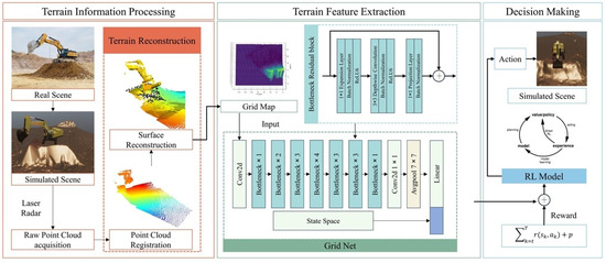
Figure 1.
Overall architecture of E-GTN.
In the terrain information processing stage of our E-GTN framework, we commence with the capture of raw point cloud data using laser radar. These data are then processed using voxel grid downsampling and normal estimation to reduce complexity and enhance feature representation. The resulting downsampled point cloud is essential for creating a detailed and computationally manageable model of the terrain, which is critical for accurate environmental reconstruction and subsequent analysis.
The terrain feature extraction module is the centerpiece of the E-GTN framework, where the downsampled point cloud is meticulously transformed into a structured grid map. This grid map undergoes normalization and is treated as a pseudo-image, allowing us to leverage convolutional neural networks (CNNs) for advanced feature extraction. Our tailored model GridNet adeptly processes the grid data to distill critical terrain features that are instrumental for the reinforcement learning tasks in autonomous excavation.
Finally, the decision-making module utilizes the features extracted by GridNet to inform the reinforcement learning algorithm. While this section is less emphasized, it is still pivotal as it enables the autonomous system to make strategic decisions based on the terrain information provided. The integration of these modules within the E-GTN framework ensures a seamless flow from data acquisition to decision execution, facilitating efficient and intelligent autonomous excavator operations.
3.1. Terrain Information Processing
3.1.1. Raw Point Cloud Acquisition
Given the raw point cloud data P, we apply a voxel grid downsampling method. For each voxel V with edge length l, the subset of points is replaced with their centroid to obtain the downsampled point cloud :
where denotes the number of points in voxel V. The next step involves estimating the normal at each point in . Using a neighborhood defined by a radius search in a KD-tree structure [11], the normal vector at point p is computed as the eigenvector corresponding to the smallest eigenvalue of the covariance matrix constructed from the neighbors of p.
For feature description, we compute Fast Point Feature Histograms (FPFHs) [12] for each point p in based on the normal vectors and the relative positions within a neighborhood :
where is the Simplified Point Feature Histogram for point p, is the inverse Euclidean distance between p and , and k is the number of neighbors.
To align the point clouds into a common coordinate frame, we first apply an initial rough alignment using feature matching. A RANSAC-based approach with FPFH features estimates the transformation by maximizing the consensus set of matched features:
where is the downsampled point cloud from the other laser scanner and is a threshold for matching.
Subsequently, the Iterative Closest Point (ICP) algorithm [13] refines the transformation by minimizing the mean squared error between the corresponding points:
where is the set of corresponding point pairs between the registered point cloud and the target cloud , and is the optimized transformation. Through these steps, we ensure the integrity and computational efficiency of the data, leading to a high-fidelity reconstruction of the excavation site suitable for further simulation and analysis.
3.1.2. Environment Reconstruction
In our study, the region of interest (ROI) is delineated by an axis-aligned bounding box to focus on terrain changes in front of the excavator bucket. The ROI is defined by coordinates and , significantly reducing data processing volume and increasing efficiency.
The Poisson Surface Reconstruction algorithm [14] seeks a smooth surface that approximates the normals of the point cloud. The mathematical formulation involves solving the Poisson equation:
where f is the scalar field whose gradient approximates the point cloud normals , is the Laplacian, and div is the divergence operator. The normals are estimated from the input point cloud, and the divergence of forms the right-hand side of the equation, representing the flux of the normal vectors.
The boundary conditions for the domain are typically set to Neumann conditions:
where is the derivative of f in the direction of the outward normal on the boundary .
After solving the Poisson equation, the surface S is extracted as the isosurface where the scalar field f equals a chosen iso-value , typically zero:
resulting in a triangular mesh that represents the continuous surface of the point cloud data. This reconstruction fills gaps and creates a model with uniform density, facilitating further processing and analysis.
3.2. Terrain Feature Extraction
3.2.1. Point Cloud to Grid Dimensionality Reduction Mapping
In the preprocessing phase, the original point cloud data, which include a set of points each with coordinates, intensity, and environmental label, are denoted as , where and . Here, N is the total number of points in the point cloud, represents the intensity, and is the label of the i-th point.
Filtering based on the label l retains only the points associated with the target environment, resulting in a reduced point cloud , where and . Here, is the count of points in the filtered point cloud.
The grid map parameters are computed as follows:
where W and H are the width and height of the scene, respectively, and and are the grid resolutions in the respective dimensions. An empty grid map is initialized with zero values:
For each point within the specified range, the corresponding grid indices are calculated by:
where and are the minimum coordinates of the grid. The z-coordinate is mapped to the grid if it falls within the specified range :
The grid is then reshaped into a vector for efficient storage and processing:
For visualization and further analysis, the grid map is normalized and converted into a pseudo-image :
This pseudo-image is then scaled to the range [0, 1] to standardize the data for subsequent processing steps:
The normalized grid map is now ready for feature extraction and environmental perception tasks, providing a consistent input for machine learning algorithms.
3.2.2. Terrain Feature Extraction Network
To facilitate the processing of grid data by convolutional neural networks (CNNs), which are typically designed for RGB images, the channel dimension of the grid data must be expanded to simulate a three-channel image. This expansion is denoted by the operation , which replicates the single-channel grid pseudo-image across three channels, yielding a tensor with dimensions , where and represent the height and width of the grid, respectively:
For batch processing, the tensor is further extended to accommodate a batch size of , resulting in a four-dimensional tensor :
The environmental state vector is defined to encapsulate additional necessary inputs from the environment, excluding the target point cloud. It is represented as , where is the dimensionality of the state information.
The feature extraction network, denoted as GridNet, is composed of a CNN model for processing grid data and a fully connected network for processing state data. The CNN model, incorporating depthwise separable convolutions and an inverted residual structure, transforms the input dimensions as follows:
where represents the number of feature channels produced by the CNN. The fully connected network processes the state vector:
where is the size of the feature vector for the state data.
The environmental feature vector is obtained by concatenating the output of the CNN and FCN models:
MobileNetV2 [15] is selected for its efficiency and is specifically adapted for this application. This structure initially expands the channel count of the input feature map through a lightweight expansion layer. It elevates the dimensions before applying depthwise separable convolutions for feature extraction. Finally, a linear projection layer reduces the dimensions back to the original size.
3.3. Decision Making
Within the scope of excavator operations, we confront the dynamic optimization challenge by conceptualizing the joint optimization of excavation strategies as an MDP [16]. To effectively address this MDP, we engineered an adept DRL [17] algorithm. This algorithm is specifically tailored to navigate the intricacies of continuous excavation tasks, thereby refining the decision-making process in a real-time setting.
The MDP framework of our DRL model is succinctly encapsulated by the tuple , where S delineates the state space, A signifies the action space, P represents the set of state transition probabilities, and r constitutes the reward function.
3.3.1. State Space
At any decision epoch t, the state space is formulated to provide a detailed depiction of the excavator’s operational status and its environmental engagement. The state space is concisely defined as:
where encompasses the joint angles of the excavator, entails the angular velocities of the joints, and quantifies the volume of soil excavated at time t.
Given the continuum of the state space, we model the state transition probability as a probability density function f, which quantifies the probability of migrating to the subsequent state consequent to executing an action :
3.3.2. Action Space
The action space , at time t, is comprised of a series of potential excavator movements, each represented by the discrete adjustments in the joint angles:
Each component of specifies an incremental modification to a corresponding joint angle, thereby facilitating precise control over the excavator’s movements and excavation activities.
4. Experiments
4.1. Data Acquisition
Data for our study were sourced from actual excavation sites, as depicted in Figure 2a. The data collection involved an SY870 excavator [18] performing earthmoving tasks, with the operator ensuring consistent excavation criteria and ground leveling post-operation. The SY870 excavator is manufactured by Sany Group, headquartered in Changsha, China. The excavator’s position remained fixed during the tasks, and the terrain was restored after each session to maintain consistent conditions for every new excavation. The SY870 is a hefty machine with a 4.5 cubic meter bucket capacity. In the unloading phase, excavated soil was loaded into mining trucks.
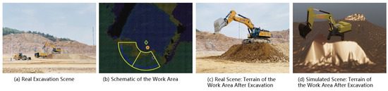
Figure 2.
Excavation operation: Real to simulated.
Throughout the excavation processes, the excavator’s location was kept constant. The operator used a uniform standard to determine the end of the excavation process. The goal was to keep the post-excavation ground as level as possible and to ensure a constant excavation speed. To avoid operational anomalies, the operator restored the terrain after each excavation to ensure the initial conditions for subsequent operations were as consistent as possible. Figure 2b shows the work area of the excavation operation, with Area A being the excavation zone and Area B being the unloading zone. The width of the spoil platform at the excavation site was 13 m, and the work area was 6.5 m by 1.4 m by 4 m.
To simulate actual operations, radar devices were installed on both sides of the excavator’s cabin and boom to collect real-time data about the surrounding environment and terrain. The excavator’s LiDAR is the Ouster OS1. The Ouster OS1 is manufactured by Ouster, Inc., headquartered in San Francisco, CA, USA. This is a high-performance LiDAR with a detection range of up to 100 m and an angular sampling accuracy of vertically and horizontally. The excavator’s four joint angles are fitted with IMU SYD T500 sensors. The manufacturer of the IMU SYD T500 sensors is SYD Dynamics, based in Odense, Southern Denmark. This is an integrated inertial measurement unit that incorporates multiple sensors, capable of outputting measurements from a 3-axis gyroscope and a 3-axis accelerometer with a timestamp resolution of less than 1 μs. During operations, these data were stored at a frequency of 50 Hz in Rosbag packages. The dataset includes the angular velocity of each joint of the excavator, joint force, piston rod speed, volume of soil excavated, ground support force, and LIDAR point clouds. The operator’s excavation trajectory, followed during the operation, was transmitted to a simulation platform (Unity) via the UDP protocol in Matlab 2023a to acquire data on the excavation process in a simulated environment. Figure 2c illustrates the terrain of the work area after the completion of the excavation in the real scenario. Figure 2d displays the terrain of the work area after the excavation in the simulated scenario, which is essentially consistent with the terrain in the real scenario.
4.2. Environment Reconstruction
After capturing the original point cloud data, we processed the terrain information based on the point cloud. The process began with preliminary steps, such as downsampling, normal estimation, and FPFH feature extraction. This was followed by initial registration and then precise alignment using the ICP method for the point clouds collected by the left and right radars of the bucket. Next, we reconstructed the point cloud by first removing outliers and any unreasonable points. We then defined the ROI for the actual excavation process. After selecting the ROI, we used Poisson surface reconstruction techniques to rebuild the point cloud, filling in gaps and preparing for the conversion of the point cloud to a grid and feature extraction.
Our methodology employed the OpenCV library for normal estimation and point cloud registration. This approach facilitated rapid neighborhood searches and maintained a balance between accuracy and computational efficiency.
The preliminary registration aimed to align the left and right radar point clouds roughly, setting the stage for more precise alignment. We utilized OpenCV’s feature-based method to quickly estimate an initial transformation matrix.
For fine-tuning the alignment, we applied the ICP algorithm, optimizing the point clouds’ alignment accuracy. The processed point clouds, an initial transformation from the preliminary step, and a set maximum distance for corresponding points were fed into OpenCV’s ICP implementation. This step refined the point clouds’ alignment by minimizing the direct Euclidean distance between corresponding points.
Figure 3a shows the unregistered point clouds from the left and right radars, where the misalignment is evident. Figure 3b illustrates the point clouds after preliminary registration, showing basic alignment. After ICP registration, as shown in Figure 3c, the left and right point clouds are well aligned, resulting in a fused point cloud.
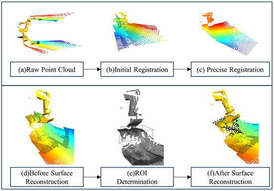
Figure 3.
Terrain reconstruction based on point cloud.
In our research, we focused on the terrain changes in front of the excavator bucket before and after each scoop. In Open3D, we created an axis-aligned bounding box as the ROI to study the terrain changes in detail. As shown in Figure 3e, we defined the ROI boundaries as (3, 2, −4) and (6, 5, 1), with ‘x+’ pointing down and ‘z−’ to the right.
Surface reconstruction organized the points in the point cloud into a smooth surface, effectively representing the continuity and smoothness of the surface. The reconstructed model usually has uniform data density, making the surface features more consistent and continuous. The pre-reconstruction point cloud, as seen in Figure 3d, shows an uneven distribution of points within the ROI and some gaps. After reconstruction, as shown in Figure 3f, the holes and missing parts in the point cloud were filled in, adding points to the area (marked in black), transforming the sparse and incomplete point cloud into a continuous surface model, ready for further modeling operations.
4.3. Terrain Feature Extraction
Firstly, we convert the point cloud into a grid format. The grid map’s width and height are calculated by dividing the real-world scene’s width and height by the resolution. We initialize an empty grid map with the shape (grid_height, grid_width), which corresponds to the size of the grid map. In our study, we focused on a region of interest, selecting a local grid map of (150, 120) with 18,000 grids, representing a 15 m × 12 m real-world scene at a resolution of 0.1 m. We then create an array matching the grid map size, representing the empty grid map as an all-zero array, initializing each grid value to zero. The point cloud ‘lidar’ is then iterated over, mapping the points onto the grid map, uniformly stretching them to fit the grid map. The grid map values are the z-coordinates sampled within each grid’s range, thus reducing the three-dimensional point cloud to a two-dimensional grid map. This pseudo-image, equivalent to a single-channel grayscale image, is then dimensionally expanded by duplication to meet the model’s input requirements, unlike RGB images which have three channels.
Next, we use the MobileNetV2 network as the backbone for GridNet to perform deep learning feature extraction. We select the network’s last layer, extracting image features as a (512, 1) vector, which is then passed through a linear layer to generate a (256, 1) feature vector. This vector encapsulates the basic features of the terrain state, providing a compact yet information-rich representation. These vectors are particularly suitable as input states for the RL algorithm in the next step of the unmanned excavator’s path generation. Compared to other networks mentioned, MobileNetV2 requires fewer computational resources, has a lower parameter count, and operates efficiently, making it suitable for use on mobile devices. In the final grid information extraction, MobileNetV2 processes a total of 300 scoops, including the first and middle scoops. The extracted grid feature information and state feature information are then input into the reinforcement learning model.
This section details training and testing the Decision Transformer (DT) [19], an offline RL algorithm, for generating excavator trajectories. The DT model handles sequence lengths up to 40 and segments up to 200, accommodating the unpredictable data lengths in real-world applications. Its linear embedding layer, operating in a 512-dimensional space, and a decoder with three layers and eight attention heads each, allow for detailed input representation. The model uses a tanh function for action outputs within a continuous range and employs a 0.1 dropout rate for robustness against overfitting. ReLU activations facilitate learning complex patterns. Training datasets with varied segment lengths are batch-sampled and preprocessed. Actions are scaled between −1 and 1, with states and features standardized. The AdamW optimizer, with a learning rate and weight decay of , progressively increases the rate over 100 iterations. A custom loop minimizes the error between predicted and actual actions across 500 iterations of 100 steps each.
The trend in the training loss statistics for the algorithm is indicative of its learning performance. As shown in Figure 4, the mean training loss (a) decreases significantly in the initial steps, suggesting rapid learning and model improvement. The loss continues to gradually decrease, stabilizing towards the end of the training process, which is a sign of the model converging to a solution. The standard deviation of the training loss (b) exhibits a few peaks, which indicates variability in the loss across different training batches. However, similar to the mean, the standard deviation generally decreases over time, implying that the model’s predictions are becoming more consistent as training progresses.
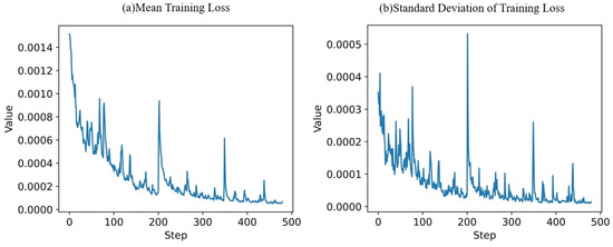
Figure 4.
Model training loss.
5. Results
5.1. Decision-Making Results
The excavator’s decision-making process is a real-time and multi-channel processing dynamic system, as shown in Figure 5. It involves three primary channels: the terrain reconstruction channel (Channel 1), the excavator control channel (Channel 2), and the DRL model operation channel (Channel 3).
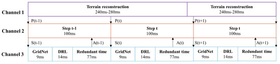
Figure 5.
Real-time decision-making process.
Channel 1: This channel employs two LIDAR scanners to capture point cloud data P(t), which are then used to create a 3D reconstruction of the terrain using the algorithm described in Section 4.2. The processing time for terrain reconstruction ranges from 240 ms to 280 ms.
Channel 2: Operating at a frequency of 10 Hz, this channel executes every 100 ms. At each time step t, it receives the point cloud information P(t) from the terrain reconstruction channel and the current joint information of the excavator, combining them to form the state S(t), which encompasses the immediate conditions of both the environment and the excavator.
Channel 3: The state S(t) is relayed to the DRL model operation channel where it first undergoes processing by the GridNet, taking 9 ms, followed by decision making through the DRL model, which takes 14 ms. Ultimately, the DRL model outputs an action A(t), a vector containing increments for four joint angles, to guide the excavator’s subsequent movement.
The complete operational results of the E-GTN are depicted in Figure 6. Within the simulated environment, the excavator’s bucket has a capacity of 4.5 cubic meters. Under the implementation of our method, coupled with the GridNet’s terrain feature extraction, the system achieved an average excavation volume of 3.7 cubic meters per scoop with a standard deviation of 0.27 cubic meters. In contrast, without the feature extraction, the average excavation volume dropped significantly to 0.45 cubic meters per scoop, with a standard deviation of 0.46 cubic meters. These findings underscore the efficacy of integrating GridNet in enhancing the precision of the excavation process, optimizing the excavator’s operational capacity, and highlighting the importance of terrain feature extraction in the decision-making process.
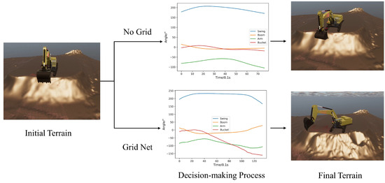
Figure 6.
Excavation result based on EGTN.
5.2. Feature Extraction Results
Upon completing the training, we extracted the terrain features before and after excavation and input them into our GridNet. The visualized results are shown in Figure 7. A comparison between the feature maps before and after training reveals a noticeable difference: post-training, there is an increased level of feature activation, indicating that the network’s ability to extract features has improved.
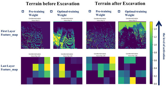
Figure 7.
Comparison of feature map activations.
The images on the left represent the terrain before excavation, while the images on the right depict the terrain after excavation. In both cases, the feature maps are shown for pre-training and optimal-training weights. For the first layer feature maps, the pre-training images are more chaotic and less defined, while the optimal-training images show more distinct patterns and clearer feature representations. This suggests that the network has learned to emphasize relevant features for the task at hand.
Similarly, the last layer feature maps exhibit a stark contrast. The pre-training images are almost uniform with little to no distinctive features, whereas the optimal-training images display well-defined, high-activation regions. This signifies that the network, after training, can better identify and highlight the most critical features of the terrain.
The scale on the right indicates the level of activation, with higher values corresponding to stronger activations. The optimal-training feature maps generally show higher activation levels compared to the pre-training ones, which is a strong indicator of the network’s enhanced feature extraction capability after training.
In our study, we employed principal component analysis (PCA) as a preliminary method to assess the effectiveness of feature extraction by GridNet. Figure 8b presents the PCA results of the feature vectors extracted by GridNet. The first two principal components account for an explained variance ratio of 0.39 and 0.16, respectively, cumulatively explaining over 50% of the variance. The scatter plot associated with these components shows a relative dispersion of data points, lacking a clear clustering trend. This dispersion suggests that the extracted features have a high level of complexity and may capture more nuanced variations within the data.
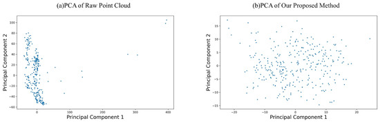
Figure 8.
Comparison of feature map activations.
Conversely, Figure 8a illustrates the PCA results of the raw grid data. Here, the first two principal components have an explained variance ratio of 0.25 and 0.19, which together explain less than 50% of the total variance. The scatter plot reveals a concentrated distribution of data points, indicating a strong clustering tendency. This concentration implies that the raw data may inherently contain less complexity or fewer distinct patterns before the application of feature extraction techniques.
The comparative analysis of the PCA results before and after the application of GridNet allows us to infer that the feature extraction process not only accounts for a greater proportion of the variance but also increases the complexity of the feature representation. This is indicated by the spread of data points in the scatter plot post-extraction, which contrasts with the more clustered distribution seen in the raw data. The ability of GridNet to elucidate a higher amount of variance and to disperse the data points suggests that it is capturing more significant variables within the dataset.
The feature extraction process through GridNet, as evidenced by the PCA, appears to be effective in distilling important variables from the data. This is an encouraging sign that the network can isolate and amplify aspects of the data that are most informative for subsequent analysis. The increased complexity and variance explained by the extracted features are indicative of GridNet’s robustness in representing terrain data in a way that is conducive to advanced terrain analysis and decision-making processes in automated systems.
6. Conclusions
In conclusion, our E-GTN framework has proven to be a robust solution to the challenges posed by unmanned excavator operations. By integrating advanced multisensor fusion, we have significantly enhanced the geometric representation of the terrain, which is foundational for high-fidelity environmental reconstruction. Our GridNet has successfully processed grid data to extract salient terrain features, demonstrating its critical role in the reinforcement learning tasks for autonomous excavation. The decision-making module, informed by these extracted features, has facilitated efficient and intelligent operation, showcasing the potential of our framework to revolutionize the construction machinery industry. The successful application of our E-GTN framework underscores its value as a comprehensive platform for scholars and practitioners in related fields, paving the way for future advancements in autonomous excavation technologies.
Expanding on our work, future iterations of the E-GTN framework could employ adaptive algorithms for better performance across varied soils. Real-time learning capabilities may enable self-optimizing excavators. Additionally, deploying this technology in extreme settings, like underwater or underground, could redefine automated digging. These forward-looking applications not only build on the current strengths of the E-GTN framework but also chart a course for its evolution, solidifying its role as a transformative force in the industry.
Author Contributions
Conceptualization: Q.Z.; methodology: Q.Z., D.W. and X.M.; formal analysis and investigation: Q.Z. and D.W.; writing—original draft preparation: Q.Z.; writing—review and editing: J.Q. and J.H.; funding acquisition: L.G. and J.H.; resources: L.G.; supervision: J.H. All authors have read and agreed to the published version of the manuscript.
Funding
This research is supported by the National Natural Science Foundation of China (52035007, U23B20102), Ministry of Education “Human Factors and Ergonomics” University Industry Collaborative Education Project (No. 202209LH16) and the Xie Youbai Design Scientific Research Foundation (XYB-DS-202401).
Institutional Review Board Statement
Not applicable.
Informed Consent Statement
Not applicable.
Data Availability Statement
Data are available on request to the authors.
Acknowledgments
We would like to extend our sincere thanks to Sany Company for their support and contribution to this research.
Conflicts of Interest
Author Le Gao was employed by the company Sany Heavy Machinery Co., Ltd. The remaining authors declare that the research was conducted in the absence of any commercial or financial relationships that could be construed as a potential conflict of interest.
References
- Hemami, A.; Hassani, F. An overview of autonomous loading of bulk material. In Proceedings of the 26th International Symposium on Automation and Robotics in Construction, Austin, TX, USA, 24–27 June 2009; International Association for Automation and Robotics in Construction (IAARC): Austin, TX, USA, 2009; pp. 405–411. [Google Scholar]
- Dadhich, S.; Bodin, U.; Andersson, U. Key challenges in automation of earth-moving machines. Autom. Constr. 2016, 68, 212–222. [Google Scholar] [CrossRef]
- Zhang, L.; Zhao, J.; Long, P.; Wang, L.; Qian, L.; Lu, F.; Song, X.; Manocha, D. An autonomous excavator system for material loading tasks. Sci. Robot. 2021, 6, eabc3164. [Google Scholar] [CrossRef] [PubMed]
- IndustryResearch. Global Excavator Market Report. 2020. Available online: https://www.industryresearch.co/global-excavator-market-18836753 (accessed on 30 March 2024).
- Afshar, R.R.; Zhang, Y.; Vanschoren, J.; Kaymak, U. Automated reinforcement learning: An overview. arXiv 2022, arXiv:2201.05000. [Google Scholar]
- Stentz, A.; Bares, J.; Singh, S.; Rowe, P. A robotic excavator for autonomous truck loading. Auton. Robot. 1999, 7, 175–186. [Google Scholar] [CrossRef]
- Yamamoto, H.; Moteki, M.; Ootuki, T.; Yanagisawa, Y.; Nozue, A.; Yamaguchi, T. Development of the autonomous hydraulic excavator prototype using 3-D information for motion planning and control. Trans. Soc. Instrum. Control. Eng. 2012, 48, 488–497. [Google Scholar] [CrossRef]
- Chae, M.J.; Lee, G.W.; Kim, J.Y.; Park, J.W.; Cho, M.Y. A 3D surface modeling system for intelligent excavation system. Autom. Constr. 2011, 20, 808–817. [Google Scholar] [CrossRef]
- Shariati, H.; Yeraliyev, A.; Terai, B.; Tafazoli, S.; Ramezani, M. Towards autonomous mining via intelligent excavators. In Proceedings of the IEEE/CVF Conference on Computer Vision and Pattern Recognition Workshops, Long Beach, CA, USA, 16–17 June 2019; pp. 26–32. [Google Scholar]
- Forkel, B.; Kallwies, J.; Wuensche, H.J. Probabilistic terrain estimation for autonomous off-road driving. In Proceedings of the 2021 IEEE International Conference on Robotics and Automation (ICRA), Xi’an, China, 30 May–5 June 2021; IEEE: Piscataway, NJ, USA, 2021; pp. 13864–13870. [Google Scholar]
- Foley, T.; Sugerman, J. KD-tree acceleration structures for a GPU raytracer. In Proceedings of the ACM SIGGRAPH/EUROGRAPHICS Conference on Graphics Hardware, Los Angeles, CA, USA, 30–31 July 2005; pp. 15–22. [Google Scholar]
- Rusu, R.B.; Blodow, N.; Beetz, M. Fast point feature histograms (FPFH) for 3D registration. In Proceedings of the 2009 IEEE International Conference on Robotics and Automation, Kobe, Japan, 12–17 May 2009; IEEE: Piscataway, NJ, USA, 2009; pp. 3212–3217. [Google Scholar]
- Chetverikov, D.; Svirko, D.; Stepanov, D.; Krsek, P. The trimmed iterative closest point algorithm. In Proceedings of the 2002 International Conference on Pattern Recognition, Quebec, QC, Canada, 11–15 August 2002; IEEE: Piscataway, NJ, USA, 2002; Volume 3, pp. 545–548. [Google Scholar]
- Kazhdan, M.; Bolitho, M.; Hoppe, H. Poisson surface reconstruction. In Proceedings of the Fourth Eurographics Symposium on Geometry Processing, Cagliari, Italy, 26–28 June 2006; Volume 7. [Google Scholar]
- Sandler, M.; Howard, A.; Zhu, M.; Zhmoginov, A.; Chen, L.C. Mobilenetv2: Inverted residuals and linear bottlenecks. In Proceedings of the IEEE Conference on Computer Vision and Pattern Recognition, Salt Lake City, UT, USA, 18–22 June 2018; pp. 4510–4520. [Google Scholar]
- Parkes, D.C.; Singh, S. An MDP-based approach to online mechanism design. In Advances in Neural Information Processing Systems 16: Proceedings of the 2003 Conference; MIT Press: Cambridge, MA, USA, 2003. [Google Scholar]
- François-Lavet, V.; Henderson, P.; Islam, R.; Bellemare, M.G.; Pineau, J. An introduction to deep reinforcement learning. Found. Trends® Mach. Learn. 2018, 11, 219–354. [Google Scholar] [CrossRef]
- SY750H | Large Excavator. 2024. Available online: https://www.sanyglobal.com/product/excavator/large_excavator/115/847/ (accessed on 30 March 2024).
- Chen, L.; Lu, K.; Rajeswaran, A.; Lee, K.; Grover, A.; Laskin, M.; Abbeel, P.; Srinivas, A.; Mordatch, I. Decision transformer: Reinforcement learning via sequence modeling. Adv. Neural Inf. Process. Syst. 2021, 34, 15084–15097. [Google Scholar]


Disclaimer/Publisher’s Note: The statements, opinions and data contained in all publications are solely those of the individual author(s) and contributor(s) and not of MDPI and/or the editor(s). MDPI and/or the editor(s) disclaim responsibility for any injury to people or property resulting from any ideas, methods, instructions or products referred to in the content. |
© 2024 by the authors. Licensee MDPI, Basel, Switzerland. This article is an open access article distributed under the terms and conditions of the Creative Commons Attribution (CC BY) license (https://creativecommons.org/licenses/by/4.0/).