Analysis of Surface Temperature Modified by Atypical Mobility in Mexican Coastal Cities with Warm Climates

Abstract

This study takes a unique approach, using satellite remote sensing to analyze the land surface temperature (LST) in seven coastal cities located at latitudes between 18° and 22° and longitudes between 106° and 91°. The methodology consists of obtaining the LST on two selected days, one in July 2019 and one in July 2020, to determine how the temperature was modified by the atypical mobility caused by Coronavirus Disease 2019 (COVID-19) and social distancing. Using these data, we determine the representative surface temperature that tended to rise (RHST) and the representative surface temperature that tended to decrease (RLST), depending on the affected area. This approach allows us to comprehensively compare how mobility modified the four variables studied: territorial extension, population, types of soil (paving), and vegetation. We concluded that, among the factors analyzed, the types of paving and vegetation were those that generated a more significant decrease in temperature; the variables of territorial extension and the number of inhabitants had a smaller impact. This study paves the way for a discussion of the significant influence of mobility on the behavior of the LST.

1. Introduction

Urban areas have experienced an increase in temperature in their centers compared to their surroundings, a phenomenon known as the urban heat island (UHI) effect. This phenomenon is associated with heightened energy consumption, greenhouse gas emissions, pollution, and increased mortality rates due to prolonged exposure to high temperatures [1]. Urban climatology focuses on studying and understanding the local changes in urban temperatures that result from settlements and urban activities. This discipline enables the creation of thermal maps, which can be used to analyze and monitor urban climatic conditions; this is essential for the adequate planning, rehabilitation, restructuring, or reconstruction of cities, ultimately improving the comfort of their inhabitants [2].

Although our research focuses on analyzing local and spatial variations in land surface temperature (LST) during the day in the city, our intention is to highlight its importance in the context of the Urban Heat Island (UHI) and Surface Urban Heat Island (SUHI) phenomena. By way of definition, and without delving too deeply into the topic, we can say that SUHI represents the difference in LST between urban and suburban areas, and is comparable to the temperature curves of the atmospheric UHI [3]; however, a distinction is made in that the maximum cycle of the UHI occurs during the night, while the SUHI peaks in the middle of the day, since surface temperature is influenced by the effect of solar radiation and the albedo of materials, whereas at night, the release of heat in the nocturnal boundary layer and the reduction of net longwave loss/effective radiation are important processes for the UHI effect [4,5]; it is for this reason that the research is conducted during the day.

A significant advantage of LST is that it can be obtained simultaneously in space and time using satellite information, eliminating the need for data analysis from meteorological stations or conducting transects. The validation of the relationship between UHI and SUHI has been demonstrated in a number of studies [5,6,7,8,9].

Several factors influence the characterization and distribution of atmospheric and surface temperatures in urban areas; these include the physical and thermal properties of surfaces, such as reflectance, albedo, emissivity, and emittance. Green areas also play a critical role by affecting soil evapotranspiration. Furthermore, urban morphology, building density, proportions, land use, and texture significantly impact thermal conditions. Anthropogenic heat generated by industries, buildings, and vehicles contributes to the formation of UHIs. Research on UHIs and SUHIs encompasses studies at various scales, from regions to cities and neighborhoods, aiming to enhance scholarly understanding of the phenomenon and develop resilience strategies. These multidisciplinary studies combine analyses of physical, morphological, and anthropogenic factors to comprehensively address the issue of urban heat islands and propose context-specific solutions.

In the study of SUHIs, meteorological parameters such as the temperature, radiation, relative humidity, and wind speed and direction must be considered. This research focuses on four factors: mobility, population, land area, and the properties of paved surfaces, including the normalized difference vegetation index (NDVI), which have been linked to alterations in SUHI temperatures.

Mobility, or vehicular traffic, is a component of anthropogenic heat, referring to heat generated as a result of human activities. Transportation is generally seen as a solution for mobility in large cities, providing significant societal benefits; however, it has also created negative effects on the environment and urban climatology. Emissions from vehicles and the heat generated by them contribute to heat transfer and radiation between the air and the ground surface [10,11]. Studies have demonstrated a strong correlation between mobility and the SUHI [12,13,14]. For example, research indicates that one of the thermal effects of vehicles is the substitution of atmospheric downwelling infrared radiation (IR) with IR emissions from the underside of the vehicle. Of particular significance are the IR emissions from the heated engine, transmission, and exhaust system directed towards the road surface [15,16,17].

Regarding land area, Zhou et al. [18], analyzed 5000 cities and determined that city size has the strongest influence on the intensity of the SUHI; larger, more compact, and less sprawled cities tend to exhibit stronger SUHI effects. In Europe, the intensity of UHIs in urban agglomerations shows a size dependency, typically reaching a maximum of approximately 3 °C in summer and 0.5 °C in winter [19].

Population density, built density, and vegetation can also directly or indirectly contribute to the formation of SUHIs [20]. A study analyzing 65 cities in North America found that the average annual daytime and nighttime UHI are positively correlated with precipitation and the logarithm of the population, respectively [21]. Research conducted in five cities in Bangladesh, utilizing the LST, determined that the SUHI effect is higher during the day than at night, with a long-term increasing trend [22].

The construction materials used in facades, roofs, and pavements play a vital role in the thermal balance of cities. Pavements predominantly absorb shortwave solar radiation during the day and, depending on their temperature, re-emit longwave radiation into the atmosphere [4]. This process causes the increase in air temperature near the surface during the day to be mainly attributable to turbulent sensible heat flux, specifically through the divergence of said flux. Attention has been paid to albedo in urban construction, as areas with a higher reflectance index, such as reflective permeable surfaces and reflective pavements, present potential strategies for UHI mitigation [23]. A study in Xi’an, the largest city in northwestern China, found that the density of impervious surfaces had a more significant impact on the LST than green space, with a Pearson correlation coefficient ranging from 0.59 to 0.97 [8]. Similarly, in Turin, Italy’s largest metropolitan area, it was calculated that, for every 10% increase in highly impervious surfaces with low tree cover in the metropolitan core, the SUHI increased by 4.0 °C [24].

The loss of soil moisture through direct evaporation and transpiration from vegetation is crucial to the modification of surface temperatures [25]. Changes in vegetation density, height, and surface coverage directly affect the soil surface temperature [26]. The presence of vegetation in urban areas reduces temperatures through evapotranspiration and shading, while paved areas contribute to increased temperatures through radiation heat transfer to the urban atmosphere [27] Using thermal remote sensing, the Normalized Difference Vegetation Index (NDVI) can be calculated from spectrometric data collected in two specific bands: red and near-infrared, which assesses vegetation quality values ranging from −1 to 1. This index has been applied in urban planning to estimate the active photosynthetic biomass density and its impact on normalized urban temperatures [28].

This study utilizes satellite remote sensing methodology to analyze land surface temperature (LST) in seven coastal cities over two days—one in July 2019 and the other in July 2020—focusing on local and spatial temperature variations during the daytime. These cities are located between 18° and 22° latitude and 106° and 91° longitude. Variables such as the land area, population, types of pavements, vegetation, and anthropogenic activities, including mobility, are examined in terms of their impact on the LST.

This research highlights how human behavior influences urban climate, which is crucial for urban planning and environmental management. It aims to verify the significance of these variables for future discussions on heat mitigation strategies through urban policies, including the design of green spaces and the selection of more sustainable building materials. By focusing on coastal cities, the proposal also establishes a framework for comparative studies in other regions, allowing for the evaluation of how local characteristics affect land surface temperature (LST) outcomes.

2. Study Area

We analyzed seven coastal cities with urban areas adjacent to the Pacific Ocean and the Gulf of Mexico. The first group, located on the western side bordering the Pacific Ocean, includes the cities of Puerto Vallarta, Jalisco (Vall), Manzanillo, Colima (Mzn), and Lázaro Cárdenas, Michoacán (LC). The second group, situated on the eastern side bordering the Gulf of Mexico, comprises Tampico, Tamaulipas (Tmp), Veracruz, Veracruz (Vrz), Coatzacoalcos, Veracruz (Ctz), and Ciudad del Carmen, Campeche (CC) (Figure 1).

The selection considers these cities as essential ports with very active tourist activity; these cities therefore have similar characteristics in terms of land use and activities in the urban population.

Table 1. Characteristics of the cities selected for measurement ¹.

City	Latitude	Longitude	Altitude (m)	Climatic Classification	Precipitation (mm)
1. Puerto Vallarta, Jalisco (Vall)	20.6136	−105.227	111	Aw	1385
2. Manzanillo, Colima (Mzn)	19.0522	−104.316	17	Aw	900
3. Lázaro Cárdenas, Michoacán (LC)	17.9561	−102.192	15	Aw	1277
4. Tampico, Tamaulipas (Tmp)	22.2553	−97.8686	39	Aw	916
5. Veracruz, Veracruz (Vrz)	19.1727	−96.1333	11	Aw	1500
6. Coatzacoalcos, Veracruz (Ctz)	18.1378	−94.4353	33	Am	3000
7. Ciudad Carmen, Campeche (CC)	18.2672	−91.8001	3	Aw	1155

¹ Free-access information from the Mexican government [30,31,32,33,34,35,36] was used to determine the climatic classification of the analyzed cities based on Köppen–Geiger world maps, where Aw is Tropical–Rainforest and Am is Tropical–Monsoon [37].

shows their geographical characteristics and general data.

The ambient temperature behavior in the selected cities, based on information obtained from official meteorological stations [36], is presented in

Table 2. Monthly average temperatures for June and July of 2019 and 2020, along with the selected days for comparison; they exhibit stable conditions and provide adequate information from the satellite [36].

City	June 2019 (°C)	July 2019 (°C)	June 2020 (°C)	July 2020 (°C)	Days Selected for Comparative Analysis
1. Puerto Vallarta, Jalisco (Vall)	29.30	29.17	29.05	28.70	4 July 2019	22 July 2020
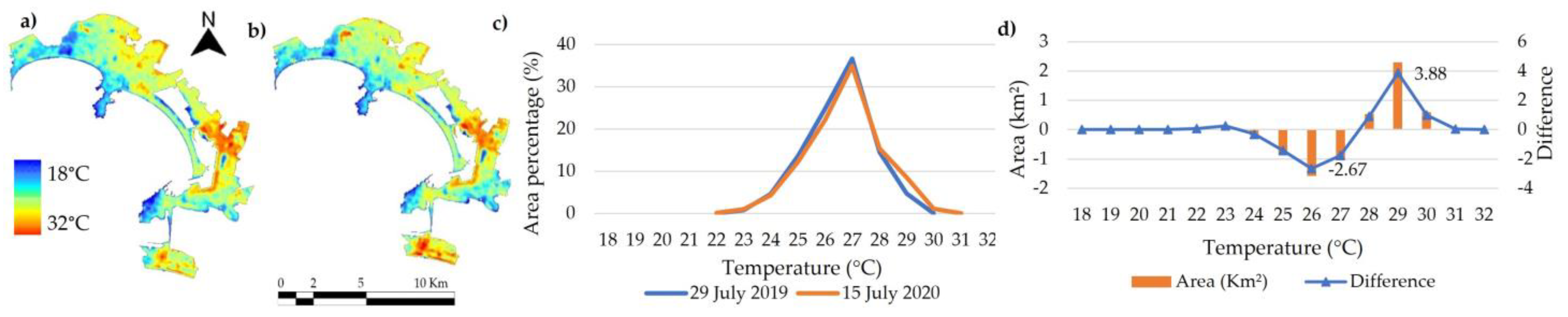
2. Manzanillo, Colima (Mzn)	28.74	29.50	29.41	28.91	29 July 2019	15 July 2020
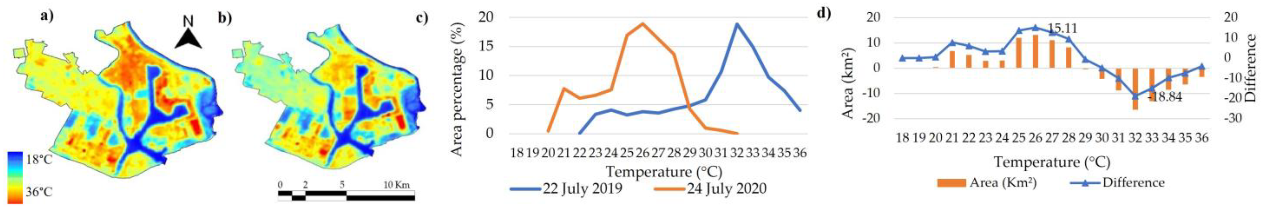
3. Lázaro Cárdenas, Michoacán (LC)	29.67	29.51	29.20	28.55	22 July 2019	24 July 2020
4. Tampico, Tamaulipas (Tmp)	29.26	29.08	29.70	28.48	8 July 2019	10 July 2020
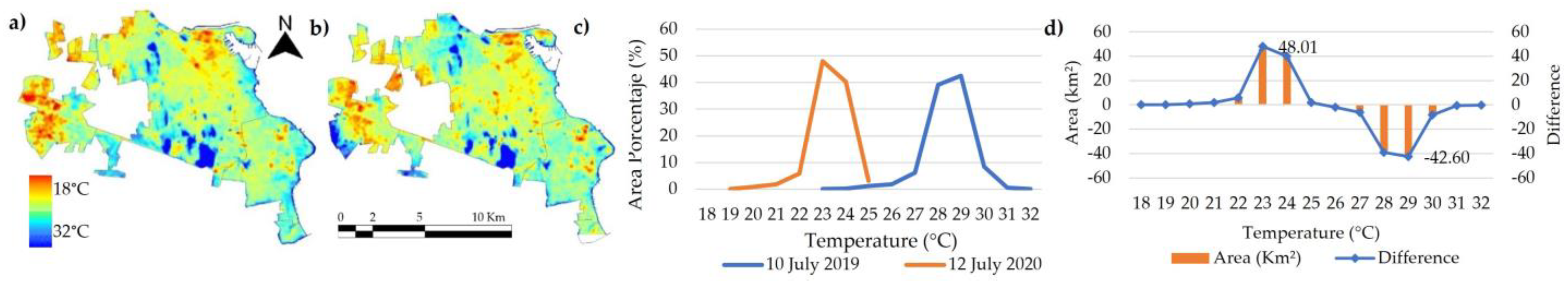
5. Veracruz, Veracruz (Vrz)	28.49	27.98	28.12	27.98	10 July 2019	12 July 2020
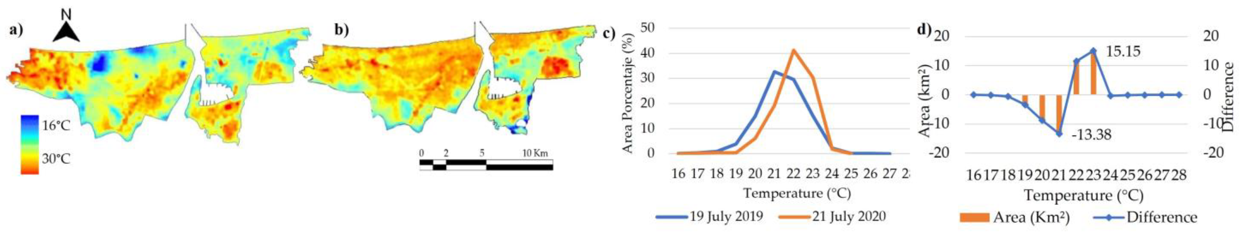
6. Coatzacoalcos, Veracruz (Ctz)	28.20	28.02	27.92	27.33	19 July 2019	21 July 2020
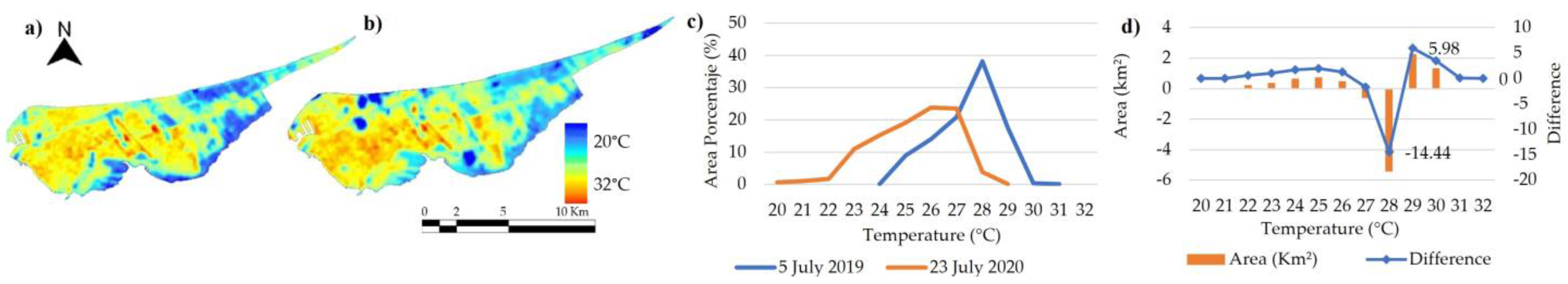
7. Ciudad Carmen, Campeche (CC)	28.78	28.57	28.58	28.21	5 July 2019	23 July 2020

. The table shows the average monthly temperature data for June and July of 2019 and 2020, limited to the study period; it enables us to determine that their behavior is similar.

However, since the LandSat8 satellite crosses approximately twice per month in the same quadrant, those images must show stable weather conditions, and clear skies should be selected. The days selected for analysis, which fall in the summer period in 2019 and 2020, are shown in Table 2.

Our research comprehensively explores the profound impact of mobility on urban thermal patterns, using 2019 and 2020 as comparative years. The year 2020, marked by a global decline in mobility due to the Coronavirus Disease 2019 (COVID-19) pandemic, saw significant changes in travel and crowd avoidance behaviors [38]. This shift in mobility behaviors has profound implications for our understanding of urban thermal dynamics.

The mobility index is a measure of the movement of people in a specific area. For the analysis of Mexico’s ‘Sana Distancia Program’ during the COVID-19 pandemic, this index was determined using anonymized geolocation data from telecommunications and mobile applications. These data were compared with mobility patterns starting from 15 February 2020, to identify changes in behavior. The mobility categories included trips to workplaces, residential areas, parks, stores, and entertainment centers. This index allowed authorities to assess the effectiveness of lockdowns and other social distancing measures and to adjust policies according to the need to control the spread of the virus.

Figure 2 shows the percentage change in mobility behaviors by state over a 24-week analysis period. The report concludes that the states of Jalisco, Colima, Michoacán, Tamaulipas, Veracruz, and Campeche decreased their mobility from 15 February 2020, to 29 July 2020, by 43%, 47%, 45%, 51%, 47%, and 58%, respectively [39].

As shown in Figure 3, we meticulously analyzed data from the National Housing Inventory of the National Institute of Statistics and Geography (INEGI) to identify the various types of pavements that form Mexican cities and their distribution within the urban area. The pavements were methodically classified into (a) concrete or asphalt pavements (referred to as highly impermeable), (b) a combination of concrete, asphalt, and paved earth (moderately impervious), and (c) paved earthy or arid soils (slightly impervious) [30].

Using this comprehensive information and with the aid of bidimensional drawing Autocad software (Version T.53.0.0 Autocad 2023), we determined the coverage percentage of each pavement. The results, which demonstrate our thorough classification process, are detailed in

Table 3. Percentage of pavement types in the cities analyzed ³.

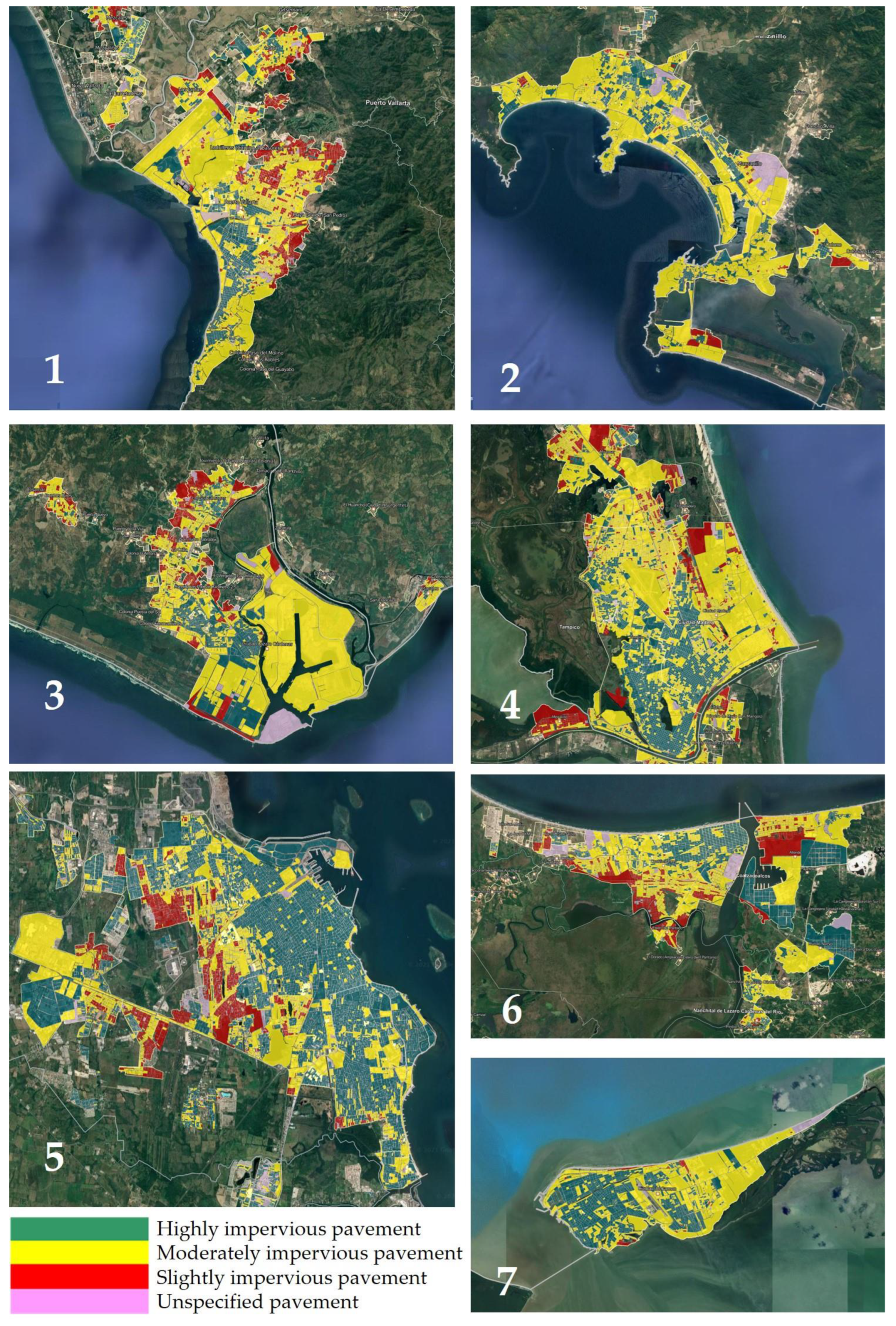
City	Highly Impermeable (%)	Moderately Impervious (%)	Slightly Impervious (%)	No Data (%)
1. Puerto Vallarta, Jalisco (Vall)	17	67	13	2
2. Manzanillo, Colima (Mzn)	18	70	3	9
3. Lázaro Cárdenas, Michoacán (LC)	17	72	6	5
4. Tampico, Tamaulipas (Tmp)	11	47	28	14
5. Veracruz, Veracruz (Vrz)	46	34	13	7
6. Coatzacoalcos, Veracruz (Ctz)	29	49	18	4
7. Ciudad Carmen, Campeche (CC)	31	37	17	15

³ Modified and analyzed results from the data of the National Institute of Statistics and Geography [30].

.

3. Methodology

The launch of satellites into orbit in recent decades has enabled the observation and monitoring of the Earth’s surface for various scientific objectives, including meteorological conditions. The resolution of satellites is contingent upon their altitude and type, whether that is polar or geostationary. Unlike geostationary satellites, polar satellites have lower temporal resolution; they capture images of the same area at specific intervals but offer higher spatial resolution due to their lower orbital altitude [40]. The data for this analysis are sourced from Landsat 8, a polar satellite that orbits at an altitude of 705 km.

The utilization of publicly accessible data from Landsat 8 provides a fine spatial resolution of 100 × 100 m². Additionally, a well-established calculation methodology is employed to derive the land surface temperature (LST) [41]. Continuous improvements in the satellite’s algorithms for processing thermal bands, as provided by its thermal infrared sensor (TIRS), further enhance data reliability, supported by rigorous validation from multiple researchers [8,42,43,44].

Satellites typically pass over the same area twice per month; therefore, it is essential to analyze the images generated to ensure stable climatic conditions and clear skies, in order to avoid interference with the results. This information facilitates the estimation of surface temperatures for various urban features, including roofs, pavements, and types of land use, covering micro-scales such as streets and canyons, as well as medium and macro scales or regions [45,46,47,48]. The wavelengths measured using remote sensors fall within the thermal band, encompassing ultraviolet radiation, visible light, and infrared rays, with a range from 0.1 mm to 100 mm. At this juncture, the Stefan–Boltzmann Law is applied, allowing for the calculation of radiation from a hot body to a cooler environment (Equations (1) and (2)) [49]:

$$E=\sigma T^4$$

(1)

$$E=\epsilon \sigma \left(T^4-T_C^4\right)$$

(2)

where:

• σ = The Stefan–Boltzmann constant 5.67 × 10⁻⁸ W/(m² K⁴);
• ε = The emissivity of the surface;
• T = The absolute temperature of the object (°K);
• Tc = The absolute temperature of the environment (°K).

These remote surveys, which identify temperature peaks, assume that land surface temperature patterns correlate with air temperature patterns. To acquire satellite data, users must access the official website of the United States Geological Survey (https://earthexplorer.usgs.gov/ (accessed on 22 February 2024)). The process can be divided into four steps: (a) search for the selected analysis site by entering latitude and longitude coordinates; (b) specify the period for analysis; (c) utilize LANDSAT COLLECTION 1 LEVEL-1, with additional criteria of Operational Land Imager (OLI)/TIRS C1 LEVEL 1; and (d) download the group of files to obtain a compressed folder containing all the necessary files for processing in ArcGIS.

The data acquired from the Landsat 8 satellite include digital numbers from the Operational Land Imager (OLI) and the Mono-Window Algorithm (MWA), which translates surface temperature using bands 10 and 11. This process incorporates parameters established in the downloaded data, including the average atmospheric temperature, brightness temperature, atmospheric transmittance, and emissivity of the land surface [50,51,52]. These thermal infrared images are subsequently processed using geographic information system (GIS) software (ArcGis Desktop 10.8 Version 10.7.0.10450) to derive values for radiance, the NDVI (normalized difference vegetation index), reflectance, and ultimately, the LST.

3.1. Image Processing

Initially, all the images are loaded into ArcGIS^® software (Version 10.8, 2019). This system facilitates the collection, organization, management, analysis, sharing, and distribution of geographic information, creating a new template for displaying satellite images of the analyzed cities. The first step involves removing the “background” of bands 4, 5, and 10 using the Raster Calculator tool in the ArcToolbox/Spatial Analyst Tools/Map Algebra section (Equation (3)). This procedure is repeated for all three bands.

$$BAND{S}_{\mathrm{4,5}}and10=Setnull\left(“SelectBand”=0,“SelectBand”\right)$$

(3)

Upon completion of this step, the study area is clipped to an appropriate scale using the CLIP tool in the Windows/Image Analysis section. All bands must be selected, including those processed prior to clipping. After clipping the bands for the study area, a new red, blue, green (RGB) layer is created using the Composite Bands tool, located in Windows/Image Analysis. Only bands 2, 3, and 4, resulting from the clipping, are selected. Once the command is applied, a new RGB layer is generated, which must be configured by rearranging the bands in the order b4/b3/b2, within their properties.

Following these processes, calculations are performed to obtain the radiance of the thermal images. For this calculation, bands B10 and B11 are processed using the Raster Calculator tool. The equation utilized (Equation (4)) requires the values of Bands 10 and 11, which can be found in the attribute table of the root folder, located at the beginning of the table of contents. The values are listed under the names RADIANCE MULT_BAND_10 and RADIANCE MULT_BAND_11. The constant value of 0.0003342, used in the equation, is derived from the data tables labelled RADIANCE MULT_BAND, which is the standard value for the Landsat 8 satellite.

$$RADIANC{E}_{10}or11=0.0003342\ast ”Band10or11”+0.10$$

(4)

The next value required is the soil brightness temperature, derived from the previously generated bands labeled Radiance_10 or 11. Using the Raster Calculator (RC) tool again, the bands labelled Brightness_10 or 11 are computed (Equations (5) and (6)). The values of 1321.0789 and 1201.1442 are obtained from the attribute table of the root folder, specifically under the following names: (a) K2_CONSTANT_BAND_10 = 1321.0789 and (b) K1_CONSTANT_BAND_10 = 774.8853. Finally, the value of 272.15 is used to convert the final results from degrees Fahrenheit to degrees Celsius. Once both bands are generated, they are averaged using the Cell Statistics tool located in the Windows/Search/Cell Statistics section.

$$BT\_10=1321.0789/Ln(774.8853/”RADIANCE\_10”+1)-273.15$$

(5)

$$BT\_11=1201.1442/Ln(480.8883/”RADIANCE\_11”+1)-273.15$$

(6)

A significant metric in understanding the thermal behavior of urban areas is the normalized difference vegetation index (NDVI), which ranges between 1 and −1. When the spectral response of the Earth’s surface is similar across both bands, NDVI values approach zero, indicating neutral values or no significant changes. Healthy vegetation, characterized by photosynthetic activity, reflects more in the near-infrared spectrum than in the visible spectrum, resulting in positive NDVI values for green vegetation. NDVI values typically range between 0.1 and −0.1, representing areas with little or no vegetation [53,54]. To determine the vegetation level in the study area, bands 5 and 4 are processed using the RC tool (Equation (7)). When processed correctly, selecting a color scale within the green hues is advisable.

$$NDVI=(Float\left(\mathrm{Band}5-Band4\right)/Float\left(Band5+Band4\right)$$

(7)

From the NDVI, the vegetation percentage (VP) is derived. These data are a continuous variable, necessitating the use of previously obtained NDVI values based on their maximum and minimum values (Equation (8)):

$$VP={\left(\right(“NDVI”+NDVIMin)/(NDVIMax–NDVIMin\left)\right)}^2$$

(8)

It is from these final data that we obtain the land surface emissivity (LSE) (Equation (9)):

$$LSE=0.004\ast “VP”+{\epsilon }_G$$

(9)

where the value of 0.004 serves as a factor to adjust emissivity when vegetation is present, provided that the condition VP ≤ 0.5 is met, and εG represents soil emissivity (0.96–0.98).

The land surface temperature (LST) requires the B10 and B11 bands corresponding to the soil brightness temperature; these must be processed using the appropriate equation (Equation (10)). In this final step, averaging is performed using the Cell Statistics tool.

$$LST=B{T}_{10or11}/1+B{T}_{10or11}/\mathrm{14,380}\ast “LSE”$$

(10)

Another essential step for visualizing the created layers involves modifying their properties, such as the color scale, to enhance the visual interpretation of the existing temperatures in the area. For this investigation, a color scale ranging from red to blue was employed, where red indicates the hottest areas in the city, while blue represents the cooler areas or clouds.

3.2. Data Processing

Like the processing conducted using ArcGIS^® software (ArcGis Desktop 10.8 Version 10.7.0.10450), a statistical methodology was applied to generate values for comparison and to draw conclusions. The LST values are presented in the attribute table of that layer, indicating the existing ranges and pixel counts for LST temperatures on the analyzed days in July 2019 and 2020. The database enables the calculation of the area (km²) corresponding to each value range and the determination of the occupancy percentage within each city’s total area. It is notable that this observational approach does not focus on the location of the city’s isotherms but rather on the overall ranges of the LST. Figure 4, Figure 5, Figure 6, Figure 7, Figure 8 and Figure 9, and with letters a and b display the images obtained from ArcGIS^®.

The attribute table of the NDVI layer, similarly to the LST, presents its ranges and frequency counts within the analyzed area and days. In total, the database for the cities amounted to 52,000 values, leading to the establishment of 20 statistical intervals with a range width of 0.035 (±0.0005), considering that the vegetation index ranges between 1 and −1. The ranges were determined by subtracting the lowest data point from the highest data point and dividing by the proposed number of intervals. Using Excel, the frequency of each interval for each year was calculated. This approach allowed for a more homogeneous analysis of values across cities without compromising their attributes and characteristics. Finally, the occupancy percentage of these values was processed to assess whether the decrease in mobility affected the indicator.

4. Results

The results of the LST in the seven cities are illustrated in Figure 4, Figure 5, Figure 6, Figure 7, Figure 8, Figure 9 and Figure 10. Letters (a) and (b) in Figure 4, Figure 5, Figure 6, Figure 7, Figure 8, Figure 9 and Figure 10 depict the thermal images obtained from satellite data for the two selected days (Table 2), with a resolution of 100 × 100 m per pixel; the images have been edited and cropped to highlight specific areas of the cities.

Figure (c) corresponds to the behavior of the LST, graphically comparing how surface temperatures increase or decrease. Graphs (d) present three variables: the X-axis represents the temperatures recorded in urban areas, the left Y-axis indicates the area in square kilometers where temperature changes occurred between the two days, and the right Y-axis shows the percentage change. This analysis allows for the determination of LST variations.

This research aimed to ensure that meteorological conditions were consistent across all cities, providing us with the opportunity to analyze variables such as land area, population, pavement types, and NDVI in relation to changes in the land surface temperature (LST) associated with a decrease in mobility (greater than 40%) due to the COVID-19 quarantine.

The temperature ranges in the seven cities varied between 18 °C and 32 °C. Notably, two cities exhibited an upward trend (Puerto Vallarta and Tamaulipas), two cities remained relatively stable (Manzanillo and Coatzacoalcos), and three cities demonstrated a downward trend (Lázaro Cárdenas, Veracruz, and Ciudad del Carmen) in terms of surface temperatures (Figure 4, Figure 5, Figure 6, Figure 7, Figure 8, Figure 9 and Figure 10).

The incidence graphs (d) provide two key values: the high and low temperatures that underwent the most significant changes in area within the study cities. These values are designated as the representative high surface temperature (RHST) and the representative low surface temperature (RLST). For example, in Puerto Vallarta, the RLST (23 °C) decreased by 30.79% in area, while the RHST (28 °C) increased by 40.60%; in Tampico, the RLST decreased by 34.12% and the RHST increased by 32.40%; and, in Coatzacoalcos, the RLST decreased by 13.38% and the RHST increased by 15.15%.

Figure 11 illustrates the behavior of the normalized difference vegetation index (NDVI) between two days in 2019 and 2020. The maximum NDVI value observed among the cities was 0.6992, while the minimum was −0.19603; the former corresponds to Coatzacoalcos and the latter to Ciudad del Carmen, both of which are located near the Gulf of Mexico.

Based on the RHST and RLST values (

Table 4. Values utilized in the relationship and linear regression graphs [30,31,32,33,34,35,36].

City	RLST (°C)	ARLST (%)	RHST (°C)	ARHST (%)	Surface (km2)	Population (Inhabitants)	Permeable Pavements (%)	NDVI High
Puerto Vallarta, Jalisco (Vall)	23	−30.79	28	40.60	40.62	291,200	67	0.6295
Manzanillo, Colima (Mzn)	26	−2.67	29	3.88	59.07	184,541	70	0.5819
Lázaro Cárdenas, Michoacán (LC)	26	15.11	32	−18.84	87.29	183,185	72	0.5457
Tampico, Tamaulipas (Tmp)	21	−34.12	28	32.40	92.73	314,418	47	0.5716
Veracruz, Veracruz (Vrz)	23	48.01	29	−42.30	96.09	609,964	34	0.5311
Coatzacoalcos, Veracruz (Ctz)	21	−13.38	23	15.15	50.91	319,187	49	0.6992
Ciudad Carmen, Campeche (CC)	28	−14.44	29	5.98	37.74	248,303	37	0.6091

) obtained from the graph, the coefficient of determination or linear regression is calculated using the variables of land area, population, surface coverage, and vegetation index.

Figure 12, Figure 13, Figure 14, Figure 15, Figure 16, Figure 17 and Figure 18 illustrate the relationships between the representative low surface temperature (RLST) and the representative high surface temperature (RHST) in relation to each variable. The values of the variables are organized from lowest to highest according to their respective ranges, and the corresponding RLST and RHST values are plotted accordingly.

Table 5. R² values and correlation coefficients.

City	Representative Low Surface Temperature (RLST) Representative High Surface Temperature (RHST)
	RHST (R2)	RLST (R2)
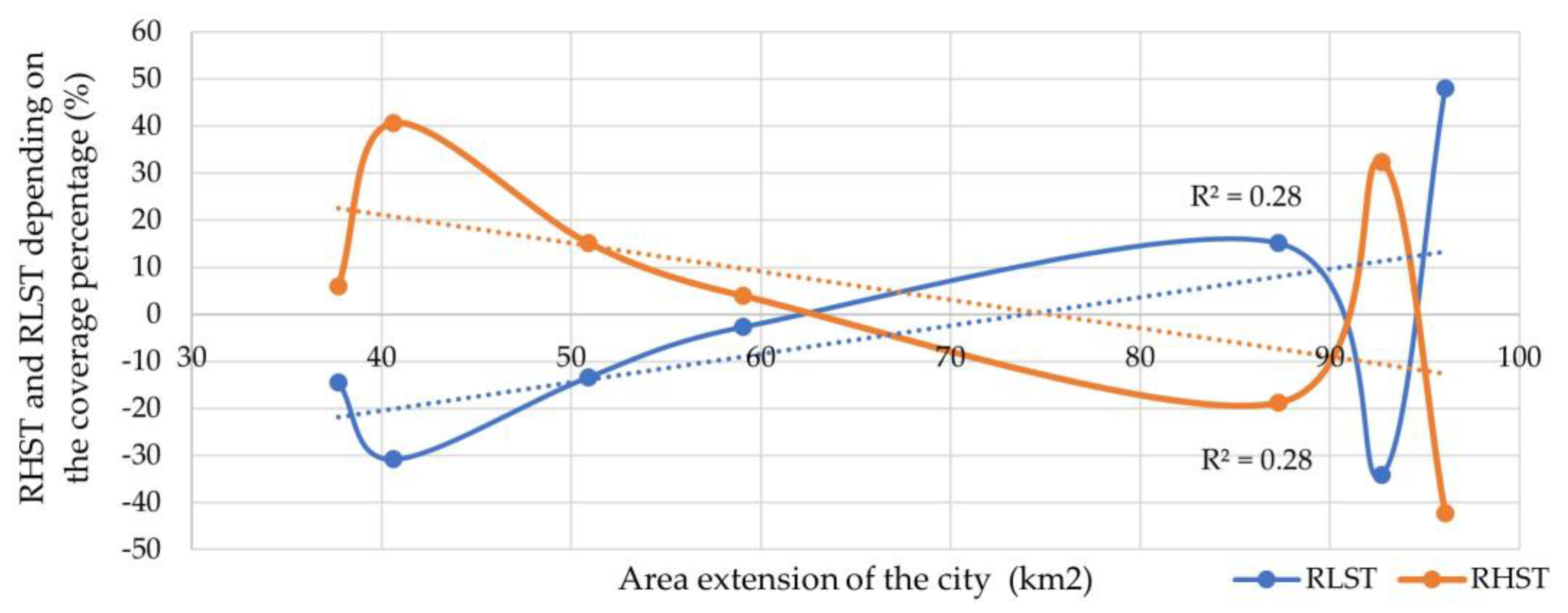
Area or extension in km2	0.28	0.28
Number of inhabitants	0.21	0.31
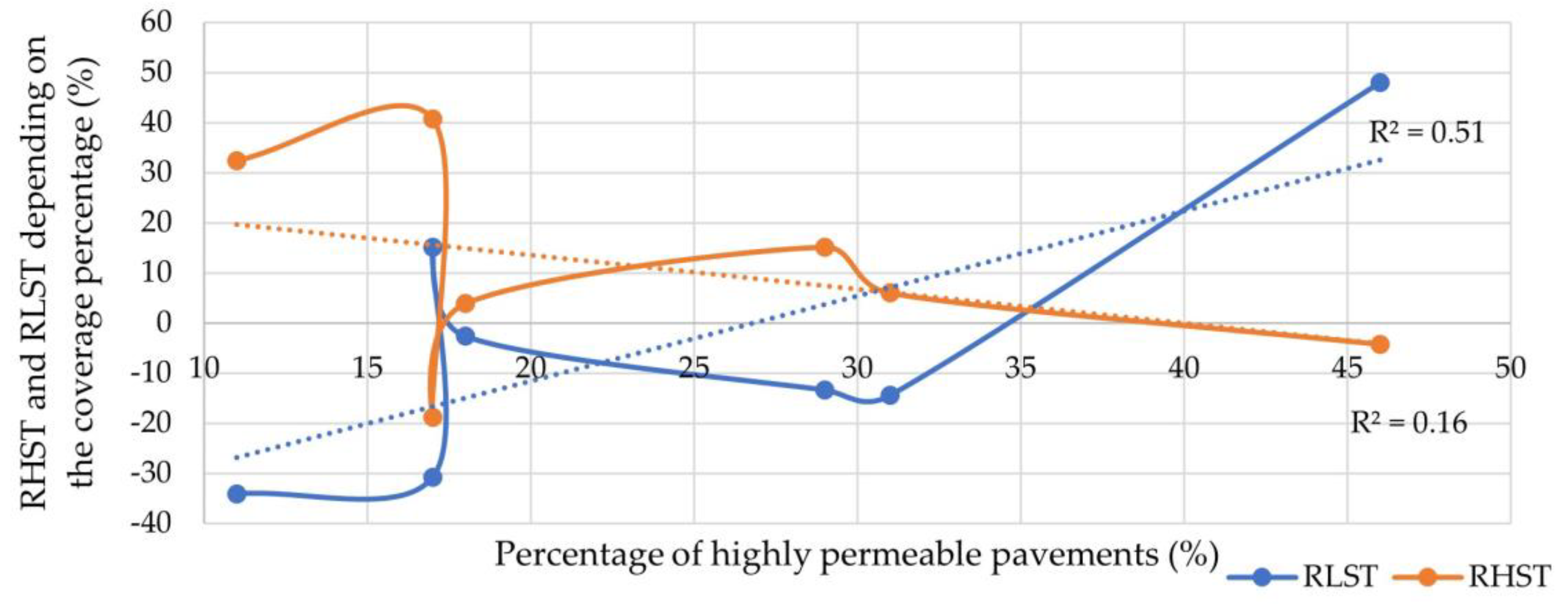
Highly impermeable pavements	0.16	0.51
Moderately impermeable pavements	0.07	0.05
Slightly impermeability pavements	0.14	0.19
High NDVI	0.34	0.32
Low NDVI	0.22	0.01

is derived from the values presented in the graphs in Figure 12, Figure 13, Figure 14, Figure 15, Figure 16, Figure 17 and Figure 18; it highlights the relationships or correlations between them. This table facilitates a discussion of the results, which are further addressed in the conclusions.

Figure 12 illustrates the relationship between the representative low surface temperature (RLST) and the representative high surface temperature (RHST) with the variable of land area, measured in square kilometers (km²). We observe that the trends for the RHST (R² = 0.28) and RLST (R² = 0.28) are similar. Specifically, on the corresponding day in July 2020, the low temperature occupied a larger area, while the high temperature tended to be more contracted.

In the case of Figure 13, which considers the number of inhabitants, the RLST (R² = 0.31) shows an improved correlation compared to the RHST (R² = 0.21). In both cases (land area and population), the graphs exhibit similar behavior.

Regarding highly permeable soils (Figure 14), moderately permeable soils (Figure 15), and poorly permeable soils (Figure 16), the best correlation was observed for RLST in highly permeable soils, with R² = 0.51. Moderately permeable soils showed the weakest correlation, while poorly permeable soils exhibited similar correlation values for the RHST (R² = 0.14) and RLST (R² = 0.19).

The high NDVI (Figure 17) values indicated that the RLST (R² = 0.32) and RHST (R² = 0.34) exhibit an inverse trend; however, both show similar correlation levels. Considering all cases, the low NDVI (Figure 18) was the least strongly correlated with the variable of mobility, where the RLST obtained a value of R² = 0.01.

Figure 19 shows the average of all temperatures recorded on the two days in July 2019 and 2020 as an indicator of overall trends.

5. Conclusions

This research enabled a comparison between two selected days in seven cities with similar meteorological conditions. The key factor was that the day corresponding to July 2020 exhibited a mobility decrease of over 40% compared to its July 2019 counterpart; this was because of the quarantine and social distancing measures implemented due to COVID-19.

Figure 19 shows that three cities experienced a decrease in their average temperature of approximately 5 °C, while four cities exhibited an upward trend, with two presenting a difference between 4 and 6 °C and the other two between 0.1 and 0.6 °C.

The variables of land area and population size (Figure 12 and Figure 13), in addition to showing similar correlation values ranging in 0.28, indicate that mobility affects thermal behavior. Furthermore, the RHST and RLST are inversely proportional, meaning that, while the RLST tends to increase, the RHST tends to decrease.

Considering all values, we can deduce that, for highly impermeable soils, the RLST had the best correlation, whereby a larger area of this soil type leads to low temperatures occupying more area in the city when mobility decreases. However, the RHST is not directly proportional (R² = 0.15). In the cases of moderately and poorly impermeable soils, the RHST tended to increase when mobility decreased, while the RLST occupied a smaller area in the city.

The vegetation index was a key determinant of temperatures within a city [55,56,57]. The higher the vegetation index, the more the RHST decreases, and the RLST equalizes in the same proportion. This pattern was also observed, albeit to a lesser extent, in areas with a low NDVI, where the RLST had the lowest value.

The study found that cities with elongated shapes, such as Manzanillo and Ciudad del Carmen, showed a similar pattern between the two examined days, which is also reflected in their relatively consistent NDVI values. In contrast, more centralized cities experienced significant changes in their surface temperatures between the two days, with specific thermal profiles increasing or decreasing almost equally (Figure 19). Lázaro Cárdenas, Veracruz, and Coatzacoalcos experienced a marked reduction of approximately 5 °C in their average temperatures on the 2020 day, accompanied by a smaller increase in the NDVI.

Conversely, Puerto Vallarta and Tampico exhibited opposite trends, with temperature increases of 4.49 °C and 6.14 °C, respectively, and a corresponding decrease in the NDVI. However, changes in vegetation did not show a direct proportionality with temperature fluctuations, either in terms of increases or decreases. The analysis of thermal images (Figure 4, Figure 5, Figure 6, Figure 7, Figure 8, Figure 9, Figure 10 and Figure 11) revealed that the regions with the highest surface temperatures, except for Ciudad del Carmen, were primarily designated for industrial, port, or transportation functions rather than residential use. Despite a reduction in industrial activity during 2020, it remained a significant factor.

The analysis of the thermal maps of the Pacific Ocean cities allowed for the identification of the following patterns. In Puerto Vallarta, the Gustavo Díaz Ordaz International Airport consistently presented the highest isotherm, in contrast with the nearby natural protected area of “El Salado.” Manzanillo exhibited stable high isotherms at Federal Electricity Commission (CFE) complex and the National Commission of Mexican Petroleum (PEMEX) pelletizing plant, with a certain isothermal territorial extension at the CFE thermoelectric plant. Lázaro Cárdenas experienced declines in temperature; however, the port and PEMEX complexes maintained the highest points in both years.

Within the Gulf of Mexico, the Madero refinery in Tampico and the adjacent port complex exhibited a more pronounced LST, with a decreasing isothermal extension near the refinery but a greater extension within residential areas. Veracruz showed highlights around the Bruno Pagliai Industrial Zone and the port area. Despite a similar temperature curve behavior in Coatzacoalcos, there was a general expansion, rather than an increase in temperature, throughout the city, with the “Pajaritos” petrochemical complex consistently having the highest temperature readings. In Ciudad del Carmen, the isothermal patterns remained constant over two years, with peaks observed at the international airport and two concrete parking structures adjacent to shopping centers.

These findings, based on the analysis of seven cities, enhance our understanding of how mobility affects various factors that influence the thermal behavior of urban surfaces. Although a temporary phenomenon that arose during confinement, the changes in LST due to mobility provide us with an opportunity to investigate how factors such as land area, population size, types of impermeable soils, and the NDVI were modified, presenting exploratory and correlational research that paves the way for the future implementation of policies related to mobility, which might improve the thermal comfort level of citizens.

This is an area with research potential. It is recognized that, although there are few data points that have a conclusive statistical correlation, this study only seeks to perform an exploratory analysis and a comparison of two days, since the second of these dates fell during the peak of social distancing due to COVID-19, which modified urban mobility. The article opens up a discussion of how mobility affects the LST, associated with SUHI, setting a precedent for future research and analysis.

References

- Li, H.; Zhou, Y.; Li, X.; Meng, L.; Wang, X.; Wu, S.; Sodoudi, S. A new method to quantify surface urban heat island intensity. Sci. Total Environ. 2018, 624, 262–272. [Google Scholar] [CrossRef]
- Parsaee, M.; Joybari, M.M.; Mirzaei, P.A.; Haghighat, F. Urban heat island, urban climate maps and urban development policies and action plans. Environ. Technol. Innov. 2019, 14, 100341. [Google Scholar] [CrossRef]
- Peng, S.; Piao, S.; Ciais, P.; Friedlingstein, P.; Ottle, C.; Bréon, F.-M.; Nan, H.; Zhou, L.; Myneni, R.B. Surface urban heat island across 419 global big cities. Environ. Sci. Technol. 2012, 46, 696–703. [Google Scholar] [CrossRef]
- Kuttler, W.; Weber, S. Characteristics and phenomena of the urban climate. Meteorol. Z. 2023, 32, 15–47. [Google Scholar] [CrossRef]
- Hu, Y.; Hou, M.; Jia, G.; Zhao, C.; Zhen, X.; Xu, Y. Comparison of surface and canopy urban heat islands within megacities of eastern China. ISPRS J. Photogramm. Remote Sens. 2019, 156, 160–168. [Google Scholar] [CrossRef]
- Hung, T.; Uchihama, D.; Ochi, S.; Yasuoka, Y. Assessment with satellite data of the urban heat island effects in Asian mega cities. Int. J. Appl. Earth Obs. Geoinf. 2006, 8, 34–48. [Google Scholar]
- JSobrino, J.A.; Irakulis, I. A Methodology for Comparing the Surface Urban Heat Island in Selected Urban Agglomerations Around the World from Sentinel-3 SLSTR Data. Remote Sens. 2020, 12, 2052. [Google Scholar] [CrossRef]
- Lu, L.; Weng, Q.; Xiao, D.; Guo, H.; Li, Q.; Hui, W. Spatiotemporal variation of surface urban heat islands in relation to land cover composition and configuration: A multi-scale case study of Xi’an, China. Remote Sens. 2020, 12, 2713. [Google Scholar] [CrossRef]
- Stewart, I.D.; Krayenhoff, E.S.; Voogt, J.A.; Lachapelle, J.A.; Allen, M.A.; Broadbent, A.M. Time Evolution of the Surface Urban Heat Island. Earth’s Futur. 2021, 9, e2021EF002178. [Google Scholar] [CrossRef]
- Louiza, H.; Zéroual, A.; Djamel, H. Impact of the transport on the urban heat island. Int. J. Traffic Transp. Eng. 2015, 5, 252–263. [Google Scholar] [CrossRef] [PubMed]
- Kolbe, K. Mitigating urban heat island effect and carbon dioxide emissions through different mobility concepts: Comparison of conventional vehicles with electric vehicles, hydrogen vehicles and public transportation. Transp. Policy 2019, 80, 1–11. [Google Scholar] [CrossRef]
- Kim, Y.; Yeo, H.; Kim, Y. Estimating urban spatial temperatures considering anthropogenic heat release factors focusing on the mobility characteristics. Sustain. Cities Soc. 2022, 85, 104073. [Google Scholar] [CrossRef]
- Kusak, L.; Kucukali, U.F. Investigating the relationship between COVID-19 shutdown and land surface temperature on the Anatolian side of Istanbul using large architectural impermeable surfaces. Environ. Dev. Sustain. 2021, 26, 18439–18476. [Google Scholar] [CrossRef] [PubMed]
- Parida, B.R.; Bar, S.; Roberts, G.; Mandal, S.P.; Pandey, A.C.; Kumar, M.; Dash, J. Improvement in air quality and its impact on land surface temperature in major urban areas across India during the first lockdown of the pandemic. Environ. Res. 2021, 199, 111280. [Google Scholar] [CrossRef] [PubMed]
- Prusa, J.M.; Segal, M.; Temeyer, B.R.; Gallus, W.A.; Takle, E.S. Conceptual and scaling evaluation of vehicle traffic thermal effects on snow/ice-covered road. J. Appl. Meteorol. Climatol. 2002, 41, 1225–1240. [Google Scholar] [CrossRef]
- Chapman, L.; Thornes, J.E. The influence of traffic on road surface temperatures: Implications for thermal mapping studies. Meteorol. Appl. 2005, 12, 371–380. [Google Scholar] [CrossRef]
- Khalifa, A.; Marchetti, M.; Bouilloud, L.; Martin, E.; Bues, M.; Chancibaut, K. Accounting for anthropic energy flux of traffic in winter urban road surface temperature simulations with the TEB model. Geosci. Model Dev. 2016, 9, 547–565. [Google Scholar] [CrossRef]
- Zhou, B.; Rybski, D.; Kropp, J.P. The role of city size and urban form in the surface urban heat island. Sci. Rep. 2017, 7, 4791. [Google Scholar] [CrossRef]
- Zhou, B.; Rybski, D.; Kropp, J.P. On the statistics of urban heat island intensity. Geophys. Res. Lett. 2013, 40, 5486–5491. [Google Scholar] [CrossRef]
- Arnfield, A. Two decades of urban climate research: A review of turbulence, exchanges of energy and water, and the urban heat island. Int. J. Climatol. A J. R. Meteorol. Soc. 2003, 23, 1–26. [Google Scholar] [CrossRef]
- Zhao, L.; Lee, X.; Smith, R.B.; Oleson, K. Strong contributions of local background climate to urban heat islands. Nature 2014, 511, 216–219. [Google Scholar] [CrossRef] [PubMed]
- Dewan, A.; Kiselev, G.; Botje, D.; Mahmud, G.I.; Bhuian, M.H.; Hassan, Q.K. Surface urban heat island intensity in five major cities of Bangladesh: Patterns, drivers and trends. Sustain. Cities Soc. 2021, 71, 102926. [Google Scholar] [CrossRef]
- Ferrari, A.; Kubilay, A.; Derome, D.; Carmeliet, J. The use of permeable and reflective pavements as a potential strategy for urban heat island mitigation. Urban Clim. 2020, 31, 100534. [Google Scholar] [CrossRef]
- Morabito, M.; Crisci, A.; Guerri, G.; Messeri, A.; Congedo, L.; Munafò, M. Surface urban heat islands in Italian metropolitan cities: Tree cover and impervious surface influences. Sci. Total Environ. 2021, 751, 142334. [Google Scholar] [CrossRef] [PubMed]
- Chun, B.; Guldmann, J.-M. Impact of greening on the urban heat island: Seasonal variations and mitigation strategies. Comput. Environ. Urban Syst. 2018, 71, 165–176. [Google Scholar] [CrossRef]
- Fathizad, H.; Tazeh, M.; Kalantari, S.; Shojaei, S. The investigation of spatiotemporal variations of land surface temperature based on land use changes using NDVI in southwest of Iran. J. Afr. Earth Sci. 2017, 134, 249–256. [Google Scholar] [CrossRef]
- Neinavaz, E.; Skidmore, A.K.; Darvishzadeh, R. Effects of prediction accuracy of the proportion of vegetation cover on land surface emissivity and temperature using the NDVI threshold method. Int. J. Appl. Earth Obs. Geoinf. 2020, 85, 101984. [Google Scholar] [CrossRef]
- Saha, M.; Al Kafy, A.; Bakshi, A.; Abdullah-Al-Faisal; Almulhim, A.I.; Rahaman, Z.A.; Al Rakib, A.; Fattah, M.A.; Akter, K.S.; Rahman, M.T.; et al. Modelling microscale impacts assessment of urban expansion on seasonal surface urban heat island intensity using neural network algorithms. Energy Build. 2022, 275, 112452. [Google Scholar] [CrossRef]
- SCT. Secretari de Comunicaciones y Transportes. 2020. [En Línea]. Available online: http://www.sct.gob.mx/puertos-y-marina/puertos-de-mexico/ (accessed on 18 August 2023).
- INEGI. Espacio y Datos de México. 2020. [En Línea]. Available online: https://www.inegi.org.mx/app/mapa/espacioydatos/ (accessed on 7 September 2023).
- INAFED. Enciclopedia de Los Municipios y Delegaciones de México. 2018. [En Línea]. Available online: http://www.inafed.gob.mx (accessed on 15 October 2021).
- INEGI. Censo de Población y Vivienda. 2020. [En Línea]. Available online: http://cuentame.inegi.org.mx (accessed on 15 October 2021).
- SEDESOL. Unidad de Microrregiones. 2015. [En Línea]. Available online: http://www.microrregiones.gob.mx (accessed on 13 October 2021).
- Gobierno del Estado de Tamaulipas. Tampico. 2016. [En Línea]. Available online: https://www.tamaulipas.gob.mx/estado/municipios/tampico/ (accessed on 15 October 2021).
- IMEPLAN. Programa Metropolitano de Ordenamiento Territorial de Altamira-Ciudad Madero-Tampico; IMEPLAN: Zapopan, Mexico, 2019. [Google Scholar]
- Gobierno de Mexico. Comisión Nacional del Agua. 21 August 2022. [En Línea]. Available online: https://smn.conagua.gob.mx/es/informacion-climatologica-por-estado?estado=df (accessed on 14 October 2023).
- Peel, M.C.; Finlayson, B.L.; McMahon, T.A. Updated world map of the Köppen-Geiger climate classification. Hydrol. Earth Syst. Sci. 2007, 11, 1633–1644. [Google Scholar] [CrossRef]
- Martin, S.; Bergmann, J. (Im)mobility in the Age of COVID-19. Int. Migr. Rev. 2021, 55, 660–687. [Google Scholar] [CrossRef]
- Conahcyt. Conahcyt Frente a la COVID-19. 25 April 2022. [En Línea]. Available online: https://salud.conacyt.mx/coronavirus/investigacion/proyectos/movilidad.html (accessed on 19 November 2023).
- Anderson, M.C.; Kustas, W.P.; Norman, J.M.; Hain, C.R.; Mecikalski, J.R.; Schultz, L.; González-Dugo, M.P.; Cammalleri, C.; d’Urso, G.; Pimstein, A.; et al. Mapping daily evapotranspiration at field to continental scales using geostationary and polar orbiting satellite imagery. Hydrol. Earth Syst. Sci. 2011, 15, 223–239. [Google Scholar] [CrossRef]
- Rosado, R.M.G.; Guzmán, E.M.A.; Lopez, C.J.E.; Molina, W.M.; García, H.L.C.; Yedra, E.L. Mapping the LST (Land Surface Temperature) with Satellite Information and Software ArcGis. IOP Conf. Ser. Mater. Sci. Eng. 2020, 81, 012045. [Google Scholar] [CrossRef]
- García-Santos, V.; Cuxart, J.; Martínez-Villagrasa, D.; Jiménez, M.A.; Simó, G. Comparison of three methods for estimating land surface temperature from landsat 8-tirs sensor data. Remote Sens. 2018, 10, 1450. [Google Scholar] [CrossRef]
- Sekertekin, A. Validation of physical radiative transfer equation-based land surface temperature using Landsat 8 satellite imagery and SURFRAD in-situ measurements. J. Atmos. Sol.-Terr. Phys. 2019, 196, 105161. [Google Scholar] [CrossRef]
- Vanhellemont, Q. Combined land surface emissivity and temperature estimation from Landsat 8 OLI and TIRS. ISPRS J. Photogramm. Remote Sens. 2020, 166, 390–402. [Google Scholar] [CrossRef]
- de la Rubia, E.A. Caracterización de la isla de calor urbana en el campus de la UAM por medio de teledetección. Geofocus Rev. Int. Cienc. Y Tecnol. La Inf. Geográfica 2020, 26, 4. [Google Scholar]
- Buo, I.; Sagris, V.; Uuemaa, I.B.Y.E. Estimating the expansion of urban areas and urban heat islands (UHI) in Ghana: A case study. Nat. Hazards 2021, 105, 1299–1321. [Google Scholar] [CrossRef]
- Dijoo, Z.K. Urban Heat Island Effect Concept and Its Assessment Using Satellite-Based Remote Sensing Data. In De Geographic Information Science for Land Resource Management; Scrivener Publishing LLC: Beverly, MA, USA, 2021; pp. 81–98. [Google Scholar]
- Gartland, L.M. Heat Islands: Understanding and Mitigating Heat in Urban Areas; Francis, T., Ed.; Routledge: New York, NY, USA, 2012. [Google Scholar]
- Oke, T. The urban energy balance. Prog. Phys. Geogr. 1988, 12, 471–508. [Google Scholar] [CrossRef]
- Martín-Morales, G. Protocolo Para la Obtención de la Temperatura de la Superficie Terrestre a Partir de Datos LandSat y Modis; Instituto de Geografía Tropical: La Habana, Cuba, 2015. [Google Scholar]
- Acharya, T.D.; Yang, I. Exploring landsat 8. Int. J. IT Eng. Appl. Sci. Res. 2015, 4, 4–10. [Google Scholar]
- Palacios-Sánchez, L.; Paz-Pellat, F.; Oropeza-Mota, J.; Figueroa-Sandoval, B.; Martínez-Menez, M.; Ortiz-Solorio, C.; Exebio-García, A. Corrector atmosférico en imágenes Landsat. Tierra Latinoam. 2018, 36, 309–321. [Google Scholar]
- Salinas-Zavala, C.A.; Martínez-Rincón, R.O.; Morales-Zárate, M.V. Tendencia en el siglo XXI del Índice de Diferencias Normalizadas de Vegetación (NDVI) en la parte sur de la península de Baja California. Investig. Geográficas Boletín Del Intituto De Geogr. 2017, 94, 82–90. [Google Scholar] [CrossRef]
- Najafzadeh, F.; Mohammadzadeh, A.; Ghorbanian, A.; Jamali, S. Spatial and temporal analysis of surface urban heat island and thermal comfort using landsat satellite images between 1989 and 2019: A case study in Tehran. Remote Sens. 2021, 13, 4469. [Google Scholar] [CrossRef]
- Xiao, X.D.; Dong, L.; Yan, H.; Yang, N.; Xiong, Y. The influence of the spatial characteristics of urban green space on the urban heat island effect in Suzhou Industrial Park. Sustain. Cities Soc. 2018, 40, 428–439. [Google Scholar] [CrossRef]
- Maheng, D.; Ducton, I.; Lauwaet, D.; Zevenbergen, C.; Pathirana, A. The Sensitivity of Urban Heat Island to Urban Green Space—A Model-Based Study of City of Colombo, Sri Lanka. Atmosphere 2019, 10, 151. [Google Scholar] [CrossRef]
- Arghavani, S.; Malakooti, H.; Bidokhti, A.-A.A.A. Numerical assessment of the urban green space scenarios on urban heat island and thermal comfort level in Tehran Metropolis. J. Clean. Prod. 2020, 261, 121183. [Google Scholar] [CrossRef]