On-Site Sensor Sensitivity Adjustment Technique for a Maintenance-Free Heat Flow Monitoring in Building Systems

Abstract

In this paper, an advanced solution for measuring heat flow through opaque building elements is presented. The solution is based on the implementation of a computer-aided technique for continuous monitoring of heat flow sensor performance and silent checking of their accuracy. In principle, the technique provides an ex-post compensation of potential deviations and inaccuracies detected during the measurement, which can be done without interfering with the ongoing experiment. As a consequence, traditional ‘non-smart’ sensors can be turned into advanced sensors with self-sensing or self-adjustment features at nearly zero additional costs. The high efficiency of the proposed approach was validated against experimental data obtained from an independent set of advanced high-sensitive sensors. Considering the validation results, the proposed technique brings an entirely new potential for maintenance-free applications for thermal performance monitoring in the building sector, typically for long-term experiments or measurements under dynamic environments.

1. Introduction

In the thermal assessment of buildings, various types of heat gains and losses constitute the overall balance of the object. Its character, whether positive or negative, depends mostly on the thermal performance of the building enclosure [1,2]. Therefore, the heat transfer analysis of this building element should receive special attention to provide an essential part of the data that forms a considerable contribution to the overall heat balance of buildings.

Heat flux probes and sensors considered for applications in the building sector need to meet specific requirements, such as relatively low values of heat flux, alternating directions of heat flux, surface roughness of investigated walls, or exposure to radiative heat flux. Various types of sensors are available on the market, differing from each other by measuring techniques and/or construction principles. Gardon [3,4,5], Schmidt-Boelter gauges [6,7,8], thin plate sensors [9,10], or radiometers [11,12] represent the most common types of non-optical sensors. An extensive review of heat flux measuring techniques was provided by Childs et al. [13]. Another report [14] provided a review of non-optical detectors for heat flux measurement in fires. Assuming that heat flux can be induced by different origins, the essential criterion of sensor selection should be made with respect to the environment, in which the sensor is intended to be placed in. Basically, the heat flux mode or possible combination of multiple modes (convective, radiative, or conductive), including the range of anticipated quantities, should be known in advance to provide a background for making a qualified decision on sensor selection. For example, Gardon and Schmidt-Boelter gauges were designed for the measurement of both convective and radiative heat fluxes. As such, they are suitable for fire- or flame-induced heat transfer measurement. Pure radiative transfer, such as solar radiation, can be measured by pyranometers [15]. The conductive heat transfer is typical for building physics applications in the case that opaque building elements are the subject of investigation. As the sensors are mostly mounted on the wall surface, flat plate sensors or foil sensors suit best for these kind of applications. Those sensors are represented by thermopiles working on the principle of the Seebeck effect; that is, they generate an electrical output signal that is proportional to the heat flux passing through the sensor. Before application, each transducer needs to be calibrated to determine its sensitivity, that is, the electrical output to the passing heat flux ratio. In most cases, the initial calibration is performed by the manufacturer and the user is provided with the calibration protocol. Also, the default sensitivity is very often printed somewhere on the sensor body to be easily located and adopted by the user.

The common practice for the calibration of heat flux transducers is based on inducing steady-state conductive heat flux in the controlled environment by means of the guarded hot plate [16] or the heat flow meter apparatus [17,18]. Procedures for calibrating heat flux probes that are relatively thin in comparison with their planar dimensions are well described in ASTM C1130 [19]. This practice in conjunction with other test methods serves as a valuable handbook for the determination of the sensitivity of heat flux transducers under both laboratory and in-situ conditions.

For the laboratory calibration, the conjunction with Test Methods C177 [16], C518 [17], C1363 [20], C1114 [21], or ISO 8302 [22] is well appreciated, while three different techniques are recognized: (i) ideally-guarded, (ii) embedded, and (iii) surface mounted. As described in Section 4.1 of ASTM C1130 [19], the ideally protected technique (i) is used for determining the baseline calibration assuming that only homogeneous and thermally characterized materials are used in the test stack (series of layers) promoting one-dimensional heat flow. The (ii) embedded technique is based on the same principle as (i); however, material layers identical or comparable to the building construction to be studied under application are used, instead. The surface-mounted calibration technique (iii) represents the most complex approach as it needs to address and incorporate all environmental effects that may cause the lateral heat flow in the vicinity of the applied sensor.

The conjunction of ASTM C1130 with C1046 [23] allows the calibration results to be used for in situ measurement of heat flux through opaque building elements with subsequent analysis of measurement data according to ASTM C1155 [24]. The in-situ measurement practice provides practical information, recommendations, and tips to ensure potential simplicity and ease of application of heat flux sensors. A comprehensive study to support the continuous development of precision and bias statements for ASTM Practice C 1130 was published by Zarr et al. [25], in which the authors provided a complex analysis of common issues that are typical for building applications. In that study, sensor equivalency, linearity and temperature effects, uncertainty analysis, and suitability test method were analyzed, which can partially address some of the typical issues associated with heat flux measurements in the building sector. According to the practice [19], the heat flux transducer that is to be mounted on the building envelope construction should be calibrated using a hot box that is oriented similarly to the measuring site. Additionally, this approach requires a specific configuration and sample preparation involving a homogeneous specimen of known thermal resistance, temperature sensor, and guarded mask to obtain reliable results. Also, the calibration should be performed at levels of temperature and relative humidity consistent with the end-use conditions.

Varying conditions during in-situ measurement may bring significant uncertainties to the measurement, therefore periodic performance checks should be carried out to reflect those fluctuations and to minimize measurement errors. However, such checks, according to the above-described practices, require unmounting the sensor thus interfering with the ongoing experiment. Some initiatives to address the varying sensitivity has come directly from the sensor producers, which documents the awareness of this issue. This initiative resulted in the introduction of new commercial gauges that were capable of self-calibration without the need for sensor removal in certain applications [26,27]. The advanced solution is based on a novel design of the sensors with integrated heaters in sensor bodies to generate a controlled heat flux allowing a subsequent auto-calibration. Moreover, it is worth mentioning that some of the heat flux plates for measurement in buildings were originally developed for meteorological applications to measure heat fluxes in soils, which predetermines the self-calibration practice. Such practice presumes that the sensor is surrounded by soil during measurement. Typically, when the built-in heater is activated to generate the prescribed heat flux, the surrounding soil with equal properties ensures that half of the flux will be transferred upwards, while the other half will go downwards. This is an essential assumption for sensor calibration [28]. If the advanced sensors are mounted on the wall, surface-specific conditions must be ensured, similar to those in laboratory calibration using ASTM practices. This can bring some serious limitations or drawbacks or even exclude the in-situ self-calibrations of advanced sensors in the building sector.

An alternative to the standard calibration procedures might be represented by the approach proposed in this paper, which turns the traditional sensors applied in the building sector into advanced ones. The approach allows for the continuous measure of the heat flow without a need to interfere with the ongoing experiment. Moreover, the heat flux sensor may even stay mounted on the wall surface providing the edge over advanced sensors with integrated heaters and turning the non-smart sensors into smart ones. The term “smart” refers to the capability of the proposed method to effectively substitute the heat source element that is present in the standard calibration procedure at any time without extending or upgrading the experimental apparatus. The conjunction of experimental and computational methods used in the proposed approach makes it possible to accommodate specific requirements of the calibration procedure and facilitate various applications of the sensors in heat flux analyses in the building sector. As such it can contribute to the state-of-the-art and extend the numerical methods for the in-situ data analysis as mentioned in [19]. To demonstrate the capability of the proposed method, a “free-running” residential building with varying indoor environments was selected for long-term monitoring of environmental variables and wall performance. Then, the experimental data were analyzed and complemented with the outputs of a computational analysis to reveal potential deviations in the sensor performance using the ex-post scheme. If some deviation was detected then the complex experimental-computational datasets allowed for a compensation of errors resulting from the varying sensitivity of the probes, thus, consistently ensuring a high level of accuracy of heat flux measurement with a standard “non-smart” experimental equipment. This could be achieved by recording and analyzing both raw sensor data and end-user outputs in the form of heat flux variations. To validate the findings presented in this paper, the experimental setup was extended in the final stage of the field monitoring by the acquisition of high-sensitive flat plate sensors with the film heater integrated into the sensor body. Such a configuration allowed the proposed technique to be directly compared against the independent data, which is the essential precondition for performing the independent validation.

2. Materials and Methods

2.1. Theoretical Background

A one-dimensional problem is considered for the analysis of transient heat flux on the interior surface of a building wall (see Figure 1), where q_IN represents the rate of heat transfer per unit area, i.e., the heat flux, from the interior to the surface element, q_OUT represents the heat flux from the surface element to the wall, and x is the thickness of wall element.

Assuming that thickness of the element is infinitesimally small, i.e., x → 0, then thermal storage in the element can be practically neglected implying that

q_IN ≈ q_OUT,

(1)

at any time. In Equation (1), q_IN (W·m⁻²) is the heat flux from the interior to the wall surface, q_OUT (W·m⁻²) is the heat flux from the wall surface to the wall. For this case, q_IN can be expressed using the Newton’s law of cooling as

q_IN = α (T_s − T_i),

(2)

where α (W·m⁻²·K⁻¹) is the heat transfer coefficient, T_i (°C) is the ambient wall (indoor) temperature, and T_s (°C) is the interior surface temperature of the wall. The heat flux from the surface element to the wall, q_OUT, can be expressed using Fourier’s equation as

q_OUT = λ ΔT/Δx,

(3)

where λ (W m⁻¹ K⁻¹) is the thermal conductivity, ΔT (°C) is the temperature difference of the element surfaces in the direction of the heat flow, Δx (m) is the thickness of the element in the main direction of the heat flux. When a validated computational model is integrated then the heat transport in the surface element can be included to define a new computational-experimental domain allowing for a complex analysis, which might help to extend the current methods or design new principles for heat flux measurement and building performance simulations.

For the computational modeling of heat transfer, which can provide thermal performance data of the wall to form a complex dataset for the performance check procedure, the modified Künzel’s model of heat and moisture transport was used [29,30]. This model was developed for applications in building engineering and validated several times in the past [31]. A detailed information on the modifications of the original Künzel’s model [32] was given in [30]. The following equations were used to govern the heat and moisture transport:

$${\displaystyle \frac{dH}{dT}}{\displaystyle \frac{\partial T}{\partial t}}=\mathrm{div}\left(\lambda \mathrm{grad}T\right)+L_v\mathrm{div}\left({\delta }_p\mathrm{grad}{p}_v\right),$$

(4)

$$\left[{\rho }_{\mathrm{w}}{\displaystyle \frac{\mathrm{d}w}{\mathrm{d}{p}_{\mathrm{v}}}}+\left(\psi -w\right){\displaystyle \frac{M}{RT}}\right]{\displaystyle \frac{\partial p_{\mathrm{v}}}{\partial t}}=\mathrm{div}\left[D_{\mathrm{g}}\mathrm{grad}{p}_{\mathrm{v}}\right],$$

(5)

where H (J·m⁻³) is the enthalpy density, T (K) is the absolute temperature, t (s) is the time, D_g (s) is the global moisture transport function, L_v (J·kg⁻¹) is the latent heat of evaporation of water, δ_p (s) is the water vapor diffusion permeability, M (kg·mol⁻¹) is the molar mass of water vapor, p_v (Pa) is the partial pressure of water vapor in the porous space, w (m³·m⁻³) is the moisture content by volume, ρ_w (kg·m⁻³) is the density of water, ψ (–) is the total open porosity, and R (J·K⁻¹·mol⁻¹) is the universal gas constant. More details and insights into model formulation and parameter description can be found in [30]. Involving moisture transport in the computational modeling was motivated by the effort to increase the calculation accuracy, particularly to obtain thermal conductivity λ as a moisture-dependent variable λ = λ(w). The indoor boundary conditions for temperature and relative humidity were obtained from the experimental data, as well as outdoor boundary conditions that were defined using outdoor climatic data. The material properties were adopted from the previous research [33,34] and from the material database maintained by the Department of Materials Engineering and Chemistry, Faculty of Civil Engineering, Czech Technical University in Prague.

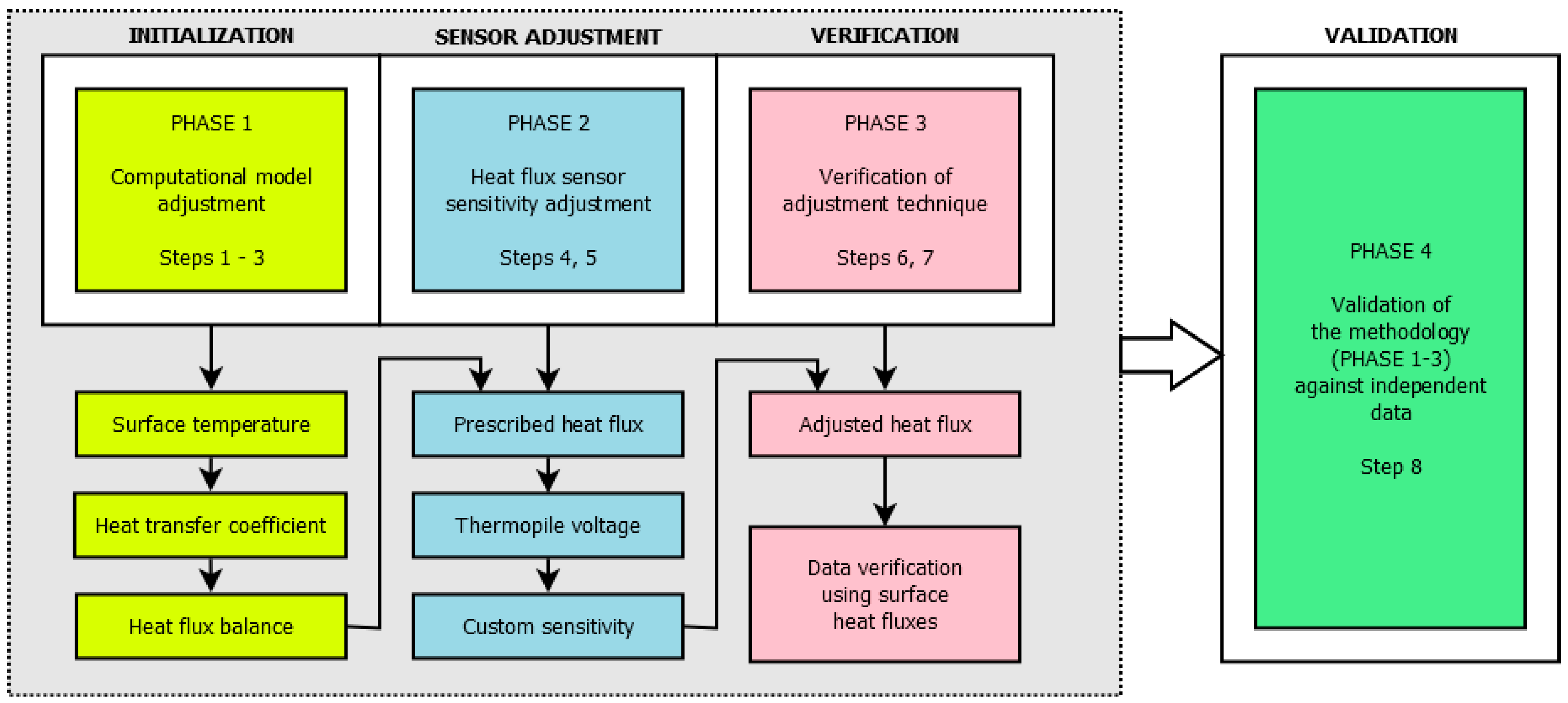
2.2. Design of the Adaptive Self-Adjustment Procedure

The sensitivity adjustment procedure was based on a complex analysis of time-resolved heat fluxes q_IN(t) and q_OUT(t) obtained by both experimental measurements and computational simulation of heat transfer in a studied wall. In the computational simulation, the material composition and orientation of the wall, material properties, and outdoor and indoor environmental data were used as input parameters. At first, the optimization of the computational model parameters was done to validate the capability of the model to simulate the real environment in this particular case. The computational model was optimized by a simple modification of the heat transfer coefficient α on the interior surface of the wall, in order to obtain verified q_IN(t) and q_OUT(t) data through the surface temperature T_s. For this purpose, a surface element with very low thickness (x = 1~2 mm) was used in spatial discretization of the computational model to meet preconditions set in Equation (1). The complex sensitivity adjustment experiment was designed using the following steps:

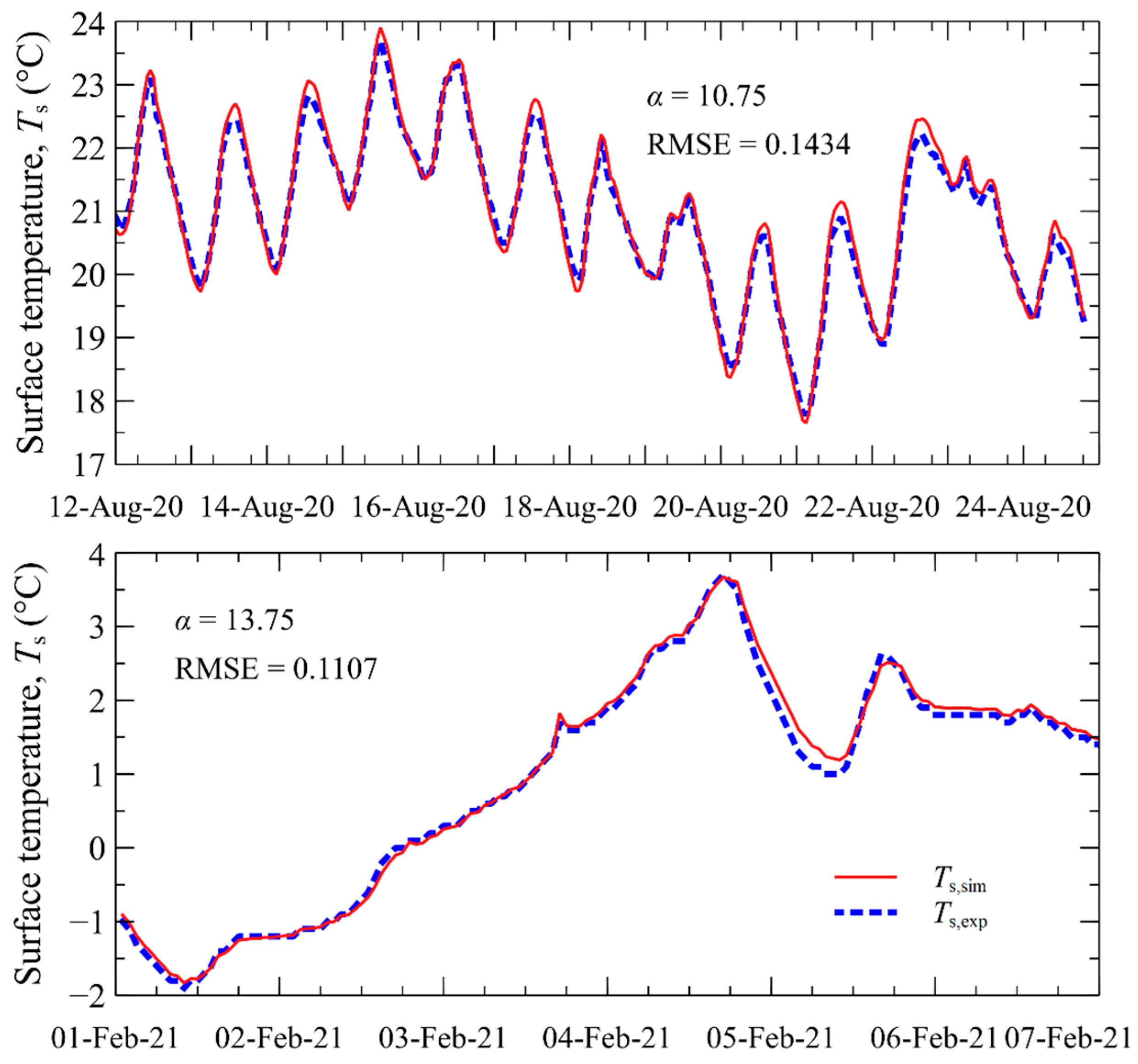
• Heat transfer coefficient α of the computational model is optimized by fitting the simulated surface temperature, T_s,sim(t), to that determined experimentally, T_s,exp (t);
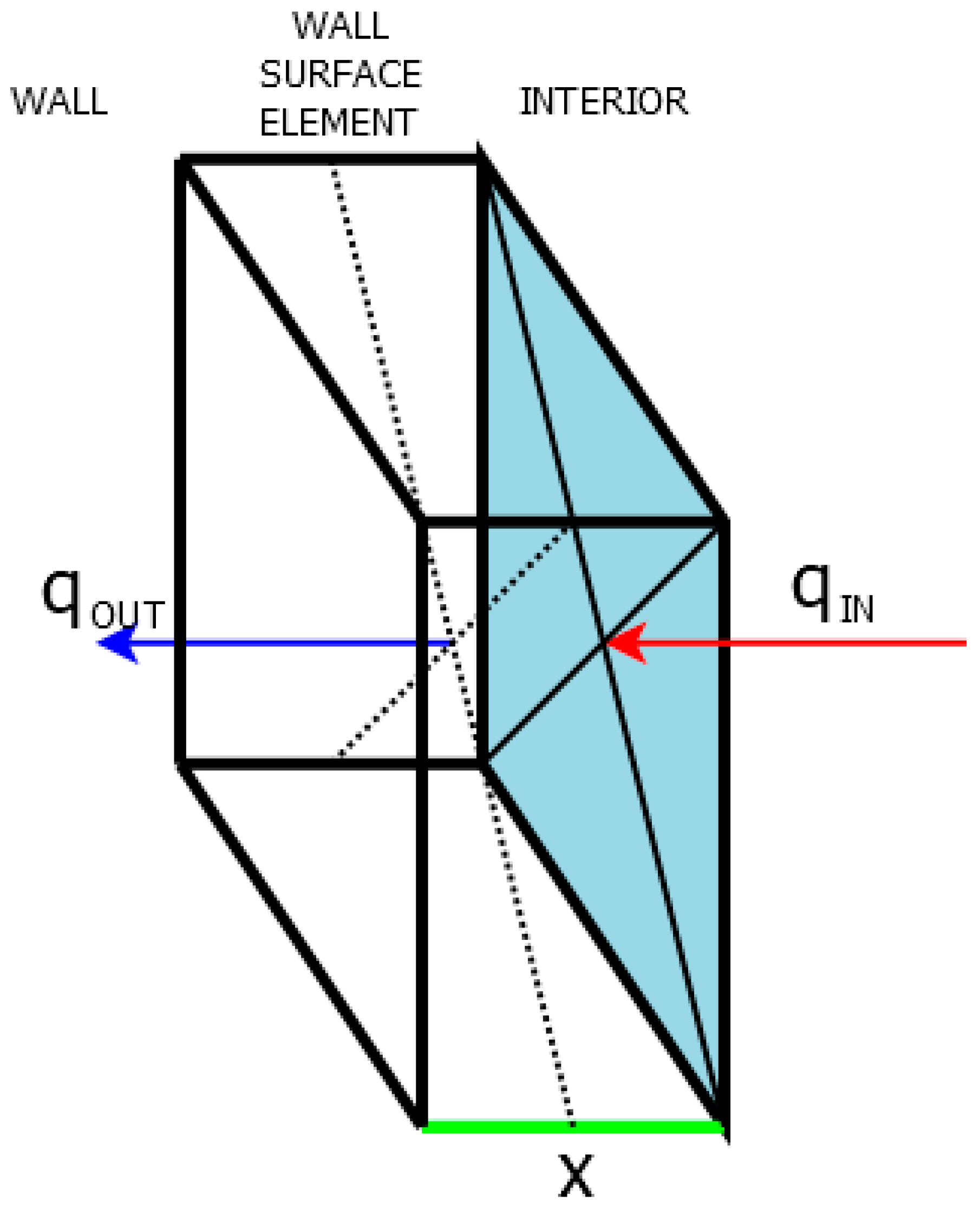
• Heat flux from the interior to the wall surface, q_IN(t), is calculated from the experimental data using Equation (2) and the optimized heat transfer coefficient α from the previous step;
• Heat flux from the wall surface element to the wall, q_OUT(t), is calculated from the computational data using Equation (3) and compared with q_IN(t) from the previous step to validate the setup and accuracy of the computational model;
• q_IN(t) and q_OUT(t) are averaged to form a new variable, q_REF(t), having a sufficient robustness as it combines both experimental and computational outputs;
• Sensitivity of heat flux sensors (thermopiles) is adjusted using raw U(t) (voltage) data and q(t) from the previous step and custom sensitivity function S is identified for each thermopile;
• Raw data provided by the heat flux sensors in the period are adopted and transformed into heat flux using S function from the previous step;
• The heat flux obtained in the previous step is compared with experimentally and computationally derived data to verify the adjusted sensitivity;
• The verified heat flux obtained in the previous step is validated against the reference heat flux obtained from an independent sensor.

The scheme of the designed approach is shown in Figure 2. In general, the experimental measurements can be divided into three phases that correspond to the purposes of data acquisition, processing, and application. The entire procedure can be applied repeatedly during ongoing experiments, providing a tool for an adaptive adjustment which is most effective in the scenarios with changing environmental conditions. The execution of Phase 1 is required to be carried out at least once upon the beginning of the adjusting procedure. Repeated executions of this phase are optional. However, they should be done always when environmental conditions significantly deviate from those acting during the last execution. After initialization of the adjustment procedure, the Phase 2 is carried out to obtain updated sensitivity of the heat flux sensor that will correspond with the actual environmental conditions. With the sensitivity adjusted in this way, the experiment may continue running while Phase 3 is being continuously executed in the background to verify the performance of the heat flux sensor. If some deviation is detected, i.e., substantial difference between measured heat flux and q(t) calculated from the computational model and observed quantities, a repeated execution of Phase 2 and 3 is desired. Phase 4, which represents the independent validation of the proposed technique, is executed for the scientific purposes in this paper only, in order to confirm the applicability of the proposed method. Once the validation is successfully completed, it can stay outside the self-adjustment procedure in practical applications. More details of the validation procedure will be given in the further sections of this paper.

The ability of the smart adjustment approach to respond quickly to changing conditions does not place strict demands on the robustness of training data. Therefore, smaller datasets can be selected for the computational model initial setup and sensor sensitivity re-adjustment. Moreover, the scheme of the proposed method allows the initialization phase (Phase 1) to be executed on the same datasets as used for sensor adjustment (Phase 2). This would ensure that high accuracy of input data needed for the sensor sensitivity adjustment itself will be kept during the ongoing experiment without a significant increase of time required for calibration. The timing of individual adjustment periods may be driven either by the rate of changes of the ambient environment, monitoring of selected experimental conditions, or the accuracy of the heat flux sensor; they can also be scheduled regularly in user-defined periods. The smart approach thus brings an entirely new potential for maintenance-free applications, which can be fully automated upon the implementation of decision-making rules.

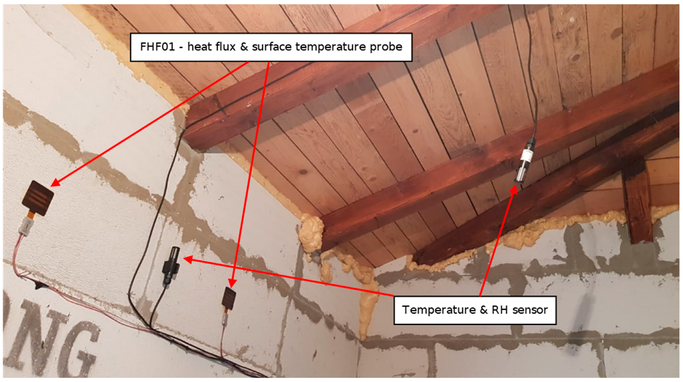
2.3. Self-Adjustment Procedure in Real Conditions

For the demonstration of the proposed technique in real conditions, a residential building in Pulovice (distr. Karlovy Vary), Czech Republic was selected. All necessary data and parameters including climatic variables, structural aspects, material properties, and indoor environmental variables were acquired during that experiment. The summary of data collected within the field survey and experimental measurements is shown in Figure 3.

The realization of the in-situ experiment including a description of the experimental equipment is documented in Figure 4.

The wall was built from autoclaved aerated concrete (AAC) blocks with a thickness of 500 mm which were rendered with a plaster on the exterior surface only. The missing interior render helped to better analyze the background of the heat transport processes in the surface layers as the material characteristics of AAC are known very well and the potential sources of uncertainties could be significantly reduced by a simple visual check. In this way, sources of inhomogeneities or hidden materials in the wall composition could be excluded, which was very appreciating for the adjustment of the computational model. Otherwise, a pre-experimental site inspection using, for example, infrared thermography would be needed as required by C1046 [23].

The outdoor data were collected using the Davis Vanatge Pro2 weather station in 30-min intervals. At the same time resolution, the indoor data were collected using a MS6D Datalogger (by Comet System Ltd., Bratislava, Czech Republic) equipped with two T/RH sensors and two thin-foil heat flux probes Hukseflux FHF01.

Hukseflux sensors are considered thermopiles [35,36], i.e., they consist of a series of thermocouples that measure the temperature difference across the sensor body. The FHF01 is a very thin and flexible foil sensor for general-purpose heat flux measurements equipped with the type T thermocouple to monitor the surface temperature along with the heat flux. The sensor is designed for the measurements of heat flux in the range from −200 to 200 W·m⁻² with a nominal sensitivity of 4.5 × 10⁻⁶ V·m²·W⁻¹

Taking into account specific building-related conditions, such as surface roughness, various types of mountings, and low thermal conductivity of materials, or the conjunction of those factors, the default factory calibration should not always be suitable for heat flux measurement under such conditions. Therefore, a custom sensitivity adjustment approach is presented with the experimental setup described above, which does not require any additional equipment (such as foil heaters) or actions (sensor removal or replacement). Since all probes are classified as thermopiles, i.e., they produce raw data in the form of time-resolved voltage; a user-defined adjustment procedure seems to be optimal to get sufficiently accurate results for each specific application. To guarantee that the overall performance of the building element will be measured, and representative site conditions will be recorded, multiple heat flux sensors were involved in the experimental setup. The summary of input data and parameters that are necessary for both experimental measurement, computational simulation, and in-situ data analysis are shown in

Table 1. Summary of input data used in the simulation and calibration experiment.

	Parameter	AAC	Ext. Plaster
Simulation	ρv (kg·m−3)	500	1244
	ρ (kg·m−3)	2206	2415
	ψ (–)	0.31	0.34
	λ (W·m−1·K−1)	0.12	0.28
	c (J·kg−1·K−1)	1050	1054
	Boundary conditions	Determined experimentally
Experiment	Wall orientation	North
	Wall thickness	500 mm
	Exterior plaster thickness	10 mm

. Here, the following symbols are used: ρ_v (kg·m⁻³) for the bulk density, ρ (kg·m⁻³) for the matrix density (kg·m⁻³), and c (J·kg⁻¹·K⁻¹) is the specific heat capacity.

2.4. Validation of the Proposed Self-Adjustment Approach

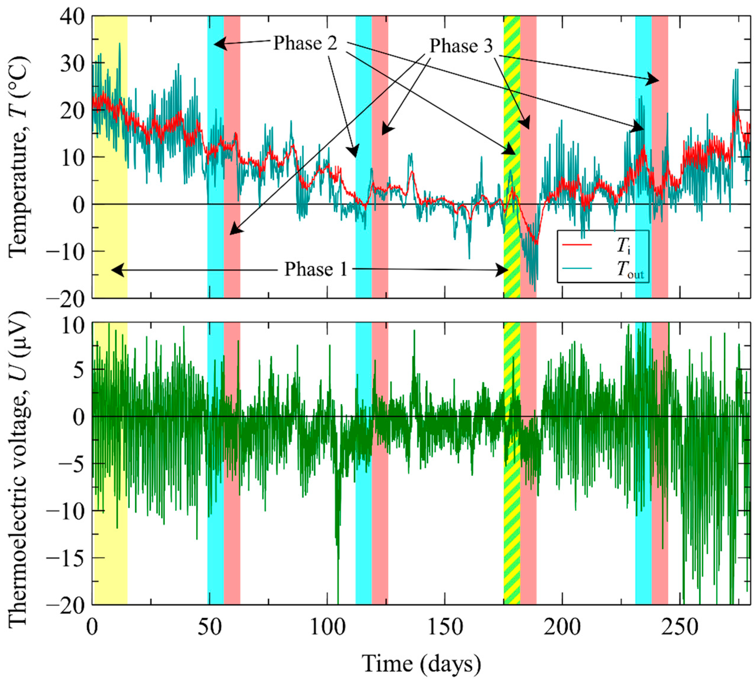
For the independent validation, a series of additional high-sensitive heat flux sensors was acquired and installed on site. In particular, two flat-plate sensors Hukseflux HFP01 and one sensor HFP01SC were mounted on the wall together with the surface temperature sensor Pt1000TG7 (see Figure 5).

HFP01/HFP01SC is a ceramic-plastic composite sensor with a built-in thermopile. The application areas of those sensors include building physics, thermal comfort, or energy budget measurements, as well as geotechnics, meteorology, or other scientific applications based on heat transfer measurement. The sensor is designed for measurements of heat flux in the range from −2000 to 2000 W·m⁻² with a nominal sensitivity of 60 × 10⁻⁶ V·m²·W⁻¹. HFP01SC has identical parameters to HFP01 regarding the heat flux measurement. The only difference between those probes is that HFP01SC contains the film heater to generate prescribed heat flux allowing the sensor to perform self-test and/or self-calibrate.

To prove the efficiency and applicability of the proposed approach, a completely new dataset was obtained using high-sensitive HFP01 and HFP01SC probes in the final stage of the field measurement. Although the sensitivity of HFP sensors is sufficiently high, the HFP01SC was implemented in the measurement to confirm the data obtained by HFP01 during the validation procedure. Having the independent data from those sensitive sensors that stay apart of the sensitivity adjustment procedure described in the previous subsection, the independent validation could be performed by a simple confrontation of the proposed technique with sensor performances. Since the proposed technique potentially aims at the creation of a new alternative to the advanced type of sensors with self-calibration feature, it comes directly from the idea that independent data should be obtained from that kind of sensor. Therefore, additional smart sensors with integrated heaters were acquired, installed on the site, and self-calibrated to provide reference data for the validation.

In principle, the validation is based on a direct comparison of q(t) (obtained using steps 1–4 of the proposed sensor adjustment technique as described in Section 2.3) with the time-resolved reference heat flux (recorded on HFP01 and HFP01SC probes). Although the HFP01 ones are high-sensitive sensors, which is essential for obtaining reliable reference data, the HFP01SC was implemented as well to confirm that reliability through on-site self-calibration. Such self-calibration applied to sensors with integrated heaters is based on measuring the difference in voltage output of the sensor before and after the heating period, and the heat flux generated by the heater to determine the new sensitivity. If the sensors need to stay mounted on the wall, the equal distribution of heat flux must be ensured allowing to use same approximation as dedicated for sensors buried in soils. To achieve this, the sensor was temporarily sandwiched by an AAC block, the same as those which the perimeter wall of the residential object was made of. Therefore, a temporary shelf was mounted on the wall and the sandwiching block was placed on top of it and gently pushed against the sensor. The good thermal contact between upper side of the sensor and temporary sandwiching block was achieved by using pressure-sensitive tape and heat sink grease. Also, the thermal conductivities of both wall and AAC block were checked using an ISOMET device to confirm that the thermal properties correspond to each other, so that Equation (6) can be applied directly without any further compensations. Assuming that the electrically generated heat flux is distributed equally to both sides of the sensor (i.e., half of the heat flux passes the sensor), the new sensitivity can be calculated [37] as

$$S_{\mathrm{SC}}={\displaystyle \frac{2U_{\mathrm{SC}}}{q_{\mathrm{SC}}}}={\displaystyle \frac{2U_{\mathrm{SC}}{R^2}_{\mathrm{current}}{A}_{\mathrm{heater}}}{{U^2}_{\mathrm{current}}{R}_{\mathrm{heater}}}},$$

(6)

where S_SC sensor sensitivity obtained using the self-calibration technique (V·W⁻¹·m²), U_SC (V) is the difference in the voltage output of the sensor before and after the heating period during self-calibration, q_SC (W·m⁻²) is the heat flux generated by the integrated heater, R_heater (Ω) is the nominal resistance of the film heater integrated in the heat flux probe, R_current (Ω) is the resistance of the current sensing resistor used for self-calibration, A_heater (m²) is the heating area of the heater integrated in the heat flux sensor body, U_current (V) is the voltage measured to estimate the current passing through the heater. The details and the scheme of the electrical connection of the sensor is given in the product documentation [37]. The values of R_heater, A_heater are provided in the calibration certificate delivered along with the heat flux probe. Typically, the measurement of voltage generated by the sensor is taken at the times of t = 0, 180 and 360 s and U_SC is calculated as

$$U_{\mathrm{SC}}=\left|U_{t=180}-{\displaystyle \frac{\left(U_{t=0}+U_{t=360}\right)}{2}}\right|,$$

(7)

where U (V) is the voltage signal recorded at the thermopile.

3. Results

The results of experimental measurements and their subsequent processing are shown in the following subsections. The presented outputs of the adjustment procedure should help to analyze its performance and draw conclusions and recommendations for the application of the proposed approach. The experimental measurement was carried out between 10 August 2020 (Day 1) and 16 May 2021 (Day 279) and several sequences from this period were selected for the demonstration of applicability of the proposed sensor sensitivity adjustment method. For the validation, new data were obtained between 1 March 2022 (Day 568) and 17 March 2022 (Day 584). The in-situ experimental data and its processing in the sensor adjustment procedure is shown in Figure 6 and summarized in

Table 2. Summary of experimental data used in the calibration.

	Description	Period
Phase 1	Initialization 1	11 August 2020–24 August 2020
	Initialization 2	1 February 2021–7 February 2021
Phase 2	Sensor adjustment 1	28 September 2020–4 October 2020
	Sensor adjustment 2	31 November 2020–6 December 2020
	Sensor adjustment 3	1 February 2021–7 February 2021
	Sensor adjustment 4	29 March 2021–4 April 2021
Phase 3	Performance verification 1	5 October 2020–12 October 2020
	Performance verification 2	7 December 2020–14 December 2020
	Performance verification 3	8 February 2021–15 February 2021
	Performance verification 4	5 April 2021–12 April 2021
Phase 4	Validation	1 March 2022–17 March 2022

. The validation data are presented separately in Section 3.4.

3.1. Phase 1—Initialization

In the initialization phase, the computational model was adjusted to optimize its performance under local conditions of the in-situ experiment. In this phase, the interior surface temperature T_s was the subject of experimental-computational analysis. The procedure of fitting simulated data T_s,sim to those determined experimentally; T_s,exp, was used to adjust the heat transfer coefficient α, the free parameter of the model describing the rate of heat exchange on the solid/gas interface. The entire procedure was driven by searching for the minimum value of the Root-Mean-Square-Error (RMSE) between experimentally determined and simulated surface temperature variations. For the model adjustment, two periods were selected for demonstration. As mentioned in Section 2.2, the first adjustment (compulsory) was done on the dataset collected at the very beginning of the experiment in the period between 11 August 2020 and 24 August 2020 (Day 1–Day 14 of the experiment), in which 308 hourly outputs constituting time-resolved surface temperature variation were analyzed. The second adjustment of the computational model (optional) was done in the period between 1 February 2021 and 7 February 2021 (Day 175–Day 181 of the experiment, 169 hourly outputs) to compensate for the effects of a long-term measurement by adapting the model to the potentially new conditions that might be differing from those at the beginning of the experiment.

The RMSE of temperature profiles vs. heat transfer coefficient function is shown in Figure 7. The heat transfer coefficients in these particular periods were determined as α₁ = 10.75 W·m⁻²·K⁻¹ and α₂ = 13.75 W·m⁻²·K⁻¹, respectively, indicating that environmental conditions slightly changed during the measurement. Therefore, the reinitialization should bring an increased accuracy to the subsequent re-adjustment procedures and experimental measurement, eventually.

The computational model performance during the ongoing experiment is presented in Figure 8. Based on the visual comparison of simulated temperature, T_s,sim, and experimentally determined temperature, T_s,exp, the computational model setup can be considered appropriate for further use in this research, and the optimized heat transfer coefficients could be used for the subsequent heat flux analyses using experimental data. The need for performing the re-initialization is documented by the difference in average indoor temperature in Initialization 1 and 2 which is more than 20 °C. Also, the daily oscillation of indoor temperature during Initialization 1 is apparent, which underlines the necessity of re-adjustment of the computational model to address different experimental environments.

3.2. Phase 2—Sensor Sensitivity Adjustment

With α calibrated from the previous phase, the verification of heat fluxes from both experimental and computational outputs could be done. Theoretically, if the computational model is perfectly accurate and the experimental measurement comes without noise and errors, then there should be an almost perfect match between the experimentally (q_IN) and computationally (q_OUT) determined heat fluxes (see Figure 1). Also, if the factory calibration of the heat flux probe is reasonably accurate under local experimental conditions, the measured heat fluxes (q_EXP) should match with those derived from computational-experimental data indicating that a specific calibration experiment is not necessary at all. On the other hand, if the derived heat fluxes, q_IN and q_OUT, correspond to each other while the measured heat flux q_EXP significantly differs from them, it will clearly justify the necessity for additional calibration. As mentioned previously, the sensor adjustment was performed for four different periods (see Table 1).

In Figure 9, there is a comparison of heat fluxes derived from experimental (q_IN, see Equation (2)) and simulation data (q_OUT, see Equation (3)), together with the heat flux measured using the heat flux sensor FHF01 with default sensitivity declared by the producer. The negative values of heat flux represent heat losses, while the positive ones stand for heat gains. The data can be effectively used as a pre-calibration check as well as a computational model adjustment back-check. If the computational model is well calibrated, a significant agreement between q_IN and q_OUT should be apparent. Any discrepancies detected would indicate insufficient performance of the computational model, which should be prevented by executing of the reinitialization phase. Figure 9 shows that the heat fluxes calculated from experimental and computational data using Equations (2) and (3) corresponded to each other (blue and red lines) to an acceptable extent in most cases. The occasional differences between those data could be explained by model imperfections or neglecting heat storage properties of surface material, which might affect the results even if the thickness of the surface element in the computational model is reasonably small. The differences might also result from changing parameters of the computational model, environmental conditions, or heat flux sensor properties. If substantial differences between q_IN and q_OUT are detected, such as at the end of the second period (see highlighted part of Figure 9), re-initialization should be done using recent data according to Section 3.1 in order to achieve a higher level of accuracy. In this case, it is obvious that the initialization, which was done between Day 1 and 14, is out-of-date and not effective anymore. The entire process of re-initialization can be easily done by utilizing the principles of the proposed method. The discrepancy detected in this particular case could be attributed to the overall change in environmental conditions (represented by temperature in the first place). However, occupants’ behavior associated with an excessive increase of convection or radiation may be a causation as well.

On the other hand, the heat flux data from the FHF01 surface probe (green line) obtained by using default factory calibration proved to be insufficient for a building performance analysis as the probe undervalued the heat flux to a significant extent. This fact, indicating the low sensitivity of the sensor, may bring major uncertainties to any analysis built on those outputs. Therefore, a custom calibration was essential to improve the sensor accuracy and to keep the sensor involved as an integrated part of the experimental arrangement.

The sensor sensitivity adjustment (see Figure 10) was done by means of seeking for such a combination of A and B coefficients that will produce the least RMSE between average value of q_IN and q_OUT, i.e., q_REF (see Section 2.2, step 4), and the heat flux q_{EXP, adj} calculated from the raw data as

$$q_{\mathrm{E}\mathrm{X}\mathrm{P},\mathrm{a}\mathrm{d}\mathrm{j}}\left(t\right)=A\cdot U\left(t\right)+B,$$

(8)

where U(t) is the thermoelectric voltage recorded on the thermopile (heat flux probe) in particular time t. Following Equation (2), when the condition T_i = T_s is met, a zero-heat flux should occur on the interior surface of the wall. However, the quick inspection of experimental data revealed that when T_i = T_s, a non-zero-heat flux is detected by the surface probe indicating that some kind of systematic error is present in the measurement. Regardless the source of that error, searching for the adjusting function S in the linear form should compensate this type of error. Such an approach to the sensor adjustment makes the entire process slightly different from that performed by the manufacturers, which usually tend to determine the sensitivity as a single value, i.e., without the shift of the linear function defined by B. The optimized parameters A (W·V⁻¹·m⁻²) and B (W·m⁻²) are shown in

Table 3. Results of sensor adjustment and optimized parameters.

Period	A (W·V−1·m−2)	B (W·m−2)	RMSE
28 September 2020–4 October 2020	0.4880	0.8915	1.078
30 November 2020–6 December 2020	0.3412	0.2712	0.888
1 February 2021–7 February 2021	0.4570	0.3482	0.889
29 March 2021–4 April 2021	0.6468	−0.0156	1.270

.

It should be noted that the data presented in Figure 10 are supposed to be carefully analyzed to provide relevant information on the applicability of the designed calibration procedure or to suggest modifications that might improve the approach with respect to the particular areas of its application.

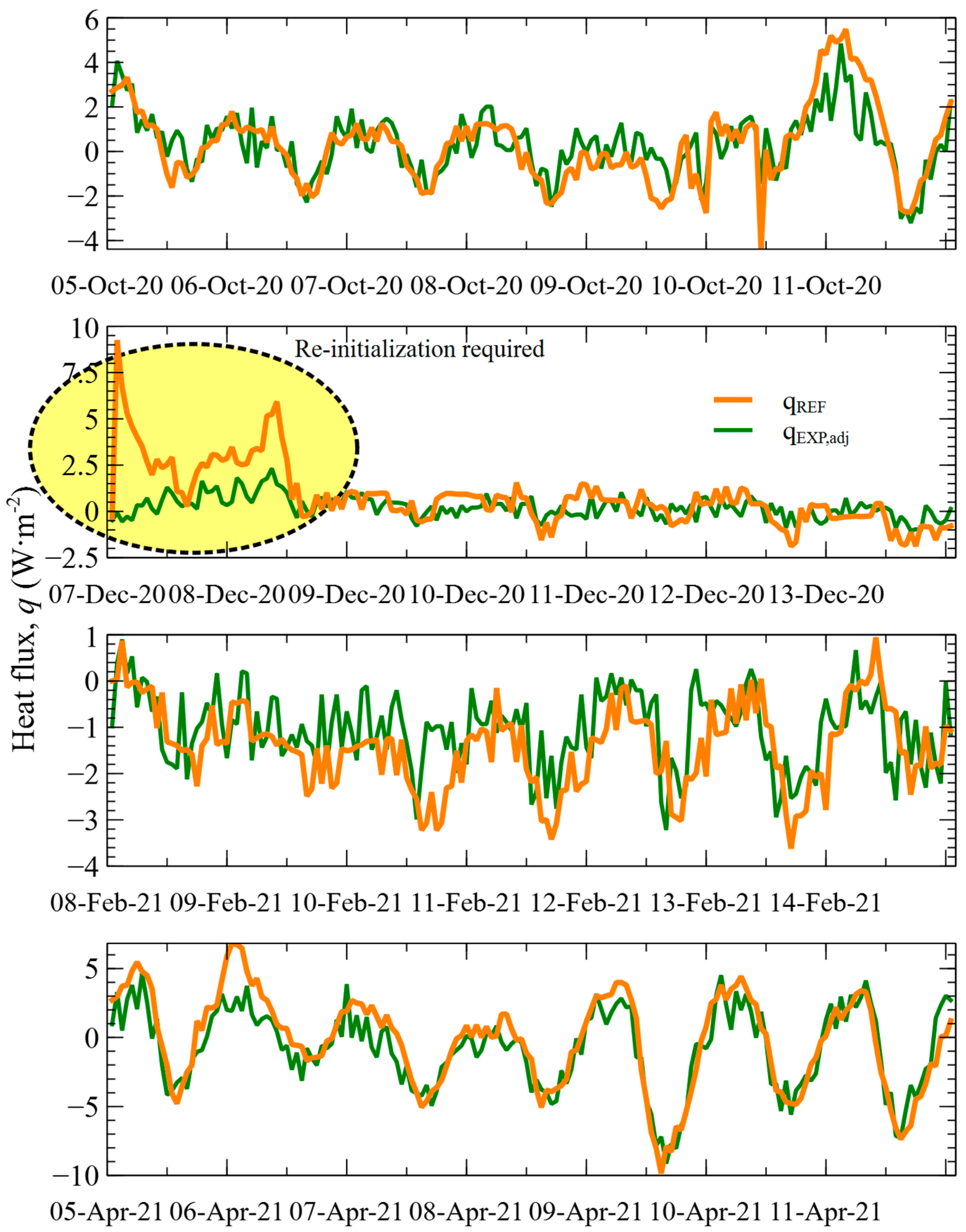
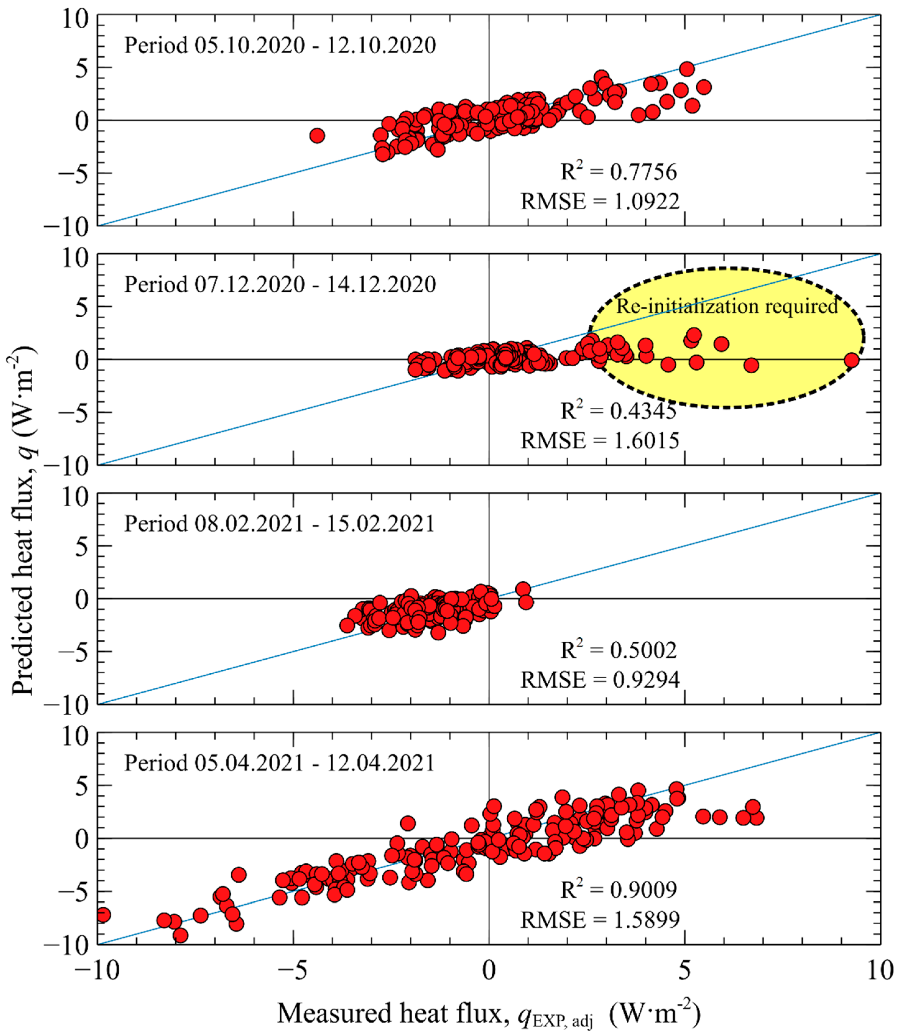
3.3. Phase 3—Sensor Performance Verification

With the adjusted sensitivity of the heat flux sensor, the sensor sensitivity adjustment procedure could proceed to the verification stage using data from Phase 3. For the verification, four testing periods between autumn 2020 and spring 2021 that followed the adjustment periods were selected (see Table 1 and Figure 6) and performance data was obtained for those periods. The idea of the verification was to prove the stability of the performed adjustment on blind data in the periods sufficiently close to the point of readjustment. The performance data included indoor and surface temperature measurements as well as outdoor climatic data for the simulation of the thermal response of the wall. Similarly to the previous steps, the surface heat fluxes q_IN and q_OUT were derived from experimental-computational data and compared against the output of the adjusted heat flux sensor.

Generally, the most important data reflecting the accuracy of demonstrated application are shown in Figure 11. Here, various accuracies of the adjusted sensor can be observed within the periods of verification. To provide a better insight into the accuracy of the adjusted heat flux sensor, a regression analysis of data was done and the R-squared values together with RMSE were determined for each period. The results of regression analysis are shown in Figure 12. The discrepancy from the adjustment phase as discussed in Section 3.2 (see Figure 9) has been clearly projected into this verification (as marked in Figure 11). Since the verification was done on the periods that followed the adjustment periods immediately, some performance deviations in the period 7 December 2020–13 December 2020 were anticipated. This observation underlines the need for a proper re-initialization based on detailed surveillance and analysis of the adjusted performance to optimize the computational model and to adapt the proposed procedure to changing environmental conditions.

It should be noted that the investigated object serves recreational purposes which is typical of a seasonal regime of occupation. As for this, some parts of the object, such as the entry foyer or some technical rooms, are considered “free-running” rooms, i.e., without space heating and/or cooling during the entire year. This stands also for the room, where all the sensors were placed, which is apparent from the interior temperature development during the measuring period (see Figure 6). This fact can seriously affect the results as the operating conditions might dramatically change over time, which can affect the sensor performance and physical behavior of construction materials.

3.4. Validation of the Self-Adjustment Technique

For the validation, the field data were obtained between 1 March 2022 and 15 March 2022. In reference to the beginning of the experiment, the validation period corresponded to the interval between Days 568 and 582. Right after the validation period, the self-adjustment of the HFP01SC sensor sensitivity was done to update the accuracy and validate the outputs from the HFP01 sensors. The self-adjustment of the sensitivity was done several times, while the interval between individual executions was at least 6 h as recommended by the manufacturer. The summary of experimental data obtained during the validation period is shown in Figure 13. The thermoelectric voltage in this figure refers to the output recorded on the HFP01SC and will be further processed with the adjusted sensitivity determined through the adjusting procedure. The data from the sensor sensitivity self-adjustment procedure are summarized in

Table 4. Results of self-adjustment procedure of HFP01SC sensor sensitivity.

	USC (mV)	Ucurrent (mV)	Rcurrent (Ω)	Rheater (Ω)	Aheater (m2)	SSC (V·m2·W−1)
1	3.012	0.596	10	99.2 ± 1.0	(3885 ± 136) × 10−6	(60.34 ± 2.41) × 10−6
2	2.958	0.594	10	99.2 ± 1.0	(3885 ± 136) × 10−6	(65.69 ± 2.63) × 10−6
3	2.925	0.592	10	99.2 ± 1.0	(3885 ± 136) × 10−6	(65.42 ± 2.62) × 10−6
4	2.938	0.593	10	99.2 ± 1.0	(3885 ± 136) × 10−6	(65.46 ± 2.62) × 10−6
5	2.859	0.588	10	99.2 ± 1.0	(3885 ± 136) × 10−6	(64.66 ± 2.59) × 10−6
SSC = (64.31 ± 2.57) × 10−6 V·m2·W−1

.

After performing the sensitivity adjustment, the thermoelectric voltage from Figure 13 was divided by the new sensitivity to obtain the time-resolved heat flux which served as the reference value in the validation procedure. Simultaneously, the heat fluxes q_IN(t) and q_OUT(t), obtained from Steps 2–4 as described in Section 2.2, were plotted in Figure 14. Prior to the calculation of q_IN(t) and q_OUT(t), the computational model was adjusted according to Step 1 of the proposed procedure to achieve the best performance of the semi-virtual environment. The heat transfer coefficient α was optimized to 5.0 W·m⁻²·K⁻¹ producing the least difference (RMSE = 0.2627) between computationally and experimentally determined surface temperatures T_s,sim(t) and T_s,exp(t), respectively. The validation data presented in Figure 14 represent the key input for the validation of the presented technique itself. Here, the reference heat flux from the high-sensitive probe HFP01SC was compared with the computational-experimental one (q_REF), which substitutes the electrically generated flux in the proposed sensor adjustment technique. The correspondence of the heat flux data in Figure 14 is very good, which can be considered a good result of the validation procedure showing that the heat flux from the semi-virtual environment was obtained with reasonable accuracy, and could be used as a target value in any subsequent calibration or sensitivity adjustment.

4. Discussion

The results presented in the previous subsections demonstrated that heat flux measurements in buildings need to reflect specific requirements given by the experimental conditions. Besides the changing environment, which might be typical for “free-running” buildings, the selection of appropriate heat flux probes is crucial for obtaining accurate data. However, the results reported in this paper showed that even such issues can be effectively addressed if a proper approach is chosen.

The analysis of the experimental data underlined the necessity of sensor re-calibration as the heat flow rate between the indoor environment and building walls may dramatically change during the measurement as a consequence of changing environmental conditions. The adaptive sensitivity adjustment proved that the heat transfer coefficient α was changed during the measurement which could be attributed to different conditions during model initialization [38,39]. Therefore, careful monitoring of environmental conditions as well as field variables should be done to provide sufficient data for a decision on whether re-initializations and/or re-adjustments are required and what is the recommended time span for performing the individual procedural steps.

A periodic calibration is often required in the building sector to ensure reliable quality of measured quantities. The conventional approach of calibration, on the other hand, may be exceptionally difficult to perform as the sensors might be difficult to reach or can’t be removed from the construction due to ongoing measurement. There have been limited studies published in the literature focusing on addressing those issues [40,41,42]. The novel approaches are mostly called virtual experiments, online calibrations, self-calibrations, or various combinations using these or similar other terms. However, most of the research published in the literature tends to prefer the traditional ways of sensor calibrations, which depend primarily on the type of used sensors [43,44,45]. The importance of heat flux monitoring and analysis in the field of building and civil engineering can be documented by reference to numerous works that have been published recently [46,47,48,49,50,51,52,53,54,55]. Also, the variety of those applications proves the importance of heat flux analysis that spans across multiple disciplines. Heat flux measurement is a key part of practically any thermal performance analysis [46,52,53,55], experimental validation of thermal properties of novel materials or building components [47,49,54], monitoring of thermal performances of buildings or their parts [48,50,51], etc. Therefore, the quality and accuracy of heat flux measurement should be always maintained at a high level, especially when long-term monitoring and observations are required [49,50,51]. In the field of heat flux monitoring, the producers brought new types of sensors with self-calibration capability, which clearly documents the awareness of the necessity for sensor recalibration during experimental measurement. The proposed method may contribute to the state-of-the art in this respect with the utilization of standard probes without advanced features, thus, providing high-tech solutions at standard costs. Also, the proposed approach can be applied “ex-post” to existing experimental data if some discrepancy is detected and appropriate environmental data are available along with heat flux variations. The accuracy of the proposed technique depends mostly on the selected re-adjustment period. Shorter periods bring higher accuracy to the heat flux measurement as the approach may efficiently reflect and address the changing environmental conditions. Basically, the readjustment can be triggered by user-defined values describing the change of environmental conditions or scheduled in regular periods. Consequently, a novel time-saving solution for maintenance-free application may be proposed as an alternative to traditional laboratory techniques.

5. Conclusions

In this paper, a smart adjustment technique for sensitivity enhancement of the surface heat flux probes was designed and validated in a critical experiment performed in real conditions. The proposed technique was based on combining the experimental and computational data to define a prescribed heat flux, thus omitting the need for traditional hardware equipment that would have to be used to perform the sensor performance check in the standard way. The proposed method allows the heat flux to be determined using raw data from the heat flux sensor without a need to interfere with the ongoing experiment. As such, the sensor sensitivity can be automatically adjusted during the measurement based on the surveillance of experimental variables. The applicability of the proposed method was demonstrated and validated in a real experiment. The following conclusions can be drawn, based on the performance analysis, to summarize the main outcomes of the research:

• Factory calibration of heat flux sensors is not always sufficient as the real experimental conditions may differ from those effective during the calibration. Also, some errors may arise from the type of installation of the heat flux sensors which can subsequently affect the sensitivity of the sensor.
• Continuous monitoring of heat flow sensor performance and silent checking of their accuracy allows the proposed technique to be applied instantaneously during the ongoing experiment without interfering with experimental apparatus or taking technological breaks required for sensor manipulation or replacement.
• The proposed approach is suitable for both short-term and long-term heat flux measurements while bringing an entirely new potential for maintenance-free applications. However, a qualified decision on sensor sensitivity re-adjustment or re-initialization of the computational model running in the background is crucial to ensure high accuracy of the method.
• The principles of the adaptive re-adjustments of heat flux sensor performance allow for their integration into automatic systems and smart HVAC technologies to efficiently control the indoor environment and thermal comfort of residential buildings based on real-time performance data.
• Although the validation was performed with sufficient accuracy, the additional testing would be beneficial to include various conditions, surface materials, or different kinds of probes. Such a complex validation should be considered an essential precondition.

References

1. Wang, S.; Chen, Y. Transient Heat Flow Calculation for Multilayer Constructions Using a Frequency-Domain Regression Method. Build. Environ. 2003, 38, 45–61. [Google Scholar] [CrossRef]
2. Zhang, Y.; Sun, X.; Medina, M.A. Calculation of Transient Phase Change Heat Transfer through Building Envelopes: An Improved Enthalpy Model and Error Analysis. Energy Build. 2020, 209, 109673. [Google Scholar] [CrossRef]
3. Fu, T.; Zong, A.; Zhang, Y.; Wang, H.S. A Method to Measure Heat Flux in Convection Using Gardon Gauge. Appl. Therm. Eng. 2016, 108, 1357–1361. [Google Scholar] [CrossRef]
4. Purpura, C.; Trifoni, E.; Petrella, O.; Marciano, L.; Musto, M.; Rotondo, G. Gardon Gauge Heat Flux Sensor Verification by New Working Facility. Measurement 2019, 134, 245–252. [Google Scholar] [CrossRef]
5. Gardon, R. An Instrument for the Direct Measurement of Intense Thermal Radiation. Rev. Sci. Instrum. 2004, 24, 366. [Google Scholar] [CrossRef]
6. Kidd, C.T.; Nelson, C.G. How the Schmidt-Boelter Gage Really Works. In Proceedings of the 41st International Instrumentation Symposium, Aurora, CO, USA, 7–11 May 1995. [Google Scholar]
7. Kidd, C.T.; Adams, J.C. Fast-Response Heat-Flux Sensor for Measurement Commonality in Hypersonic Wind Tunnels. J. Spacecr. Rockets 2012, 38, 719–729. [Google Scholar] [CrossRef]
8. Lam, C.S.; Weckman, E.J.; Lam, C.S.; Weckman, E.J. Steady-State Heat Flux Measurements in Radiative and Mixed Radiative–Convective Environments. Fire Mater. 2009, 33, 303–321. [Google Scholar] [CrossRef]
9. Mocikat, H.; Herwig, H. Heat Transfer Measurements with Surface Mounted Foil-Sensors in an Active Mode: A Comprehensive Review and a New Design. Sensors 2009, 9, 3011–3032. [Google Scholar] [CrossRef]
10. Lakatos, Á.; Kovács, Z. Comparison of Thermal Insulation Performance of Vacuum Insulation Panels with EPS Protection Layers Measured with Different Methods. Energy Build. 2021, 236, 110771. [Google Scholar] [CrossRef]
11. Ballestrín, J.; Estrada, C.A.; Rodríguez-Alonso, M.; Pérez-Rábago, C.; Langley, L.W.; Barnes, A. Heat Flux Sensors: Calorimeters or Radiometers? Solar Energy 2006, 80, 1314–1320. [Google Scholar] [CrossRef]
12. Sharkov, A.V.; Korablev, V.A.; Nekrasov, A.S.; Minkin, D.A.; Fadeeva, S.V. A Radiometer for Measuring High-Intensity Heat Flux Density and a Method of Calibrating It. Meas. Tech. 2012, 54, 1276–1279. [Google Scholar] [CrossRef]
13. Childs, P.R.N.; Greenwood, J.R.; Long, C.A. Heat Flux Measurement Techniques. Proc. Inst. Mech. Eng. C J. Mech. Eng. Sci. 1999, 213, 655–677. [Google Scholar] [CrossRef]
14. Nakos, J. Description of Heat Flux Measurement Methods Used in Hydrocarbon and Propellant Fuel Fires at Sandia; Sandia National Laboratories: Albuquerque, NM, USA; Livermore, CA, USA, 2010. [Google Scholar]
15. Levinson, R.; Chen, S.; Ferrari, C.; Berdahl, P.; Slack, J. Methods and Instrumentation to Measure the Effective Solar Reflectance of Fluorescent Cool Surfaces. Energy Build. 2017, 152, 752–765. [Google Scholar] [CrossRef]
16. ASTM C177-19; Standard Test Method for Steady-State Heat Flux Measurements and Thermal Transmission Properties by Means of the Guarded-Hot-Plate Apparatus. ASTM International: West Conshohocken, PA, USA, 2019.
17. ASTM C518-17; Standard Test Method for Steady-State Thermal Transmission Properties by Means of the Heat Flow Meter Apparatus. ASTM International: West Conshohocken, PA, USA, 2017.
18. Lakatos, Á.; Csík, A.; Csarnovics, I. Experimental Verification of Thermal Properties of the Aerogel Blanket. Case Stud. Therm. Eng. 2021, 25, 100966. [Google Scholar] [CrossRef]
19. ASTM C1130-21; Standard Practice for Calibration of Thin Heat Flux Transducers. ASTM International: West Conshohocken, PA, USA, 2021.
20. ASTM C1363-19; Standard Test Method for Thermal Performance of Building Materials and Envelope Assemblies by Means of a Hot Box Apparatus. ASTM International: West Conshohocken, PA, USA, 2019.
21. ASTM C1114-06; Standard Test Method for Steady-State Thermal Transmission Properties by Means of the Thin-Heater Apparatus. ASTM International: West Conshohocken, PA, USA, 2019.
22. ISO 8302:1991; Thermal Insulation—Determination of Steady-State Thermal Resistance and Related Properties—Guarded Hot Plate Apparatus. Technical Committee: ISO/TC 163; International Organization for Standardization: Geneve, Switzerland, 1991.
23. ASTM C1046-95R21; Standard Practice for In-Situ Measurement of Heat Flux and Temperature on Building Envelope Components. ASTM International: West Conshohocken, PA, USA, 2021.
24. ASTM C1155-95R21; Standard Practice for Determining Thermal Resistance of Building Envelope Components from the In-Situ Data. ASTM International: West Conshohocken, PA, USA, 2021.
25. Zarr, R.R.; Martinez-Fuentes, V.; Filliben, J.J.; Dougherty, B.P. Calibration of Thin Heat Flux Sensors for Building Applications Using ASTM C 1130. J. Test. Eval. 2001, 29, 293–300. [Google Scholar] [CrossRef]
26. HFP01SC Brochure HFP01SC Self-Calibrating Heat Flux Sensor Brochure. Available online: www.hukseflux.com (accessed on 17 April 2022).
27. FHF04SC Brochure FHF04SC Self-Calibrating Heat Flux Sensor with Integrated Heater Brochure. Available online: www.hukseflux.com (accessed on 17 April 2022).
28. Info; huksefluxcom FHF05 Series Heat Flux Sensors User Manual. Available online: www.hukseflux.com (accessed on 18 July 2024).
29. Maděra, J.; Kočí, V.; Kočí, J.; Černý, R. Physical and Mathematical Models of Hygrothermal Processes in Historical Building Envelopes. AIP Conf. Proc. 2017, 1906, 140003. [Google Scholar] [CrossRef]
30. Maděra, J.; Kočí, J.; Kočí, V.; Kruis, J. Parallel Modeling of Hygrothermal Performance of External Wall Made of Highly Perforated Bricks. Adv. Eng. Softw. 2017, 113, 47–53. [Google Scholar] [CrossRef]
31. Kočí, V.; Jerman, M.; Pavlík, Z.; Maděra, J.; Žák, J.; Černý, R. Interior Thermal Insulation Systems Based on Wood Fiberboards: Experimental Analysis and Computational Assessment of Hygrothermal and Energy Performance in the Central European Climate. Energy Build. 2020, 222, 110093. [Google Scholar] [CrossRef]
32. Künzel, H.M. Simultaneous Heat and Moisture Transport in Building Components: One-and Two-Dimensional Calculation Using Simple Parameters; Fraunhofer IRB Verlag Suttgart; IRB-Verlag: Stuttgart, Germany, 1995. [Google Scholar]
33. Jerman, M.; Keppert, M.; Výborný, J.; Černý, R. Hygric, Thermal and Durability Properties of Autoclaved Aerated Concrete. Constr. Build. Mater. 2013, 41, 352–359. [Google Scholar] [CrossRef]
34. Kočí, V.; Maděra, J.; Jerman, M.; Žumár, J.; Koňáková, D.; Čáchová, M.; Vejmelková, E.; Reiterman, P.; Černý, R. Application of Waste Ceramic Dust as a Ready-to-Use Replacement of Cement in Lime-Cement Plasters: An Environmental-Friendly and Energy-Efficient Solution. Clean. Technol. Environ. Policy 2016, 18, 1725–1733. [Google Scholar] [CrossRef]
35. User Manual FHF01, Hukseflux Thermal Sensors. Available online: https://www.hukseflux.com/uploads/product-documents/FHF01_manual_v2006.pdf (accessed on 14 December 2021).
36. User Manual HFP01 & HFP03, Heat Flux Plate/Heat Flux Sensor, Hukseflux Thermal Sensors. Available online: https://www.hukseflux.com/uploads/product-documents/HFP01_HFP03_manual_v1721.pdf (accessed on 14 December 2021).
37. Info; huksefluxcom Self-Calibrating Heat Flux Sensor TM Hukseflux Thermal Sensors. HFP01SC User Manual Self-Calibrating Heat Flux Sensor TM Hukseflux Thermal Sensors. Available online: www.hukseflux.com (accessed on 5 April 2022).
38. Maffulli, R.; He, L. Wall Temperature Effects on Heat Transfer Coefficient for High-Pressure Turbines. J. Propuls. Power 2014, 30, 1080–1090. [Google Scholar] [CrossRef]
39. Janssen, H. Dependence of Heat Transfer Coefficients on the Wall Temperature Shape and Consequences for the Calculation of Overall Heat Transfer Coefficients for Heat Exchangers. Heat Transf. Coeff. 1996, 31, 153–161. [Google Scholar] [CrossRef]
40. Yu, Y.; Li, H. Virtual In-Situ Calibration Method in Building Systems. Autom. Constr. 2015, 59, 59–67. [Google Scholar] [CrossRef]
41. Bychkovskiy, V.; Megerian, S.; Estrin, D.; Potkonjak, M. A Collaborative Approach to In-Place Sensor Calibration. Lect. Notes Comput. Sci. 2003, 2634, 301–316. [Google Scholar] [CrossRef]
42. Dulev, V.; Ermishin, S.; Khoteev, N.; Lopatin, A.; Shabanov, P.; Menshikov, A.; Startsev, A. Automated Measuring System Designed to Calibrate Measuring Devices Using Virtual Standards® Technology. In Proceedings of the AUTOTESTCON, San Antonio, TX, USA, 20–23 September 2004; pp. 158–164. [Google Scholar] [CrossRef]
43. Sapozhnikov, S.Z.; Mityakov, V.Y.; Mityakov, A.V.; Pokhodun, A.I.; Sokolov, N.A.; Matveev, M.S. The Calibration of Gradient Heat Flux Sensors. Meas. Tech. 2012, 54, 1155–1159. [Google Scholar] [CrossRef]
44. Sharkov, A.V.; Korablev, V.A.; Makarov, D.S.; Minkin, D.A.; Nekrasov, A.S.; Gordeichik, A.A. Measurement of High-Density Heat Flux Using an Automated Installation. Meas. Tech. 2016, 59, 67–69. [Google Scholar] [CrossRef]
45. Zhang, J.; Mei, G.; Bao, T.; Yan, L.E. An Experimental Study on Thermal Analyses of Crushed-Rock Layers with Single-Size Aggregates. Cold Reg. Sci. Technol. 2019, 160, 110–118. [Google Scholar] [CrossRef]
46. Ha, T.-T.; Feuillet, V.; Waeytens, J.; Zibouche, K.; Peiffer, L.; Garcia, Y.; le Sant, V.; Bouchie, R.; Koenen, A.; Monchau, J.-P.; et al. Measurement Prototype for Fast Estimation of Building Wall Thermal Resistance under Controlled and Natural Environmental Conditions. Energy Build. 2022, 268, 112166. [Google Scholar] [CrossRef]
47. Chihab, Y.; Bouferra, R.; Garoum, M.; Essaleh, M.; Laaroussi, N. Thermal Inertia and Energy Efficiency Enhancements of Hollow Clay Bricks Integrated with Phase Change Materials. J. Build. Eng. 2022, 53, 104569. [Google Scholar] [CrossRef]
48. Al-Absi, Z.A.; Hafizal, M.I.M.; Ismail, M. Experimental Study on the Thermal Performance of PCM-Based Panels Developed for Exterior Finishes of Building Walls. J. Build. Eng. 2022, 52, 104379. [Google Scholar] [CrossRef]
49. Balocco, C.; Pierucci, G.; de Lucia, M. An Experimental Method for Building Energy Need Evaluation at Real Operative Conditions. A Case Study Validation. Energy Build. 2022, 266, 112114. [Google Scholar] [CrossRef]
50. Briga-Sá, A.; Leitão, D.; Boaventura-Cunha, J.; Martins, F.F. Trombe Wall Thermal Performance: Data Mining Techniques for Indoor Temperatures and Heat Flux Forecasting. Energy Build. 2021, 252, 111407. [Google Scholar] [CrossRef]
51. Stella, P.; Personne, E. Effects of Conventional, Extensive and Semi-Intensive Green Roofs on Building Conductive Heat Fluxes and Surface Temperatures in Winter in Paris. Build. Environ. 2021, 205, 108202. [Google Scholar] [CrossRef]
52. Rincón-Casado, A.; Jara, E.Á.R.; Pardo, A.R.; Lissén, J.M.S.; Flor, F.J.S. de la Reducing the Cooling Energy Demand by Optimizing the Airflow Distribution in a Ventilated Roof: Numerical Study for an Existing Residential Building and Applicability Map. Appl. Sci. 2024, 14, 6596. [Google Scholar] [CrossRef]
53. Santos, P.; Abrantes, D.; Lopes, P.; Moga, L. The Relevance of Surface Resistances on the Conductive Thermal Resistance of Lightweight Steel-Framed Walls: A Numerical Simulation Study. Appl. Sci. 2024, 14, 3748. [Google Scholar] [CrossRef]
54. Küheylan, C.D.; Özkan, D.B. Experimental and Theoretical Study of Heat Transfer in a Chilled Ceiling System. Appl. Sci. 2024, 14, 5908. [Google Scholar] [CrossRef]
55. Harangozó, J.; Tureková, I.; Marková, I.; Hašková, A.; Králik, R. Study of the Influence of Heat Flow on the Time to Ignition of Spruce and Beech Wood. Appl. Sci. 2024, 14, 4237. [Google Scholar] [CrossRef]
Figure 1. Scheme of heat transfer in the surface element of building wall.
Applsci 14 07323 g001
Figure 2. Scheme of the adjustment approach with an independent validation.
Applsci 14 07323 g002
Figure 3. Experimental measurement and input data overview.
Applsci 14 07323 g003
Figure 4. The realization of the in-situ experiment.
Applsci 14 07323 g004
Figure 5. Extension of the experimental setup for the validation of the proposed technique.
Applsci 14 07323 g005
Figure 6. Experimental data for the demonstration of sensor calibration technique.
Applsci 14 07323 g006
Figure 7. Adjustment of the computational model.
Applsci 14 07323 g007
Figure 8. Adjusted performance of the computational model and its comparison with experimental data.
Applsci 14 07323 g008
Figure 9. Comparison of surface heat fluxes before calibration (Phase 2).
Applsci 14 07323 g009
Figure 10. Sensor performance after sensitivity adjustment (Phase 2).
Applsci 14 07323 g010
Figure 11. Performance verification of the self-adjustment technique.
Applsci 14 07323 g011
Figure 12. Regression analysis of the verification results.
Applsci 14 07323 g012
Figure 13. Experimental data for the validation of sensor sensitivity adjustment technique.
Applsci 14 07323 g013
Figure 14. Validation of the proposed sensitivity adjustment technique.
Applsci 14 07323 g014