Yolo Based Defects Detection Algorithm for EL in PV Modules with Focal and Efficient IoU Loss

Abstract

Considering the defect detection issues in electroluminescence (EL) of photovoltaic (PV) cell systems, lots of factors result in performance degradation, including defect diversity, data imbalance, scale difference, etc. Focal-EIoU loss, an effective defect detection solution for EL, is proposed based on the improved YOLOv5. Firstly, by analyzing the detection background and scale characteristics of EL defects, a binary classification is carried out in the system. Subsequently, a cascade detection network based on YOLOv5 is designed to further extract features from the binary-classified defects. The defect localization and classification are achieved in this way. To address the problem of imbalanced defect samples, a loss function is designed based on EIoU and Focal-F1 Loss. Experimental results are illustrated to show the effectiveness. Compared with the existing CNN-based deep learning approaches, the proposed focal loss calculation-based method can effectively improve the performance of handling sample imbalance. Moreover, in the detection of 12 types of defects, the Yolov5 algorithms can always obtain higher MAP (mean average precision) even with different parameter levels (Yolov5m: 0.791 vs. 0.857, Yolov5l: 0.798 vs. 0.862, Yolov5x: 0.802 vs. 0.867, Yolov5s: 0.793 vs. 0.865).

1. Introduction

Considering the energy efficiency improvement and carbon emission reduction, the demand for photovoltaic (PV) products is increasing. Meanwhile, it requires the PV inspection equipment to have the capabilities in mass-scale detection and possessing to realize the quality assessment of PV modules. In the quality inspection of PV modules, apart from the basic visual quality assessment, increasing attention has been raised to electroluminescence (EL) defect detection during practical industry applications. The detection principles are listed as follows: When a positive voltage is applied to the PV module, non-equilibrium charge carriers in the semiconductor material redistribute and recombine, emitting photons. These emitted photons are captured by EL detection equipment and converted into visible light signals. The optical sensors, such as CCD cameras, then capture these light signals. Through signal processing, the light signals are converted into a voltage format, generating an image that represents the surface current density distribution of the PV module [1]. By analyzing these images, the internal current transport and charge distribution within the PV module can be better understood, enabling assessment of the overall quality and performance.

However, the conventional manual inspection methods currently used in the PV inspection industry have become bottlenecks, restricting both the production efficiency and product quality of PV products due to their reliance on subjective judgment by inspection personnel. Manual inspection in PV product manufacturing leads to lower overall production efficiency and yield rates for component manufacturers, and the need for many inspectors further increases the labor cost of production. Although some EL image acquisition systems are equipped with automatic defect detection algorithms, their detection accuracy is not high enough to meet industrial production requirements. Therefore, these systems remain auxiliary tools in the production process and cannot achieve full automation. Furthermore, traditional defect detection algorithms [2,3,4,5] can achieve good detection results for a single type of defect, but they lack effectiveness in handling various defects with diverse morphologies and sizes on actual production lines, thereby facing limitations in terms of generalizability.

EL defect detection in PV modules is a typical multi-scale object detection problem [6]. Compared with natural image object detection problems, because of the large difference in defect scale and the imbalance of defect samples, this has always been a difficulty in the industry. Yang [7] used grayscale differences to extract texture attributes of defect regions for defect recognition, while Ko [8] introduced a strategy for detecting defects in multicrystalline silicon solar cells based on local segmentation and binary thresholding. However, these early strategies require manual feature selection, limiting their generality and accuracy. As scholars’ interest in this field has grown, new approaches have emerged, such as using Kalman filtering to track defect trajectories [9], wavelet image fusion with region sharpness enhancement [10], image matching and fusion techniques [11], and the adoption of Random Sample Consensus (RANSAC) algorithm to eliminate erroneous feature matching [12]. Nevertheless, these traditional methods are still limited by strict requirements for image stability and can only operate in specific environments, failing to fully adapt to the pace of modern efficient and intelligent manufacturing.

In 2017, a one-stage deep learning model [13] was used for defect detection in PV cell EL images, improving the challenges of complex background textures and imbalanced defect samples. The model achieved an accuracy of 74.7% for detecting two types of defects. In 2018, Bartler et al. [14] first validated the feasibility of using a Convolutional Neural Network (CNN) for EL image defect detection. In 2019, Liu built a deep convolutional neural network based on GoogLeNet [15] to detect four types of defects with an accuracy exceeding 85% and improved stability [16]. Subsequently, the VGG19 [17] model was also employed to predict the probability of defects in EL images. Additionally, VGG16 [18], ResNet50 [19], and BAF-CNN [20] have been used for defect detection and classification in EL images. Despite the continuous improvement in classification accuracy, challenges still exist, including limited recognition of defect types, lack of defect localization, large model parameters, and slow detection speed.

In 2018, Dong Mei [21] constructed a deep neural network using support vector machine sequences to achieve high-precision detection of color defects in continuous casting slabs [22]. From 2018 to 2020, many researchers developed Faster R-CNN [23,24] networks for detecting transmission line defects [25,26] and surface defects in industrial components [27,28,29,30], including defects in PV modules [28]. In 2019, Xu [31] and Tian et al. [32] improved the accuracy of PV module defect detection by building a solid-state drive architecture. In 2020, researchers began constructing retina networks [33] to detect small objects and subtle defects, aiming to strike a balance between speed and accuracy. Therefore, from a technical perspective, deep learning can be widely applied in product quality inspection.

From 2015 to 2023, the YOLO (You Only Look Once) series of algorithms underwent significant advancements, introducing YOLO [34], YOLOv2 [35], YOLOv3 [36], YOLOv4 [37], and the latest YOLOv5 models. These iterations propelled the field of target detection to unprecedented heights.

YOLOv5 stands out as the fifth-generation one-stage object detection algorithm, renowned for its compact model size and exceptional performance. It strikes a delicate balance between detection accuracy and speed across various real-world applications. Recent reports [38] indicate that YOLOv5 achieves mask detection in populations with an impressive accuracy exceeding 97%. Within the realm of photovoltaics, YOLOv5 has found utility in segmenting visible light images and pinpointing faults in infrared images [39]. Moreover, in fabric defect detection applications, the integration of attention mechanism modules has proven instrumental in enhancing the detection precision of YOLOv5 [40].

To address the constraints observed in existing research works, including shortcomings in defect type recognition, defect localization, large model parameters, and sluggish detection speeds, this study integrates the YOLOv5 algorithm with a cascaded detection model. The cascaded detection network is structured with both upstream and downstream components. A better-designed loss function can better extract defect characteristics. Combining the strengths of EIoU loss and Focal-F1 loss [26], an enhanced Focal-EIoU loss function is proposed and incorporated within the detection network, facilitating adaptive adjustments in the attention balance among various defect types during training, guided by sample distribution. The test outcomes showcase the superior detection capabilities of this novel approach, affirming its efficacy in overcoming the limitations highlighted in prior research.

2. Materials and Methods

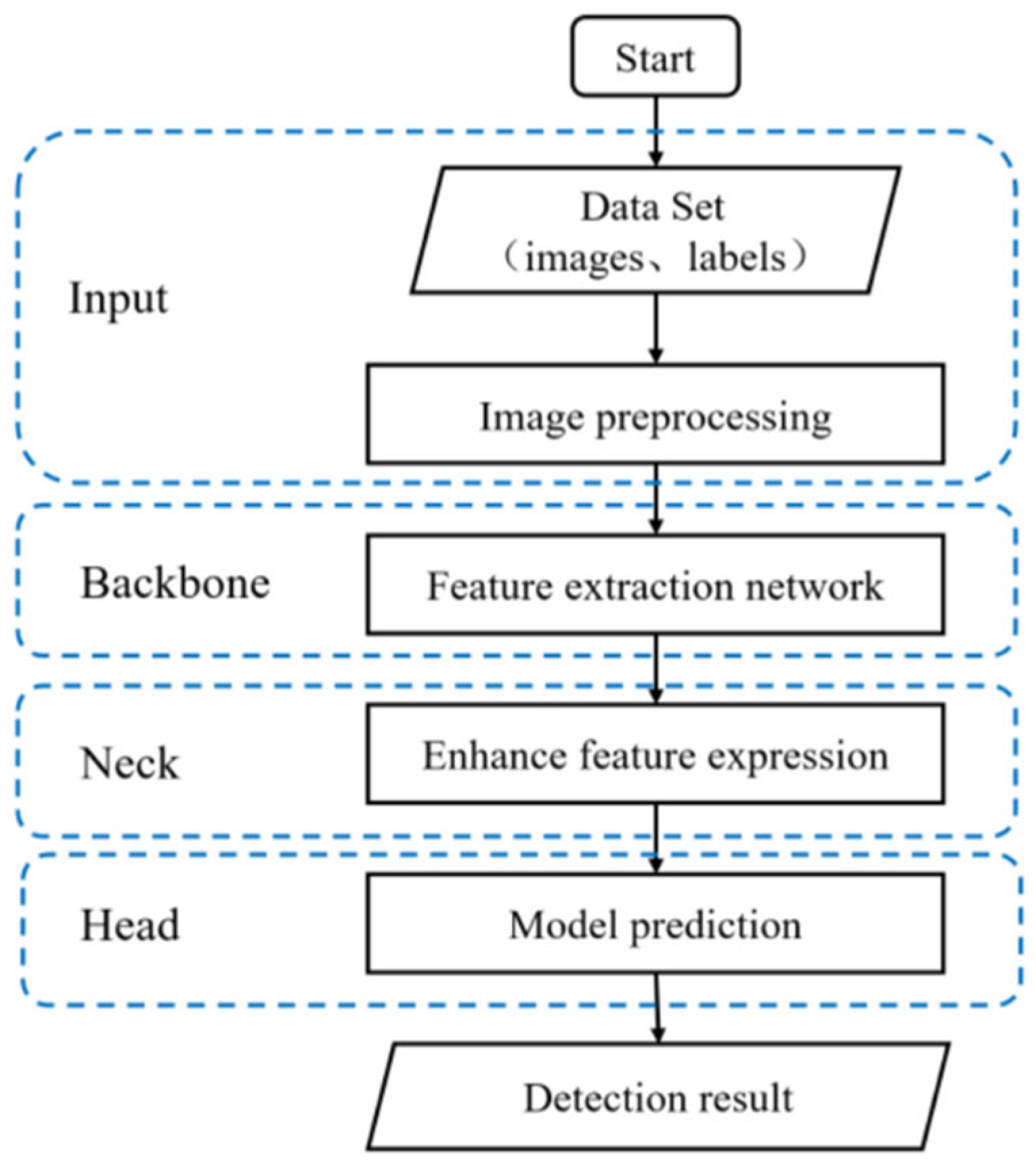
2.1. YOLOv5

The network structure of YOLOv5 mainly consists of four parts: Input, Backbone [41], Neck [42], and Head, as shown in Figure 1.

Incorporating Mosaic data augmentation at the input stage, YOLOv5 combines four randomly scaled, cropped, aligned, concatenated, and padded sample images to form a new composite sample image. This technique merges multiple images into a singular entity, thereby enhancing the image dataset and accelerating the training speed of the network. Moreover, this augmentation method not only diminishes the requirement for numerous GPUs but also implements adaptive anchor box computation to derive high-quality anchors. Additionally, it utilizes adaptive scaling to standardize the image sizes to an optimal dimension, further optimizing the training process.

The Backbone part adopts the New CSP-Darknet53 [40] model and utilizes the Focus module (Figure 2) to perform slicing operations, transforming the 640 × 640 × 3 image into a 320 × 320 × 12 tensor. The structure of CSP1_X is shown in Figure 3, where X represents the number of residual modules (Res units) in the structure. The CBL module consists of a convolutional layer, a batch normalization layer (BN), and an activation function (Hard-Swish activation function [43]). Each Res unit consists of a series of convolutional layers and a residual connection. The two convolutional layers (Conv) are used to adjust the number of channels in order to add the two calculations together (Concat).

In the Neck component, YOLOv5 integrates Feature Pyramid Network (FPN) and Path Aggregation Network (PAN) modules to bolster multi-scale feature representation and accurate localization details. The addition of CSP2_X intensifies the feature fusion from the preceding stage, as depicted in Figure 4. Within the Prediction segment, the GIoU_Loss function is utilized to determine the localization loss. This function aids in optimizing the model’s ability to precisely pinpoint objects within an image, enhancing the overall accuracy of the detection process.

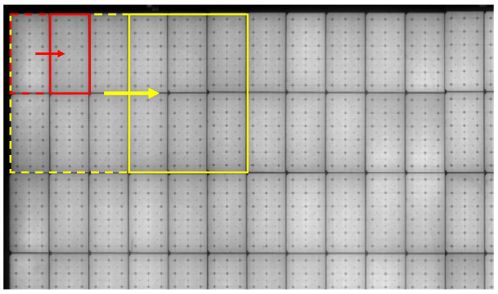
2.2. EL Images

The image data pertaining to PV modules examined in this study are sourced from Jiangsu Rituo Photovoltaic Company. The PV module products manufactured by the company are constructed by organizing PV cells in a 6-row by 21-column cell matrix configuration. Subsequently, these modules are subjected to EL detection for image capturing. Consequently, each EL image of a PV module comprises 126 cells, with each image size measuring 5328 × 3134 pixels.

The dataset encompasses 12 prevalent types of PV module EL defects. These defects are categorized into two main groups based on their size. The first category comprises large-sized defects (L-type), where the PV module serves as the backdrop, and the PV cells are identified as the targets. This group includes instances of current non-uniformity and dark areas. The second category encompasses small-sized defects (S-type), where the PV cells act as the background and specific regions within the cells are marked as the targets. This group includes various anomalies such as dark spots, black spots, broken grids, SE offset, false marks, branch occlusions, linear occlusions, fragments, flurry filaments, and cleaning traces. The characteristics and classifications of the complete set of 12 defects are visually depicted in Figure 5 and detailed in Table 3.

The utilization of deep learning algorithms for extracting defect features from PV module EL images presents notable challenges. Primarily, these images encompass a vast area and include substantial redundant information, rendering the detection of small-sized targets like dark spots and broken grids arduous using deep learning techniques. Moreover, there exists a substantial disparity in size among various defect types. For instance, the area contrast between broken grids and black cells exceeds a hundredfold. Furthermore, the distribution of samples across each defect class is uneven. To standardize the input for processing, images are typically rescaled and resized to a fixed dimension, often 640 × 640 pixels. However, in practical scenarios, the dimensions of PV module EL images (5325 × 3134 pixels) are considerably large, and this rescaling procedure can result in a notable loss of features, particularly for defects like dark spots and broken grids. This loss of detail can impede the accurate identification and characterization of such defects using deep learning methodologies.

Hence, a novel image segmentation strategy is introduced, employing a sliding window technique to accomplish the region segmentation of PV module EL images. This approach enables the extraction and learning of small-sized defect features from the segmented samples. By segmenting the images into smaller, more manageable sections, the system can focus on analyzing and understanding the intricate details of defects like dark spots and broken grids, enhancing the overall accuracy and effectiveness of the defect detection process. The minimum input size of the models is 640 × 640 pixels. In order not to lose information during image preprocessing, we want the sample size to be smaller than the input size of the model. Therefore, samples with the size of 248 × 504 pixels (single cell) were used to allow the model to learn the details of the defects. In order to learn the background features, we also take six adjacent cells as a sample, which contains the edge features of the battery; therefore, the model will not misjudge the edge of the battery as a defect.

The segmentation process involves utilizing two different sizes of sliding windows: 248 × 504 pixels and 756 × 1010 pixels, as illustrated in Figure 6, to partition the images into segments. Following this segmentation, image segments devoid of defects are discarded, resulting in augmented image samples. Within these augmented samples, small-sized target defects are annotated, while the annotations for large-sized defects, such as dark areas and current non-uniformity, are preserved from the original samples. This methodology ensures that the system focuses on learning and detecting the intricate features of the small-sized defects while retaining information about the larger defects for comprehensive analysis and detection.

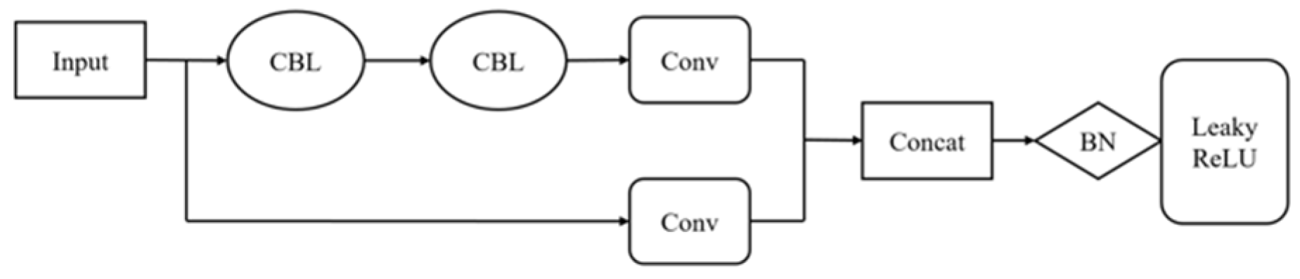
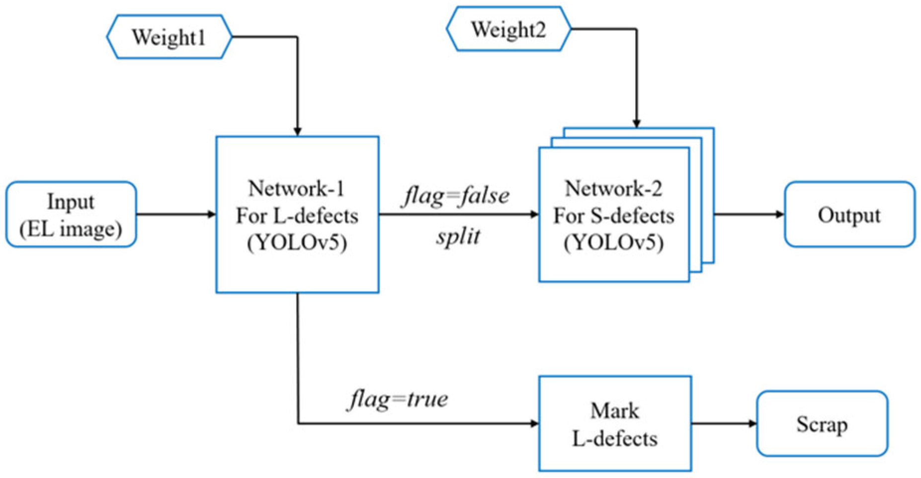
2.3. Cascaded Detection Network

In the realm of industrial production processes, catering to real-time detection demands requires defect detection algorithms to balance both detection speed and accuracy effectively. YOLOv5 stands out as an end-to-end one-stage model that eliminates the necessity of generating candidate regions. Instead, it conducts simultaneous regression for object localization and classification tasks. With its compact model size and rapid detection capabilities, YOLOv5 emerges as a fitting choice for EL defect detection in PV modules.

To enhance the detection proficiency for small-sized targets, a detection model comprising two cascaded YOLOv5 detection modules is proposed. These two modules are specifically tailored to identify two categories of defects: L-type defects and S-type defects. By harnessing the synergy between upstream and downstream processes, precise detection of all defect types is achieved, as demonstrated in Figure 7. This cascaded approach ensures comprehensive defect detection by segmenting the task into specialized modules, each adept at handling specific defect types, thereby enhancing the overall accuracy and efficiency of the detection system.

During the detection process, the input EL images $x$ are processed through ${Network}_1$ to determine the presence of L-type defects, as specified in Equations (1) and (2), resulting in ${Output}_1$.

$${Input}_1=x$$

(1)

$${Output}_1={Network}_1\left(x\right)$$

(2)

Then, as shown in Equations (3)–(5), the EL images are segmented into 21 regions through image segmentation processing, and each region is then input into ${Network}_2$ for S-type defect detection, resulting in ${Output}_2$. Finally, the detection results from the cascaded networks are integrated, mapped back onto the PV module’s EL image, and outputted. The final network output results ${Output}_3$ is given in Equation (6).

$$x\stackrel{split}{\to }X=\left\{x_1,x_1,\dots ,x_{21}\right\}$$

(3)

$${Input}_2=X$$

(4)

$${Output}_2=\sum _{i=1}^{21}{Network}_2\left(x_i\right)$$

(5)

$${Output}_3={Output}_1{+Output}_2$$

(6)

In industrial engineering, streamlining the detection process can significantly enhance efficiency. Following the PV module’s EL quality standards, upon detecting an L-type defect (such as uneven current distribution and dark spots) in a PV module, the module is designated as a defective product and necessitates additional processing at the factory. During the detection process, the detection results from ${Network}_1$ can be saved in a $flag$ variable. If the $flag$ is True, the detection result is directly outputted. If the $flag$ is False, the input is passed to ${Network}_2$ The simplified network output ${Output}_4$ is given in Equation (7).

$${Output}_4=\left\{\begin{array}{c}{Output}_{1}flag=True\\ {Output}_{2}flag=False\end{array}\right.$$

(7)

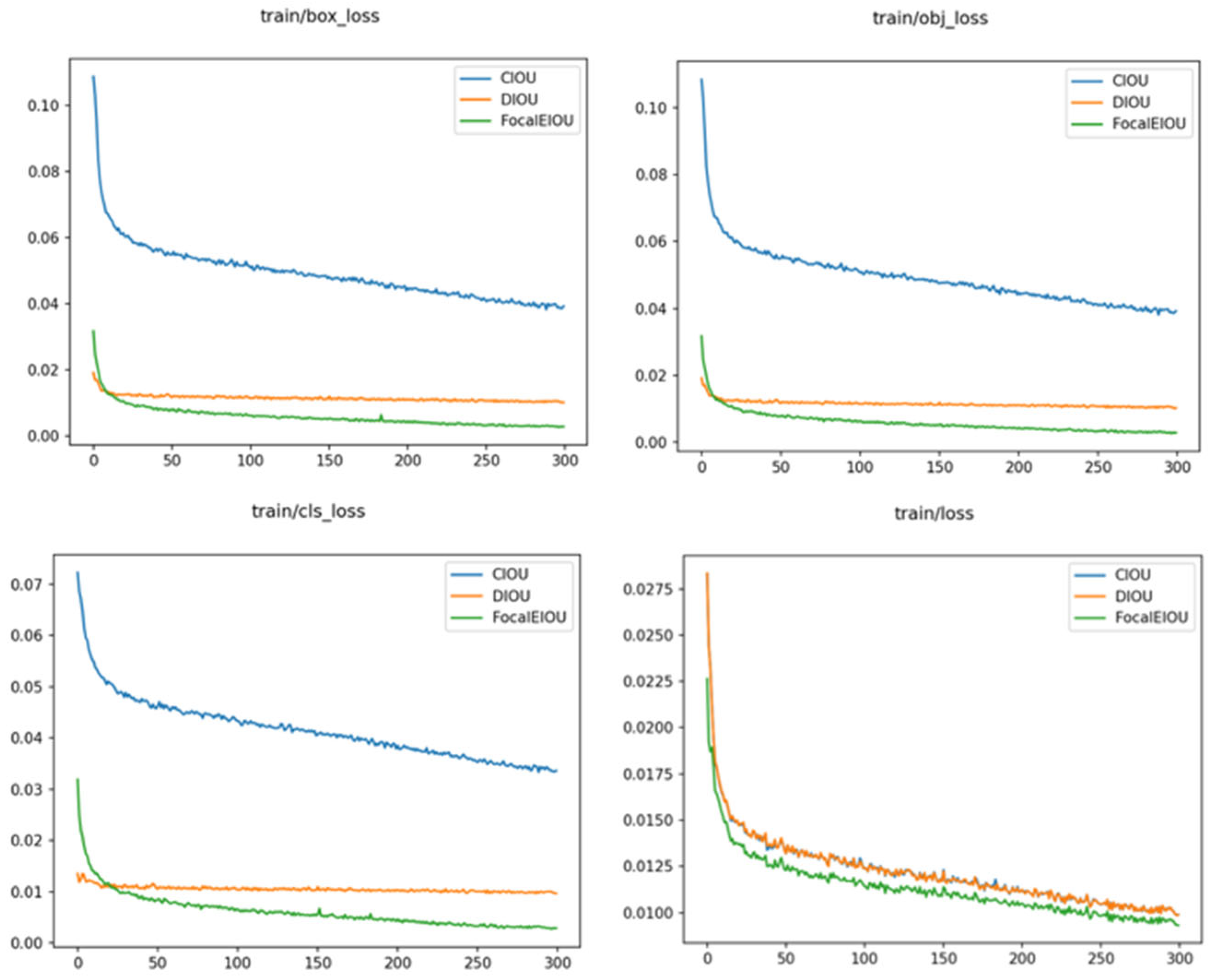
2.4. Focal-EIoU Loss

The EIoU loss function is designed to enhance the precision and effectiveness of bounding box regression in object detection tasks. This loss function optimizes target detection by focusing on three key aspects as follows:

• Center Point Distance Loss: This component aims to minimize the distance between the center points of the predicted bounding box and the ground truth bounding box. By doing so, it improves the accuracy of localizing the object within the bounding box;
• Consideration of Size Differences: EIoU penalizes discrepancies in width and height between the predicted bounding box and the ground truth bounding box. This penalty mechanism ensures that the predicted bounding box closely aligns with the shape and size of the actual object, thereby refining the detection accuracy;
• Incorporation of Minimum Enclosing Box Size: By integrating the size of the minimum enclosing box that encompasses both the predicted and ground truth bounding boxes into the loss function, EIoU becomes more attuned to the object’s size and position. This inclusion enhances the sensitivity of the loss function to variations in object size and spatial orientation, contributing to more precise object localization.

The EIoU loss function is expressed as shown in Equation (8).

$$\begin{gathered} {Loss}_{EIoU}=L_{IoU}+L_{dis}+L_{asp} \\ =1-IoU+{\displaystyle \frac{{\rho }^2\left(b,b^{gt}\right)}{c^2}}+{\displaystyle \frac{{\rho }^2\left(w,w^{gt}\right)}{c_w^2}}+{\displaystyle \frac{{\rho }^2\left(h,h^{gt}\right)}{c_h^2}} \end{gathered}$$

(8)

where $b,w,h$ represent the center coordinates, width, and height of the predicted box while $b^{gt},w^{gt},h^{gt}$ correspond to the center coordinates, width, and height of the annotated box. $\rho \left(b,b^{gt}\right)$ quantifies the Euclidean spatial distance between the centers of the two boxes, and $c,c_w,c_h$ represent the diagonal length, width, and height of the minimum enclosing box for the two boxes, respectively.

To address the issue of class imbalance in classification tasks, Focal Loss has been proposed as a specially designed loss function that effectively tackles this challenge. The Focal Loss function is expressed in Equation (9).

$${Loss}_{FocaL}=-{{\alpha }_t\left(1-p_t\right)}^{\gamma }\log \left(p_t\right)$$

(9)

where ${\alpha }_t$ is used to adjust the ratio of positive and negative samples, $\gamma$ is a parameter controlling the model’s focus on easy and hard-to-classify samples, and $p_t$ is the class probability.

In the training phase of neural networks, a large number of predicted bounding boxes have low IoU ratios with the ground truth boxes, indicating poor sample quality. Learning from these low-quality samples can result in significant loss oscillation, negatively affecting the model training process. To address the issue of class imbalance in regression tasks and enhance the contribution of high-quality samples during neural network learning, an improved version of Focal Loss called Focal-L1 Loss is proposed [26]. The gradient of Focal-L1 Loss is expressed as in Equation (10).

$$g\left(x\right)=\left\{\begin{array}{c}-x\alpha \ln \left(\beta x\right),0<x\le 1,{\displaystyle \frac{1}{e}}\le \beta \le 1\\ -\alpha \ln \left(\beta \right),x>1,{\displaystyle \frac{1}{e}}\le \beta \le 1\end{array}\right.$$

(10)

where $\alpha$ is used to constrain the gradient intensity, and $\beta$ is used to control the curvature of the curve, ensuring that the gradient intensity falls within the range of (0,1). By taking the derivative of the gradient function, we obtain the loss function expression of Focal-L1 Loss, which can be denoted as in Equation (11).

$$L_f\left(x\right)=\left\{\begin{array}{c}-{\displaystyle \frac{\alpha x^2\left(2\ln \left(\beta x\right)-1\right)}{4}},0<x\le 1;{\displaystyle \frac{1}{e}}\le \beta \le 1\\ -\alpha \ln \left(\beta \right)x+C,x>1;{\displaystyle \frac{1}{e}}\le \beta \le 1\end{array}\right.$$

(11)

where $C$ is a constant to satisfy $C={\displaystyle \frac{2\alpha ln\beta +\alpha }{4}}$ in order to maintain the continuity of the loss function.

By accumulating the positional offsets between predicted bounding boxes and annotated ground truth boxes, the localization error of Focal-F1 Loss is computed. This localization error is given as follows.

$${Loss}_{local}={\sum }_{i\in \left\{x,y,w,h\right\}}{L}_f\left(\left|B_i-B_i^{gt}\right|\right)$$

(12)

By combining EIoU-Loss and Focal-F1 Loss, we obtain the expression for Focal-EIoU Loss as shown in Equation (13).

$${Loss}_{\mathrm{F}\mathrm{o}\mathrm{c}\mathrm{a}\mathrm{l}-\mathrm{E}\mathrm{I}\mathrm{o}\mathrm{U}}={IoU}^{\gamma }{Loss}_{EIoU}$$

(13)

In Equation (13), IoU and γ jointly determine the degree of outlier suppression in the loss function. When the parameter γ is escalated, the model demonstrates an intensified capability to suppress outlier samples; nonetheless, this elevation could potentially result in a deceleration of the convergence speed. Selecting the assessment of model performance as the benchmark through empirical investigations, it has been ascertained that establishing γ at a value of 0.5 strikes an optimal equilibrium between the suppression efficacy and the pace of convergence [44,45]. Consequently, γ is stipulated as 0.5 in this context as the designated standard.

3. Results

The experiments were conducted using the Windows 10 operating system and the PyTorch framework. The specific configuration is listed in

Table 1. Experimental environment and configuration.

Environment	Configuration
CPU	Intel(R) Core(TM) i7-10700 CPU @ 2.90 GHz 2.90 GHz
GPU	NVIDIA GeForce GTX 3060
System	Windows 10
Language	Python 3.8
Architecture	Pytorch

.

The dataset employed in this research comprises EL images of photovoltaic components obtained during real production operations. The initial data images exhibit a resolution of 5328 × 3134 pixels. Specifically, we isolated EL images featuring solely S-type defects and applied image segmentation techniques to generate samples sized at 248 × 504 pixels and 756 × 1010 pixels. These segmented EL images were then merged with the original EL images containing L-type defects and annotated utilizing LabelImg, an image annotation tool. As a result, a dataset comprising 2044 sample images is obtained and divided into a train set and test set by 4:1. As shown in Figure 8, the number of different samples is uneven.

In this study, ablation experiments were conducted based on YOLOv5 and three loss functions: DIoU, CIoU, and Focal-EIoU. We focused on learning the features of 12 types of EL defects in photovoltaic components.

The decrease of box_loss means that the model can accurately predict the location of the target; the decrease of obj_loss means that the model can correctly identify the target in the image; the decrease of cls_loss means that the model has higher accuracy in different categories. As shown in Figure 9, after adding focal_eiou_loss to the loss function, lower box_loss, box_loss, and cls_loss were obtained, thus obtaining lower loss in total, which proved that the proposed Focal-EIoU achieves significant performance advantages in terms of convergence speed and final convergence results.

Precision (P) and Recall (R) are important metrics for evaluating object detection algorithms, and their definitions are shown in Equations (14) and (15).

$$P={\displaystyle \frac{TP}{TP+FP}}$$

(14)

$$R={\displaystyle \frac{TP}{TP+FN}}$$

(15)

where TP represents the number of correctly detected objects, FP represents the number of false positives, and FN represents the number of false negatives.

F1 is a comprehensive metric that measures the precision and recall of a system. The relationship between F1 and P, as well as R, can be expressed as in Equation (16).

$$F1={\displaystyle \frac{P\times R}{P+R}}$$

(16)

The higher the P and R, the better the performance of the model. After completing the model training, the trained model is evaluated by detecting EL images to validate its effectiveness. This paper compares the detection performance of the model based on four metrics: P, R, F1 score, and mean average precision (mAP). The experimental results are presented in

Table 2. Comparison of detection performance under the three loss functions.

Loss	P	R	F1	mAP
DIoU	0.724	0.826	0.858	0.819
CIoU	0.758	0.844	0.857	0.847
Focal-EIoU	0.792	0.850	0.933	0.865

.

Comparing the four detection performance metrics of YOLOv5s under the three loss functions, the proposed Focal-EIoU loss function in this paper achieves the best detection capability for the model, with mAP of 0.865 for the detection of 12 EL defects.

This paper uses mAP as the primary metric to evaluate the detection performance of the model and compares the detection capabilities of the three models for the 12 defects. The experimental results are shown in

Table 3. mAP for the 12 EL defects under three loss functions.

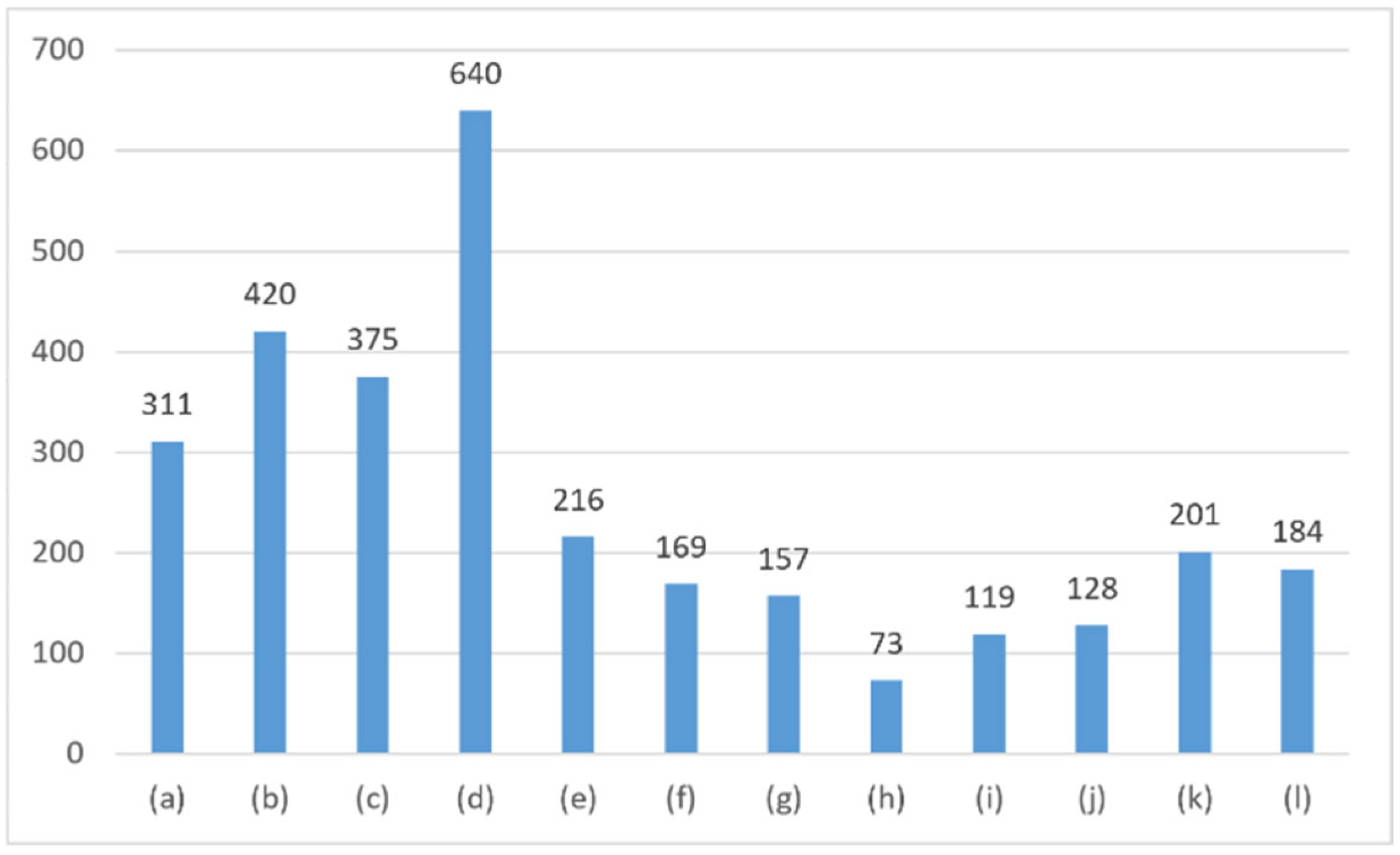
Defects	DIoU	CIoU	Focal-EIoU
(a) SE offset	0.714	0.721	0.837
(b) Dark spots	0.728	0.758	0.850
(c) Black spots	0.745	0.824	0.830
(d) Broken girds	0.822	0.765	0.866
(e) False marks	0.798	0.847	0.843
(f) Linear recessive cracks	0.743	0.775	0.827
(g) Branch recessive cracks	0.703	0.752	0.858
(h) Fragment	0.850	0.853	0.876
(i) Flurry filaments	0.761	0.810	0.855
(j) Cleaning traces	0.755	0.768	0.823
(k) Current unevenness	0.812	0.841	0.906
(l) Black cell	0.884	0.905	0.958

.

From Table 3, it can be seen that the YOLOv5s model with the introduced Focal-EIoU loss function shows significant improvement in detecting defects with scarce samples, such as fragments, filaments, and black spots. This indicates that the proposed method effectively addresses the issue of decreased detection capability caused by sample imbalance.

To further validate the effectiveness of our proposed method, we use SVM [22], Faster R-CNN [24], SSD, YOLOv3 [36], YOLOv4 [37], YOLOv6s [46], and YOLOv7s [47]. As listed in

Table 4. Comparison of object detection algorithms.

Algorithms	mAP	Speed
SVM [22]	0.648	500 ms
Faster RCNN [24]	0.837	50 ms
SSD	0.750	90 ms
YOLOv3 [36]	0.671	70 ms
YOLOv4 [37]	0.734	30 ms
YOLOv5s [40]	0.793	20 ms
YOLOv6s [46]	0.782	60 ms
YOLOv7s [47]	0.811	80 ms
Proposed	0.865	20 ms

, researchers used to do EL defect detection via SVM, Faster RCNN, and SSD algorithm. In our previous research, Yolov5s without Focal-EIoU loss achieved better performance in terms of both accuracy and speed. The proposed method outperformed the three algorithms used before and achieved better performance than other original Yolo series methods. Furthermore, we conducted experiments to improve the loss function on four distinct versions of the YOLOv5 model: YOLOv5m, YOLOv5l, YOLOv5x, and YOLOv5s, as listed in

Table 5. Performance when incorporating the Focal-EIOU loss with different YOLOv5 models * indicates using the Focal-EIOU loss instead of their original losses.

Method	mAP	Speed
YOLOv5m	0.791	23.8 ms
YOLOv5m *	0.857	23.8 ms
YOLOv5l	0.798	32.6 ms
YOLOv5l *	0.862	32.6 ms
YOLOv5x	0.802	46.8 ms
YOLOv5x *	0.867	46.8 ms
YOLOv5s	0.793	20.0 ms
YOLOv5s *	0.865	20.0 ms

.

In the realm of object detection algorithms, YOLOv5 stands out for its exceptional suitability in detecting defects within PV components. It excels in delivering real-time processing capabilities while maintaining optimal average accuracy in defect recognition tasks. Although YOLOv6s and YOLOv7s marginally outperform YOLOv5s in accuracy metrics, their intricate algorithm architectures and substantial parameter sizes notably impede detection speed. Consequently, YOLOv6s and YOLOv7s are not well-aligned with the real-time demands of defect detection in PV components, in contrast to the efficiency and effectiveness demonstrated by YOLOv5 in this specific application domain.

Based on the data presented in Table 5, it is evident that the Focal-EIoU approach yields enhancements in mean Average Precision (mAP) across all iterations of YOLOv5. Notably, among these variations, YOLOv5s emerges as a particularly optimal choice, striking a superior balance between speed and mAP. This equilibrium ensures the efficient and accurate detection of defects in PV modules, underscoring YOLOv5s as a robust solution capable of meeting the real-time demands of PV module defect detection while maintaining high accuracy levels.

The enhanced version of the YOLOv5s algorithm model showcases a significant advancement in performance, boasting a notable 7.2% rise in mean Average Precision (mAP), specifically for complex defects found in PV components. This enhancement elevates the mAP from 79.3% to 86.5%, indicating a substantial improvement in the model’s ability to accurately detect and classify intricate defects within PV components.

This remarkable performance boost not only underscores the efficacy of the improved YOLOv5s algorithm model but also highlights its considerable potential for industrial applications in PV component defect detection. By achieving higher accuracy rates for complex defects, the enhanced model contributes significantly to enhancing the quality control processes in the photovoltaic industry, ultimately leading to more reliable and efficient defect detection systems.

4. Conclusions

The specific industrial problem is generally the problem of sample imbalance, and it is very different from the artificially filtered natural image dataset. In this paper, we demonstrate that when using CNN-based deep learning networks for defect detection, calculating Focal-EIoU loss in the loss function can reduce the impact of sample imbalance and is effective in real industrial scenarios. In the experiment, we selected the Yolo series algorithm to test. These algorithms are composed of convolution layers with similar structures and different parameter numbers. We conducted ablation experiments on Yolov5 models with different parameters. Adding Focal-EIoU loss to the loss function can obtain a higher mAP (Yolov5m: 0.791 vs. 0.857, Yolov5l: 0.798 vs. 0.862, Yolov5x: 0.802 vs. 0.867, Yolov5s: 0.793 vs. 0.865), which has little effect on the speed of forward inference. Interestingly, we also compared the Yolov5 model with Focal-EIoU loss with other models in the Yolo series and found that while obtaining a higher mAP, the advantages in a small number of parameters and fast forward derivation speed were performed. Therefore, we believe that in real industrial application scenarios, the effect of increasing the number of parameters in the model may not necessarily be more than the impact of reducing sample imbalance. We suggest that the Focal-EIoU loss method should be tried more frequently in industrial defect detection experiments that lack sufficient samples.

References

- Hu, X.; Tang, W.; Bi, J.; Chen, S.; Yan, W. CNN-based model for cell extraction from PV modules with EL images for PV defects detection. In Proceedings of the Chinese Control Conference, Shanghai, China, 26–28 July 2021; pp. 221–225. [Google Scholar]
- Dou, Z. Research of Online Defects Detection for Solar Panel Base on the EL Image. Master’s Thesis, Zhejiang Sci-Tech University, Hangzhou, China, 2013. [Google Scholar]
- Wang, Z. Research on Defect Detection System for Solar Cells. Master’s Thesis, Hebei University of Technology, Tianjin, China, 2014. [Google Scholar]
- Wang, X.; Li, J.; Yao, M.; He, W.; Qian, Y. Solar cells surface defects detection based on deep learning. Pattern Recognit. Artif. Intell. 2014, 27, 517–523. [Google Scholar]
- Yu, Y.; Yin, G.; Yin, Y.; Du, L. Defect recognition for radiographic image based on deep learning network. Chin. J. Sci. Instrum. 2014, 35, 2012–2019. [Google Scholar]
- Chen, T.; Ding, S.; Chen, H.; Chen, C. High accuracy detection strategy for EL defects in PV modules based on machine learning. In Proceedings of the Asia-Pacific Conference on Intelligent Robot Systems, Tianjin, China, 1–3 July 2022; pp. 128–134. [Google Scholar]
- Yang, J.; Guo, J. Image texture feature extraction method based on regional average binary gray level difference co-occurrence matrix. In Proceedings of the International Conference on Virtual Reality and Visualization, IEEE Computer Society, Beijing, China, 4–5 November 2011; pp. 239–242. [Google Scholar]
- Ko, J.; Rheem, J. Defect detection of polycrystalline solar wafers using local binary mean. Int. J. Adv. Manuf. Technol. 2016, 82, 1753–1764. [Google Scholar] [CrossRef]
- Zou, Y.; Du, D.; Chang, B.; Ji, L.; Pan, J. Automatic weld defect detection method based on Kalman filtering for real-time radiographic inspection of spiral pipe. Ndt E Int. 2015, 72, 1–9. [Google Scholar] [CrossRef]
- Niu, Q.; Ye, M.; Lu, Y. Defect detection of small hole inner surface based on multi-focus image fusion. J. Comput. Appl. 2016, 36, 2912–2915. [Google Scholar]
- Frome, A.; Singer, Y.; Sha, F.; Malik, J. Learning globally-consistent local distance functions for shape-based image retrieval and classification. In Proceedings of the IEEE 11th International Conference on Computer Vision, Rio de Janeiro, Brazil, 14–21 October 2007; pp. 1–8. [Google Scholar]
- Zhou, A.; Shao, W.; Guo, J. An image mosaic method for defect inspection of steel rotary parts. J. Nondestruct. Eval. 2016, 35, 60. [Google Scholar] [CrossRef]
- Han, J. Research on Classification and Detection of Solar Cells EL Defects under Class Imbalance Situation. Master’s Thesis, Hebei University of Technology, Tianjin, China, 2020. [Google Scholar]
- Bartler, A.; Mauch, L.; Yang, B.; Reuter, M.; Stoicescu, L. Automated detection of solar cell defects with deep learning. In Proceedings of the 2018 26th European Signal Processing Conference (EUSIPCO), Rome, Italy, 3–7 September 2018; IEEE Press: New York, NY, USA, 2018; pp. 2035–2039. [Google Scholar]
- Simonyan, K.; Zisserman, A. Very deep convolutional networks for large-scale image recognition. arXiv 2014, arXiv:1409.1556. [Google Scholar]
- Liu, B.; Huang, X.; Yang, Q. Research on detection technology of photovoltaic cells based on GoogLeNet and EL. Electron. Prod. Reliab. Environ. Test. 2019, 1, 150–155. [Google Scholar]
- Deitsch, S.; Christlein, V.; Berger, S.; Buerhop-Lutz, C.; Maier, A.; Gallwitz, F.; Riess, C. Automatic classification of defective photovoltaic module cells in electroluminescence images. Sol. Energy 2019, 185, 455–468. [Google Scholar] [CrossRef]
- Kaur, A.; Kukreja, V.; Kumar, M.; Choudhary, A.; Sharma, R. A Fine-tuned Deep Learning-based VGG16 Model for Cotton Leaf Disease Classification. In Proceedings of the 2024 5th International Conference for Emerging Technology (INCET), Belgaum, India, 24–26 May 2024; pp. 1–4. [Google Scholar]
- Tang, W.Q.; Yang, Q.; Xiong, K. Deep learning -based automatic defect identification of the photovoltaic module using electroluminescence images. Sol. Energy 2020, 201, 453–460. [Google Scholar] [CrossRef]
- Su, B.; Chen, H.; Zhou, Z. BAF-detector: An efficient CNN-based detector for photovoltaic cell defect detection. IEEE Trans. Ind. Electron. 2022, 69, 3161–3171. [Google Scholar] [CrossRef]
- Dong, M. Research on Yarn-dyed Fabric Defect Detection and Classification based on Convolutional Neural Network. Master’s Thesis, Xi’an Polytechnic University, Xi’an, China, 2018. [Google Scholar]
- Hu, J.; Wang, X.; Liu, H. Defect detection of continuous casting slabs based on deep learning. J. Shanghai Univ. (Nat. Sci. Ed.) 2019, 25, 445–452. [Google Scholar]
- Ren, S.; He, K.; Girshick, R.; Sun, J. Faster R-CNN: Towards teal-Time object detection with region proposal networks. IEEE Trans. Pattern Anal. Mach. Intell. 2017, 39, 1137–1149. [Google Scholar] [CrossRef] [PubMed]
- Yang, Q.; Ma, S.; Guo, D.; Wang, P.; Lin, M.; Hu, Y. A small object detection method for oil leakage defects in substations based on improved faster-RCNN. Sensors 2023, 23, 7390. [Google Scholar] [CrossRef] [PubMed]
- Gu, C.; Zhe, L.; Shi, J. Detection for pin defects of overhead lines by UAV patrol image based on improved Faster-RCNN. High Volt. Eng. 2020, 46, 3089–3096. [Google Scholar]
- Tang, Y.; Han, J.; Wei, W. Research on part recognition and detection of transmission line in deep learning. Electron. Meas. Technol. 2018, 60–65. [Google Scholar]
- Dai, X.; Chen, H.; Zhu, C. Surface defect detection and realization of mental workpiece based on improved Faster-RCNN. Surf. Technol. 2020, 362–371. [Google Scholar]
- Guo, M.; Xu, H. Hot spot defect detection based on infrared thermal image and faster-RCNN. Comput. Syst. Appl. 2019, 265–270. [Google Scholar]
- Zhu, C.; Yang, Y. Online detection algorithm of automobile wheel surface defects based on improved Faster-RCNN model. Surf. Technol. 2020, 358–365. [Google Scholar]
- Guo, T.; Yang, H.; Shi, L. Self-explosion defect identification of insulator based on faster RCNN. Insul. Surge Arresters 2019, 183–189. [Google Scholar]
- Xu, X. Solar Cell Defect Detection Based on Deep Learning. Master’s Thesis, North University of China, Taiyuan, China, 2019. [Google Scholar]
- Tian, X.; Cheng, Y.; Chan, G. Detect and recognize hidden cracks in silicon chips on deep learning SSD algorithm. Mach. Tool Hydraul. 2019, 36–41. [Google Scholar]
- Lin, T.; Goyal, P.; Girshick, R.; He, K.; Dollár, P. Focal loss for dense object detection. IEEE Trans. Pattern Anal. Mach. Intell. 2017, 42, 2999. [Google Scholar]
- Redmon, J.; Divvala, S.; Girshick, R.; Farhadi, A. You only look once: Unified, real-time object detection. In Proceedings of the IEEE International Conference on Computer Vision, Las Vegas, NV, USA, 27–30 June 2016; pp. 779–788. [Google Scholar]
- Redmon, J.; Farhadi, A. YOLO9000: Better, faster, stronger. In Proceedings of the IEEE Conference on Computer Vision and Pattern Recognition, Honolulu, HI, USA, 21–26 July 2017; pp. 7263–7271. [Google Scholar]
- Redmon, J.; Farhadi, A. YOLOv3: An incremental improvement. In Proceedings of the IEEE Conference on Computer Vision and Pattern Recognition, Salt Lake City, UT, USA, 18–23 June 2018; pp. 7263–7271. [Google Scholar]
- Bochkovskiy, A.; Wang, C.; Mark-Liao, H. YOLOv4: Optimal Speed and Accuracy of Object Detection. In Proceedings of the IEEE/CVF Conference on Computer Vision and Pattern Recognition, Seattle, WA, USA, 13–19 June 2020; pp. 1544–1552. [Google Scholar]
- Alahmadi, A.; Rezk, H. A robust single-sensor MPPT strategy for a shaded photovoltaic-battery system. Comput. Syst. Sci. Eng. 2021, 37, 63–71. [Google Scholar] [CrossRef]
- Hong, F.; Song, J.; Meng, H.; Wang, R.; Fang, F.; Zhang, G. A novel framework for intelligent detection for module defects of PV plant combining the visible and infra-red images. Sol. Energy 2022, 236, 406–416. [Google Scholar] [CrossRef]
- Jin, R.; Niu, Q. Automatic fabric defect detection based on an improved YOLOv5. Math. Probl. Eng. 2021, 2021, 7321394. [Google Scholar] [CrossRef]
- Zhu, X. Design of barcode recognition system based on YOLOV5. In Proceedings of the 2021 3rd International Conference on Computer Modeling, Changsha, China, 23–25 July 2021; pp. 346–349. [Google Scholar]
- Jin, S.; Sun, L. Application of enhanced feature fusion applied to YOLOv5 for ship detection. In Proceedings of the 33rd Chinese Control and Decision Conference, Kunming, China, 22–24 May 2021; pp. 8–11. [Google Scholar]
- Dubey, S.; Singh, S.; Chaudhuri, B. Activation functions in deep learning: A comprehensive survey and benchmark. Neurocomputing 2022, 503, 92–108. [Google Scholar] [CrossRef]
- Wang, S.; Qu, Z.; Gao, L. Multi-spatial pyramid feature and optimizing focal loss function for object detection. IEEE Trans. Intell. Veh. 2024, 9, 1054–1065. [Google Scholar] [CrossRef]
- Wang, Y.; Tian, Y.; Cheng, J. An improved YOLOv7 method for vehicle detection in traffic scenes. In Proceedings of the 2023 35th Chinese Control and Decision Conference (CCDC), Yichang, China, 20–22 May 2023; pp. 766–771. [Google Scholar]
- Li, C.; Li, L.; Jiang, H.; Weng, K.; Geng, Y.; Li, L.; Ke, Z.; Li, Q.; Cheng, M.; Nie, W.; et al. YOLOv6: A Single-Stage Object Detection Framework for Industrial Applications. arXiv 2022, arXiv:2209.02976. [Google Scholar]
- Wang, C.; Bochkovskiy, A.; Liao, H. YOLOv7: Trainable Bag-of-Freebies Sets New State-of-the-Art for Real-Time Object Detectors. In Proceedings of the 2023 IEEE/CVF Conference on Computer Vision and Pattern Recognition (CVPR), Vancouver, BC, Canada, 17–24 June 2023; pp. 7464–7475. [Google Scholar]