Article

Multi-Body Dynamics Modeling and Simulation of Maglev Satellites

1
Graduate School, Space Engineering University, Beijing 101416, China
2
Department of Aerospace Science and Technology, Space Engineering University, Beijing 101416, China
*
Author to whom correspondence should be addressed.
Appl. Sci. 2024, 14(17), 7588; https://doi.org/10.3390/app14177588
Submission received: 25 April 2024 / Revised: 3 August 2024 / Accepted: 17 August 2024 / Published: 28 August 2024

Abstract

:
The Lorentz force magnetic levitation gim2bal stabilized platform (LFMP), as a new generation of high-precision turntable for maglev satellites, can meet the requirements of future spacecraft for ultra-high attitude pointing accuracy and stability. To solve the problem of three-module multi-body attitude control under maneuvering conditions, the platform subsystem is first dynamically modeled based on the second type of Lagrangian equation, and the payload subsystem is dynamically modeled based on the Newton–Euler method. Secondly, a multi-loop control system is designed, consisting of high-precision and fast attitude pointing control for the payload, position tracking control for the platform subsystem, and tracking control for the maglev module. The final simulation results verified the feasibility and effectiveness of the payload-centered control method. An evaluation of the stability with a specific model has been performed, and the attitude accuracy of the payload is within 0.00002° and the attitude stability is within 0.00005°/s.

1. Introduction

In order to improve the ground imaging capability of spaceborne payloads, current space missions have proposed the ability requirements for ultra-precision pointing and ultra-stable control of spaceborne imaging payloads [1]. The traditional connection method between the satellite body and the imaging payload is through mechanical bearings. Compared with mechanical bearings, magnetic levitation bearings have a longer service life, do not wear, do not require lubrication, and possess controllable dynamic characteristics. They can reduce the influence of high-frequency vibration in the satellite body on the pointing control of the imaging payload and improve the pointing control accuracy of the imaging payload [2,3].
Compared with magnetic resistance magnetic bearings, Lorentz force magnetic bearings have no iron loss, good linearity, larger control bandwidth, and higher control accuracy, and are an ideal suspension method in microgravity environments [4]. The Canadian Space Agency has developed a series of MIM systems that utilize Lorentz force actuators to achieve active isolation control, which can isolate small vibrations in the range of 0.01 Hz to 100 Hz and have been successfully applied to the MIR Space Station [5]. In 2016, Basovich et al. from Israel designed a high-precision positioning table iterative learning output controller with travel range limitations for a 6-DOF maglev platform with uncertain loads, ensuring that all balance points are within the system’s motion range [6].
In 2017, Dyck et al. from Columbia University proposed a 6-DOF (Degrees of Freedom) magnetic levitation turntable for precision positioning. The turntable uses Lorentz force to provide driving force, which can provide sub-micron accuracy in precision micro-machining applications [7]. The precise vacuum-compatible dual servo maglev platform developed by the Seoul team in South Korea in 2022 can achieve an accuracy of 10 nm [8].
Ren et al. have developed a set of 6-DOF vibration isolation equipment with reference to the MIM gravity vibration isolation equipment. At present, a prototype has been made, and good results have been achieved in experiments [9]. Zhang Wei from the Shanghai Satellite Engineering Research Institute studied a collaborative control method for the isolation of payload modules and platform modules, using the DFP (Disturbance Free Payload) satellite platform as a reference. They achieved high pointing accuracy and stability in attitude control, and verified the performance of the platform through mathematical simulation [10]. The Beijing 3 satellite adopts a magnetic levitation precise isolation platform 10°/s to achieve three super performance, with a maximum in orbit attitude maneuver of and a stability of the entire satellite attitude angular velocity better than 2 × 10⁻⁵°/s [11].
For magnetic levitation systems, the performance of linear controllers can only be accepted at the equilibrium point, and selecting nonlinear controllers can provide global stability to the system [12]. Quaternions, as an effective mathematical tool for describing rotation, are widely used in attitude control of magnetic levitation systems.
Magnetic levitation satellites have shown significant advantages in active vibration isolation. The Lorentz force maglev gimbal stable platform (LFMP), as a new generation of satellite payload platform for rapid spatial information acquisition, precise pointing and positioning, and continuous control and disturbance reduction, requires ultra-stable, ultra-static, and ultra-agile technologies as its core features.

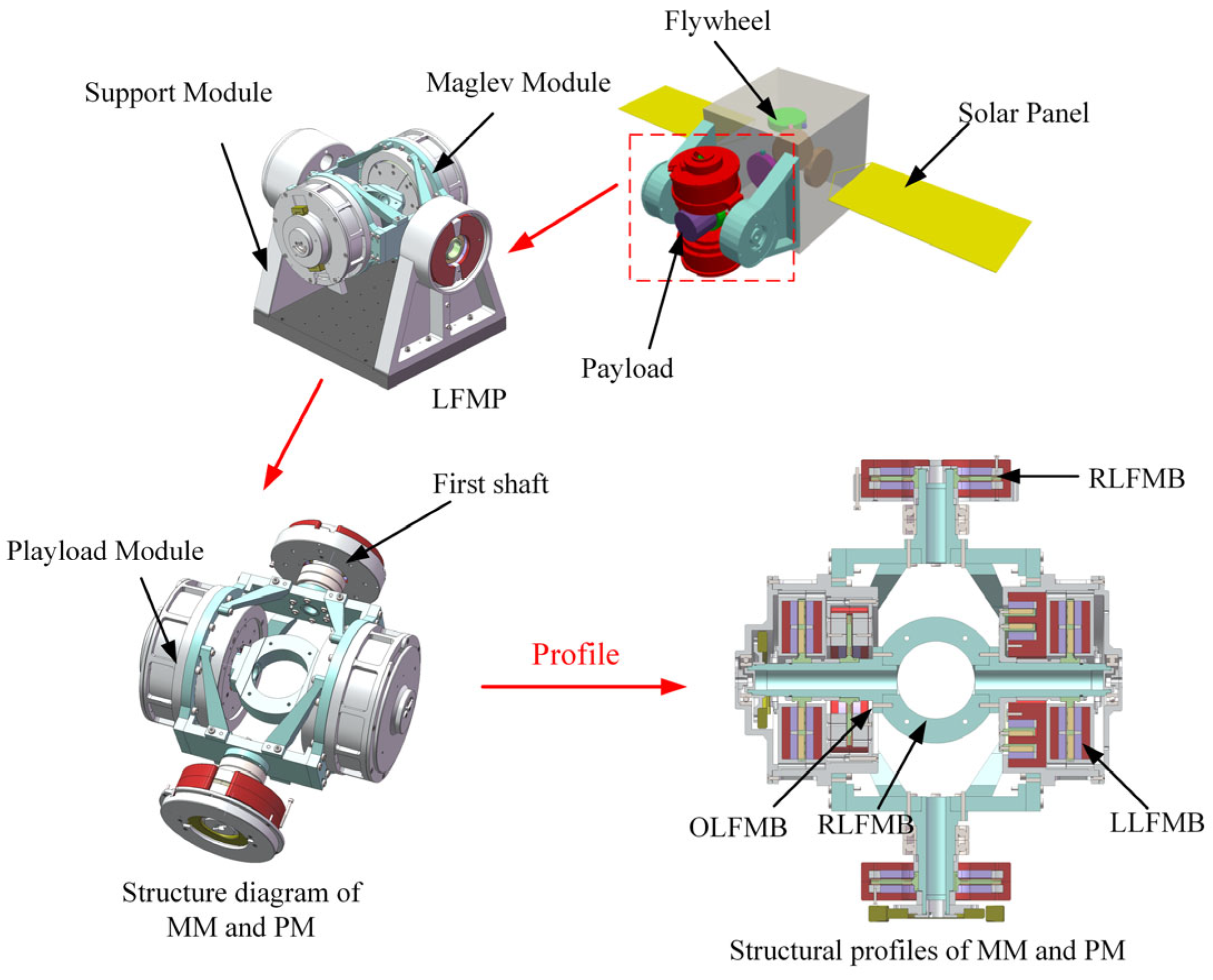
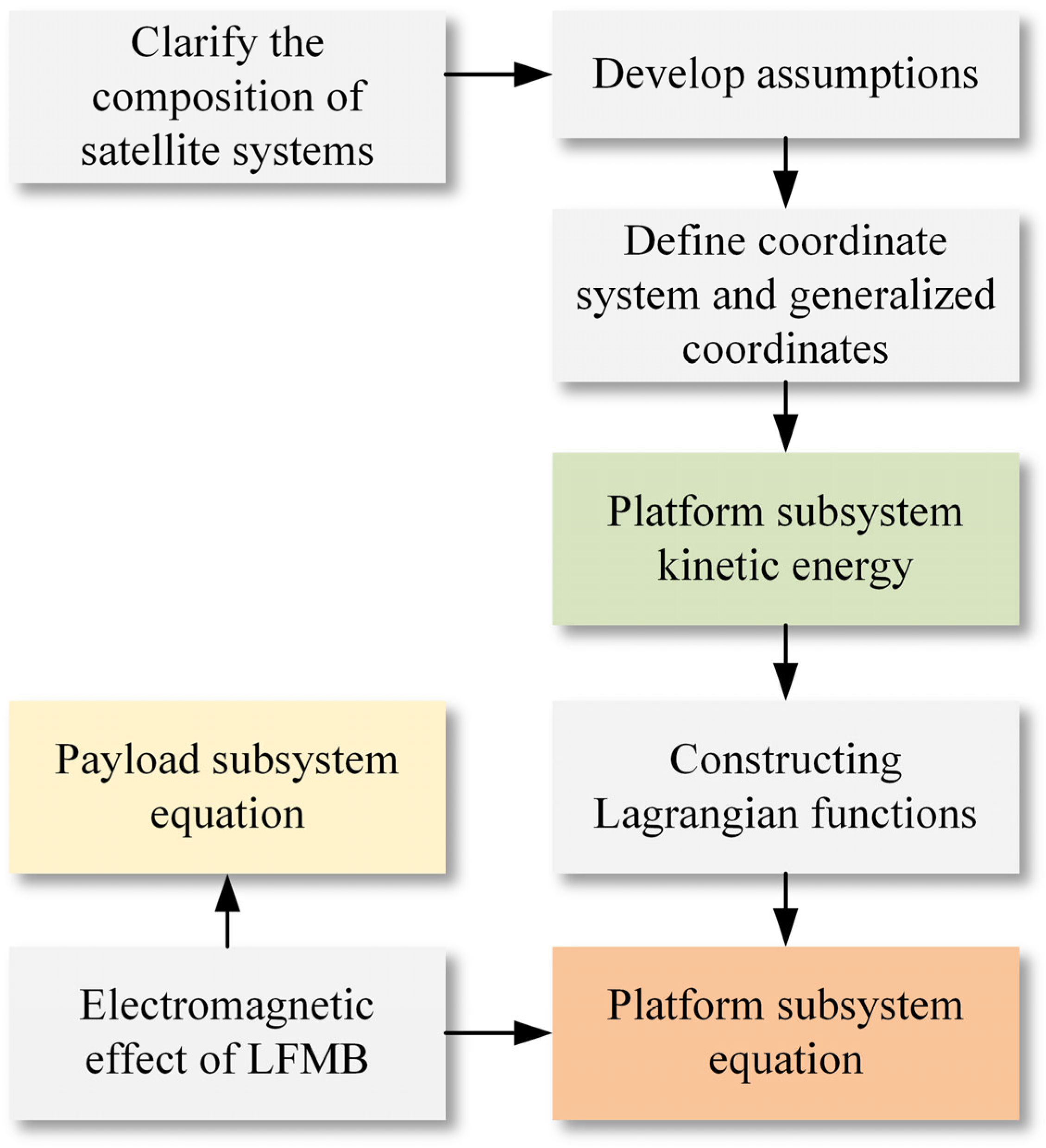
2. Modeling of Three Body Dynamics of Maglev Satellite

Unlike traditional satellite attitude control platforms, LFMP breaks the limitation that imaging satellites can only image after their attitude is stable. It combines the “instability” of attitude maneuver with the “stability” of high-precision imaging, allowing for continuous control of payload stability and pointing during ultra-agile maneuvers. LFMP inherits the non-contact advantages of the DFP platform and is divided into a multi-body structure with an SM (Support Module), MM (Maglev Module), and PM (Payload Module). At the same time, it uses Lorentz force magnetic bearings (LFMBs) support to stabilize and suspend the PM inside the MM. LFMP is jointly controlled by two poles, three rotating Lorentz force magnetic bearings (RLFMBs), coaxial two orthogonal Lorentz force magnetic bearings (OLFMBs), and a linear Lorentz force magnetic bearing (LLFMB) to complete the 7-DOF universal motion. The RLFMB controls the 2-DOF universal agile maneuver, the OLFMBs and LLFMBs control the 5-DOF stable suspension, and the three types of magnetic bearings work together to complete the complex 3-body 7-DOF motion. The structure of the maglev satellite is shown in Figure 1.
To improve the accuracy of dynamic modeling for satellite systems containing LFMBs, this paper establishes dynamic models for platform subsystems and payload subsystems based on the second type of Lagrange equation.
As shown in Figure 2, based on the constraint methods between the various components of the satellite system containing the LFMB, in the dynamic modeling process, it is considered that the SM and MM constitute the platform subsystem, while the PM and imaging payload constitute the payload subsystem. This section establishes dynamic models of the platform subsystem and payload subsystem based on the principle of the second type of Lagrange equation by formulating corresponding assumptions.
Assumption 1: 
Except for the bilateral solar wings of the satellite body, all components of the satellite system containing LFMP are assumed to be rigid bodies.
Assumption 2: 
When the PM is actively maneuvering, the rotational speed is low, and the changes in the moment of inertia during the rotation of the PM and MM are ignored.

2.1. Definition of Coordinate System and Position Vector

The coordinate systems used in the dynamic modeling process include the inertial coordinate system O i X i Y i Z i , orbital coordinate system O o X o Y o Z o , satellite platform system O b X b Y b Z b , MM system O r X r Y r Z r , and payload subsystem system O p X p Y p Z p . Figure 3 shows the definition and relative relationships of the platform subsystem centroid, payload subsystem centroid, satellite platform, and MM system.
The generalized coordinates for modeling are as follows: the projection X p f of the center of mass position of the platform subsystem in the inertial frame, the integral value ϑ b of the platform angular velocity vector projection in the platform system, the relative angle of the MM to the platform θ r , the projection X p l of the center of mass position of the payload subsystem in the inertial frame, and the integral value ϑ p of the angular velocity of the payload subsystem.
Referring to Figure 4, the vector definitions used in the dynamic modeling analysis of the platform subsystem are shown in Table 1.

2.2. Platform Subsystem Kinetic Energy

The absolute velocity v ¯ b of a certain quality element on the platform is:
v ¯ b = X ¯ ˙ p f + r ¯ ˙ b = X ¯ ˙ p f + r ¯ b + ω ¯ b × r ¯ b
where ω ¯ b is the platform angular velocity, and r ¯ b represents the relative derivative of r ¯ b relative to the platform system. By transferring Equation (1) to the platform system, it can be expressed as follows:
v b = A b T X ˙ p f + r ˙ b + r ˜ b T ω b
where v b is the projection of vector v ¯ b under the platform system, A b is the attitude transformation matrix of the platform system relative to the inertial frame, X p f is the projection of X ¯ p f under the inertial frame, r b = [ r b x , r b y , r b z ] T is the projection of r ¯ b under the platform system, ω b is the projection of ω ¯ b under the platform system, and r ˜ b represents the matrix operation as follows:
r ˜ b = 0 r b z r b y r b z 0 r b x r b y r b x 0
So the kinetic energy of the platform can be expressed as:
T b = 1 2 b v b T v b d m
Through simplification, it can be concluded that:
T b = 1 2 b X ˙ p f T X ˙ p f + 2 X ˙ p f T A b r ˙ b + 2 r ˙ b T r ˜ b T ω b + r ˙ b T r ˙ b + ω b T r ˜ b r ˜ b T ω + 2 X ˙ p f T A b r ˜ b T ω b b d m = 1 2 M b X ˙ p f T X ˙ p f + 1 2 ω b T J b c ω b + X ˙ p f T A b M b r ˙ b + 1 2 M b r ˙ b T r ˙ b + M b X ˙ p f T A b r ˜ b c T ω b + M b r ˙ b T r ˜ b c T ω b
where M b is the mass of the platform, J b c is the projection of the moment of inertia of the platform relative to its center of mass in this system, and r b c is the position vector from the center of mass of the platform subsystem to the center of mass of the platform.
The absolute velocity of a certain mass element on the MM is:
v ¯ r = X ¯ ˙ p f + r ¯ ˙ r + g ¯ ˙ r = X ¯ ˙ p f + r ¯ r + ω ¯ b × r ¯ r + ( ω ¯ b + ω ¯ r ) × g ¯ r = X ¯ ˙ p f + r ¯ r + ω ¯ b × ( r ¯ r + g ¯ r ) + ω ¯ r × g ¯ r
where ω ¯ r is the angular velocity of MM relative to the platform rotation. Represent the Equation (6) in the MM system as:
v r = C r T A b T X ˙ p f + C r T r ˙ r + ( C r T r ˜ r T + g ˜ r T C r T ) ω b + g ˜ r T ω r
where C r is the attitude transformation matrix of the MM system relative to the platform system, and v r , r r , g r , ω r are the projections of v ¯ r , r ¯ r , g ¯ r , ω ¯ r under the MM system, respectively. The kinetic energy of the MM can be expressed as:
T r = 1 2 r X ˙ p f T X ˙ p f + 2 X ˙ p f T A b C r ( C r T r ˜ r T + g ˜ r T C r T ) ω b + 2 X ˙ p f T A b C r g ˜ r T ω r + 2 ω b T ( r ˜ r C r + C r g ˜ r ) g ˜ r T ω r + ω r T g ˜ r g ˜ r T ω r + ω b T ( r ˜ r C r + C r g ˜ r ) ( C r T r ˜ r T + g ˜ r T C r T ) ω b + 2 r ˙ r T A b T X ˙ p f + r ˙ r T r ˙ r + 2 r ˙ r T C r g ˜ r T ω r + 2 r ˙ r T ( r ˜ r T + C r g ˜ r T C r T ) ω b d m
J r = r g ˜ r g ˜ r T d m is the projection of the moment of inertia of the MM relative to its origin in this system, and the relevant terms in the equation are expanded as follows:
ω b T r ( r ˜ r C r + C r g ˜ r ) ( C r T r ˜ r T + g ˜ r T C r T ) d m ω b = ω b T r ( r ˜ r r ˜ r T + r ˜ r C r g ˜ r T C r T + C r g ˜ r C r T r ˜ r T + C r g ˜ r g ˜ r T C r T ) d m ω b
The physical meaning of the integral sign on the right side of the equal sign in Equation (9) is the moment of inertia of the magnetic levitation module relative to the center of mass of the platform subsystem, denoted as J r c , which can be organized as:
J r c = M r r ˜ r r ˜ r T + M r r ˜ r C r g ˜ r c T C r T + M r C r g ˜ r c C r T r ˜ r T + C r J r C r T
where M r is the mass of the MM, g r c is the vector from the origin of the MM to the center of mass, denoted as ω r = D r θ ˙ r , D r = [ 1 , 0 , 0 ] T , and J r x are the O r X r -axis principal moments of inertia J r . Therefore, the kinetic energy of the MM body is further expressed as:
T r = 1 2 M r X ˙ p f T X ˙ p f + 1 2 ω b T J r c ω b + 1 2 J r x θ ˙ r 2 + M r X ˙ p f T A b r ˜ r T ω b + M r X ˙ p f T A b C r g ˜ r c T C r T ω b + M r X ˙ p f T A b C r g ˜ r c T D r θ ˙ r + M r ω b T r ˜ r C r g ˜ r c T D r θ ˙ r + ω b T C r J r D r θ ˙ r + M r r ˙ r T A b T X ˙ p f + M r r ˙ r T ( 1 2 r ˙ r + C r g ˜ r c T D r θ ˙ r + r ˜ r T ω b + C r g ˜ r c T C r T ω b )
Based on the above kinetic energy expression, the kinetic energy of the platform subsystem is:
T p f = T b + T r
Further considering the characteristics of the system center of mass, the following equation holds:
M b r b c + M r r r + C r g r c = 0
Therefore, in the kinetic energy expression of the platform subsystem, the following equation holds:
M b X ˙ p f T A b r ˜ b c T ω b + M r X ˙ p f T A b r ˜ r T ω b + M r X ˙ p f T A b C r g ˜ r c T C r T ω b = 0
M b r ˙ b c + M r r ˙ r + C r ω ˜ r g r c = 0
X ˙ p f T A b M b r ˙ b + M r X ˙ p f T A b C r g ˜ r c T D r θ ˙ r = 0
Considering that r ˙ b = r ˙ b c = r ˙ r holds, the following Equation (14) holds for the combination equation:
M b r ˙ b T r ˜ b c T ω b + M r r ˙ r T r ˜ r T ω b + M r r ˙ r T C r g ˜ r c T C r T ω b = r ˙ b T M b r ˜ b c T + M r C r g ˜ r c T C r T ω b = 0
In summary, Equation (12) can be simplified as:
T p f = 1 2 M p f X ˙ p f T X ˙ p f + 1 2 ω b T J p f ω b    + 1 2 J r x θ ˙ r 2 + ω b T ( M r r ˜ r C r g ˜ r c T + C r J r ) D r θ ˙ r    + 1 2 M r r ˙ r T C r g ˜ r c T D r θ ˙ r
According to Equation (15), it can be inferred that:
r ˙ b c = M r M C r g ˜ r c T D r θ ˙ r
Substituting Equation (19) into Equation (18) yields:
T p f = 1 2 M p f X ˙ p f T X ˙ p f + 1 2 ω b T J p f ω b    + 1 2 J r x θ ˙ r 2 1 2 M r 2 M D r T g ˜ r c g ˜ r c T D r θ ˙ r 2

2.3. Platform Subsystem Dynamics Equation

Substitute Equation (20) into the second Lagrangian equation:
d d T L p f q ˙ L p f q = Q
where L p f = T p f U p f is the Lagrangian function, where U p f = 0 , q is the generalized coordinate, and Q is the generalized force corresponding to the generalized coordinate.
The expansion of Equation (21) can be written as the following components to obtain the translational combined external force of the platform subsystem:
d d t L p f X ˙ p f L p f X p f = F p f
By substituting L p f into the above equation, we can obtain a translational equation for the platform:
M p f X ¨ p f = F p f
where F p f refers to the projection of F ¯ p f in the inertial frame. F ¯ p f including orbital control forces F ¯ k , space environment interference forces F ¯ d , and the reaction of electromagnetic forces F ¯ m applied by the MM to the PM, F p f can be expressed as:
F p f = F k + F d A b C r ( F u r + F a r + F l r )
where F k is the projection of F ¯ k in the inertial frame, F d is the projection of F ¯ d in the inertial frame, and F u r , F a r , F l r are the electromagnetic forces applied to the load compartment by the upper OLFMB, the LLFMB, and the lower OLFMB, respectively.
The expansion of Equation (21) can be written as the following components to obtain the driving torque of the MM:
d d t L p f θ ˙ r L p f θ r = τ r
By substituting L p f into the above equation, we can obtain the driving equation for the MM:
J r x M r 2 M D r T g ˜ r c g ˜ r c T D r θ ¨ r + ω ˙ b T R r D r + ω b T R ˙ r D r = τ r
where τ r is the moment of force exerted on the MM.

2.4. Payload Subsystem Dynamics Equation

Since the PM and payload can be viewed as a whole, the payload subsystem can establish dynamics based on the Newton–Euler equation of a single rigid body as follows:
M p l X ¨ p l = A b C r F u r + F a r + F l r
J p l ω ˙ p + ω ˜ p J p l ω p = r ˜ s u C p r F u r + r ˜ s a C p r F a r + r ˜ s l C p r F l r + C p r τ q
where M p l refers to the mass of the payload subsystem; X p l is the vector from the origin of the inertial frame to the center of mass; J p l is the moment of inertia; ω p is the payload angular velocity; r s u , r s a and r s l are the vectors of the electromagnetic force application points of the center of mass pointing upwards and downwards OLFMBs and LLFMBs, respectively; and C p r is the attitude transformation matrix of the relative payload subsystem of the MM.

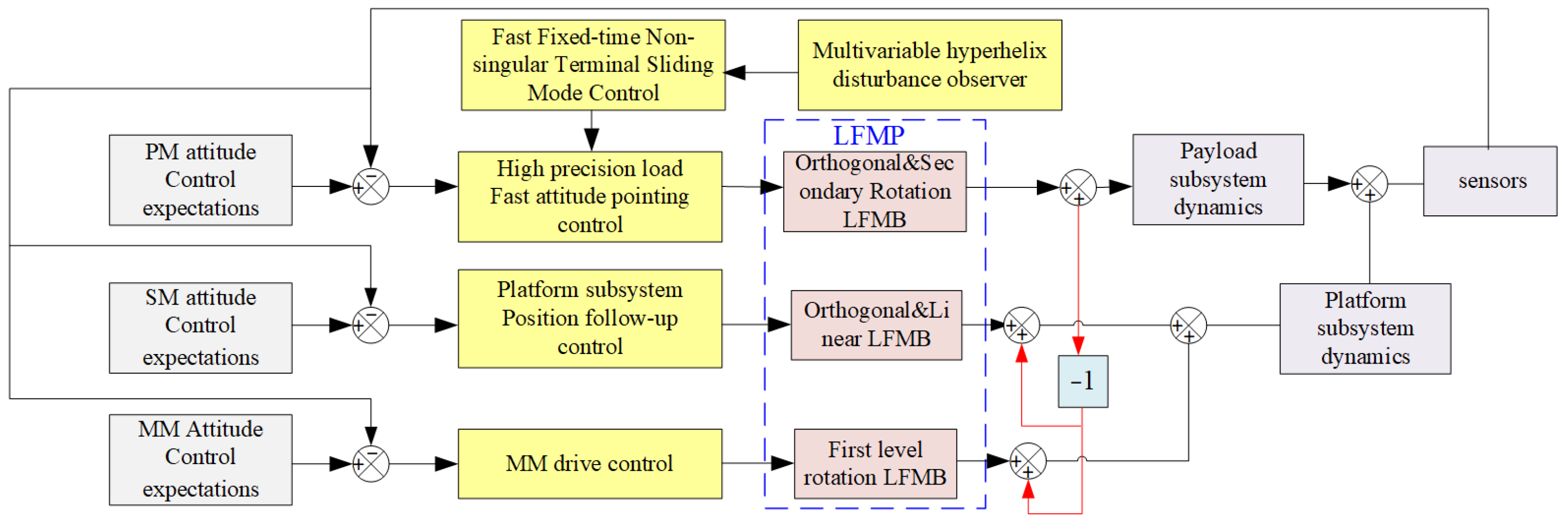
3. Design of Three Body Multi Closed Loop Control Law

The payload-centered control method consists of high-precision rapid attitude pointing of the payload, position tracking of the platform subsystem, and MM tracking. We design a position-tracking control law based on Equation (23), and control the position tracking through a certain allocation strategy using OLFMBs and LLFMBs. On the basis of considering the influence of the position follow-up of the platform subsystem on the coupling of the payload attitude, combined with the theory of multivariable super-twisting, an extended state observer is designed to estimate and compensate for the uncertainty factors of the load attitude. A non-singular fixed-time fast terminal sliding mode surface (NFFTSMS) law is designed, which directly controls the imaging of the satellite load to the ground without additional disturbance force through OLFMBs and two-stage RLFMB, achieving high-precision and fast attitude stability of the payload. Furthermore, considering the interference effect of electromagnetic reactions from OLFMBs and LLFMBs, an MM driving control law is designed based on Equation (26). The specific control scheme is shown in the following Figure 5.
The expected attitude quaternion q p d of the load subsystem and the expected angular velocity ω p d of the load subsystem can be determined by their expected attitude. For the MM and SM, in the load-centered control method, it is necessary to follow the motion of the load subsystem. Therefore, the control objectives of the maglev cabin and satellite platform come from the pose information of the rotating load. If the angle at which the load subsystem rotates around the Y-axis is ϕ , then the quaternion of rotation is q ϕ = q ϕ 0 q ϕ v T T , where q ϕ 0 = cos ϕ / 2 , q ϕ v = 0    sin ϕ / 2    0 T hold.
The expected attitude quaternion of the MM can be expressed as:
q r d = q p q ϕ
where q p is the quaternion of the current attitude of the PM. If the expected angle of rotation of the MM relative to the SM is θ r d , then its expected attitude quaternion is q θ = q θ 0 q θ v T T , where q θ 0 = cos ( θ r d / 2 ) , q θ v = sin ( θ r d / 2 ) 0 0 T hold. The expected attitude quaternion of the satellite platform is:
q b d = q r d q θ *
The attitude transformation matrix of the payload subsystem relative to the expected MM system is denoted as A ϕ . Therefore, the projection ω r d of the expected angular velocity vector of the MM in this system is:
ω r d = A ϕ ( ω p 0 ϕ ˙ 0 T )
The expected position of the centroid of the platform subsystem is:
X p f d = X p + A b d r p f
where X p is the projection of the origin of the payload subsystem in the inertial frame; r p f is the vector pointing from the origin of the MM to the center of mass of the platform subsystem; and A b d is the attitude transformation matrix of the SM relative to the inertial frame.

3.1. Position Follow-Up Control Law of Platform Subsystem

If the position error of the center of mass of the platform subsystem is X p f e = X p f X p f d , then the translational dynamics of the platform subsystem are converted into error form:
X ¨ p f e = X ¨ p f d M p f 1 A b C r F m r
If we define y p f = X p f e + X ˙ p f e , then according to the equation, it can be obtained:
y ˙ p f = X ˙ p f e + X ¨ p f e    = X ˙ p f e X ¨ p f d + M p f 1 F r    = M p f 1 F r + N p f
where F r is the projection of the reaction force of the electromagnetic force applied to the load subsystem by the Lorentz force magnetic levitation bearing in the inertial frame, i.e., F r = A b C r F m r . N p f is the interference term of the position equation, satisfying N p f = X ˙ p f e X ¨ p f d .
The designed linear sliding mode control law is as follows:
F r ( k ) = M p f T p f 1 [ y d ( k + 1 ) y ( k ) 1 ( 1 + T p f α ) e ( k ) ]     + M p f g s s g n ( s ( k ) )
where g s is the parameter of the control law switching term, which has g s > N i ( k ) for any g s . Based on the strategy that minimizes the impact on the attitude of the payload subsystem, the LFMB electromagnetic force distribution scheme for the above control law is formulated as follows:
F u r 1 = ν _ C r T A b T F r F l r 1 = ν _ C r T A b T F r F a r = λ _ C r T A b T F r
where ν _ = d i a g 0.5 0 0.5 , λ _ = d i a g 0 1 0 , F u r 1 , F l r 1 , F a r are the electromagnetic forces for the upper and lower OLFMB and LLFMB, respectively.

3.2. Design of Payload-Centered Attitude Pointing Control Law

Unlike traditional platform-centered control methods, in the payload-centered control method, payload attitude control dominates and changes the direction of control transmission. The payload is not affected by the satellite body and reduces error transmission links. Therefore, it can improve control accuracy and isolate platform vibration effects, achieving a disturbance-free space for payload attitude and providing an ultra-stable and ultra-static working environment. The main differences and comparisons between the two control methods are shown in Table 2.
On the basis of the Equation (28), simplify the attitude dynamics equation of the payload subsystem as follows:
J p l ω ˙ p + ω ˜ p J p l ω p = u p l + D + D 1
where u p l is the attitude control torque of the payload subsystem; D is the interference of the position control force of the platform subsystem on the attitude control of the payload subsystem; and D 1 is the modeling error.
The error quaternion q p e = q p e 0 q p e v T T of the load subsystem can be expressed as:
q p e = q p d * q p
where q p d is the conjugate quaternion of the expected quaternion for the payload subsystem. Definition A ( q p e ) is the attitude transformation matrix of the load system relative to the expected frame, and the error angular velocity ω p e of the load can be expressed as ω p e = ω p ω p r = ω p A ( q p e ) T ω p d . The platform position control force is provided by OLFMBs and LLFMBs:
D = r ˜ s u C p r F u r 1 + r ˜ s a C p r F a r + r ˜ s l C p r F l r 1
Convert the attitude dynamics equation of the payload subsystem into error form:
ω ˙ p e = J p l 1 ( r ˜ s u C p r F u r 1 + r ˜ s a C p r F a r + r ˜ s l C p r F l r 1 ) + J p l 1 D 1 ω ˙ p r + J p l 1 u p l
The kinematic relationship between error quaternion q p e and error angular velocity ω p e is:
q ˙ p e 0 = 1 2 ω p e T q p e v , q ˙ p e v = Q ( q p e ) ω p e
where Q ( q p e ) is a matrix about the error quaternion, satisfying Q ( q p e ) = ( q ˜ p e v + q p e 0 I 3 ) / 2 . Combining Equation (40) and Equation (41), organize the equations as follows:
q ¨ p e v = Q ˙ ( q p e ) ω p e + Q ( q p e ) ω ˙ p e = 1 4 q p e v ω p e T ω p e + Q ( q p e )     ( ω ˙ p r + J p l 1 u p l + J p l 1 ( r ˜ s u C p r F u r 1 + r ˜ s a C p r F a r + r ˜ s l C p r F l r 1 ) + J p l 1 D 1 )
Note that B p = Q ( q p e ) J p l 1 , D p = B p D 1 , therefore the above equation can be organized as:
q ¨ p e v = h p + B p u p l + D p + B p D
h p = 1 4 q p e v ω p e T ω p e Q ( q p e ) ω ˙ p r
Under the influence of unknown bounded interference D p , design a control law u p l so that the system states q p and ω p can track the expected states q p d and ω p d within a fixed time; that is, there exists a time constant T max > 0 , and at t > T max , there are error states q p e v = 0 3 × 1 and ω p e = 0 3 × 1 that hold.
Before designing the control law, provide the following assumptions and related lemmas. For nonlinear systems:
x ˙ = f ( x ( t ) ) , x ( 0 ) = x 0 , f ( 0 n × 1 ) = 0 n × 1
where f : R n R n is a nonlinear function.
Lemma 1
For a system, if there exists a Lyapunov function  V ( x )  with scalars  α 1 ,  β 1 ,  p ,  q ,  k R +  that satisfy  p k < 1  and  q k > 1 , and  V ˙ ( x ) ( α 1 V ( x ) p + β 1 V ( x ) q ) k  holds, then the system is fixed time stable, and its convergence time satisfies the following inequality relationship:
T 1 α 1 k ( 1 p k ) + 1 β 1 k ( q k 1 )
Lemma 2
For scalars  x i R  and  i = 1 , 2 , , n , the following inequality relationship holds for  0 < a 1  and  b > 1 :
i = 1 n x i a i = 1 n x i a , i = 1 n x i b n b 1 i = 1 n x i b
Assumption 1: 
The mass parameters of the payload subsystem are known. In order to estimate the unknown disturbance  D p = B p D 1 , the state variable  x 1 = q ˙ p e v  is defined, and the extended state is  x 2 = D p . Based on the multivariable super-twisting theory, the observer is designed as follows:
Z ˙ 1 = Z 2 λ 1 e 1 e 1 2 1 / 2 λ 2 e 1 e 1 2 ζ 1 + h p + B p u p l + B p D Z ˙ 2 = λ 3 e 1 e 1 2
where  Z 1  and  Z 2  are observation variables,  e 1  is observation error, satisfying  e 1 = Z 1 x 1 ;  λ 1 ,  λ 2 ,  λ 3 , and  ζ  are scalar parameters of the observer, satisfying:
λ 3 > 4 L d , λ 1 > 2 λ 3 , λ 2 > 0 , ζ > 1
where  D 1  is unknown and bounded, and according to  D p = B p D 1  ,  D ˙ p 2 L d  holds.
For unknown bounded interference D p , observer errors e 1 = Z 1 x 1 and e 2 = Z 2 x 2 are defined. When the parameter conditions in the observer satisfy the equation, there exists a finite time T o that makes Z 2 = D p hold for any t T o , where T o satisfies:
T o 1 λ 2 ( ζ 1 ) η ζ 1 + 2 ( 3 η ) 1 / 2 λ 1 + K M × 1 + M m 1 2 λ 3 / λ 1 + 3 K m
where M , m , η , and K are scalar parameters that satisfy: M = λ 3 + L d m = λ 3 L d , η = ( 3 1 / 4 λ 1 / λ 2 ) 1 / ( ζ + 0.5 ) , K e 2 ( 0 ) 2 . Based on the estimation of unknown interference D by the observer, design a non-singular terminal sliding surface s as follows:
s = K ( q p e v ) q p e v + s i g r 2 ( q ˙ p e v )
where K ( q q e v ) is a diagonal matrix. The diagonal element K ( q q e v ) of ( i = 1 , 2 , 3 ) is:
k ( q q e v , i ) = ( a q q e v , i p 1 / ( k r 2 ) + b q q e v , i g 1 / ( k r 2 ) ) k r 2
The sliding surface parameter conditions are a > 0 , b > 0 , k > 1 , 2 > r 2 > 1 , 1 < g k 2 k 1 , and 1 / r 2 < p k < 1 hold. When s = 0 is established, the system states q p e v and q ˙ p e v on the sliding surface converge to the origin within a fixed time S, while q p e 0 and ω p e converge to 1 (or −1) and 0 3 × 1 , respectively: if q p e 0 ( 0 ) > 0 , q p e 0 will converge to 1. If q p e 0 ( 0 ) < 0 , q p e 0 will converge to −1. The convergence time T s satisfies:
T s 2 ( 1 p k ) / 2 a k 3 1 k ( 1 p k ) + 2 ( 1 g k ) / 2 b k 3 1 k ( g k 1 )
Design the NFFTSMS law as follows:
u p l = 1 r 2 B p 1 K ¯ ( q p e v ) + K ( q p e v ) s i g 2 r 2 ( q ˙ p e v ) B p 1 h p    1 r 2 B p 1 d i a g κ ( q ˙ p e v r 2 1 ) d i a g q ˙ p e v 1 r 2    × s i g k 1 ( α s i g p 1 ( s ) + β s i g g 1 ( s ) ) B p 1 ρ s g n ( s )    B p 1 Z 2 D
where k 1 > 1 , 0 < p 1 k 1 < 1 , 1 < g 1 k 1 < 2 k 1 1 , α > 0 , β > 0 and ρ > 0 . κ ( q ˙ p e v r 2 1 ) is a nonlinear function that satisfies:
κ ( x ) = sin ( π x 2 2 τ 2 ) x < τ 1 x τ
where τ is a small enough positive number. In Equation (42), K ¯ ( q p e v ) is the diagonal matrix and the diagonal element k ¯ ( q p e v , i ) ( i = 1 , 2 , 3 ) is:
k ¯ ( q p e v , i ) = k r 2 ( a q p e v , i p 1 / ( k r 2 ) + b q p e v , i g 1 / ( k r 2 ) ) k r 2 1      × ( a ( p 1 k r 2 ) q p e v , i p 1 / ( k r 2 )      + b ( g 1 k r 2 ) q p e v , i g 1 / ( k r 2 ) )
For the error dynamics equation, combining observer, sliding surface, and control law, under the influence of unknown disturbance D p , the error states q p e v and ω p e converge to the origin within a fixed time T , and the upper bound of T satisfies:
T T o + T a + T s
where T o is the convergence time, take K = L m as the solution according to the equation; T a is the convergence time, satisfying:
T a 2 3 1 k 1 α k 1 2 ( p 1 k 1 + 1 ) / 2 ( 1 p 1 k 1 ) + 2 τ 1 / ( r 2 1 ) ρ + 2 3 1 k 1 β k 1 2 ( g 1 k 1 + 1 ) / 2 ( g 1 k 1 1 )
In summary, the satellite platform position tracking control and load attitude control of the load center control method are provided by the electromagnetic force F u r = F u r 1 + F u r 2 of the upper OLFMB, the electromagnetic force F a r of the LLFMB, and the electromagnetic force F l r = F l r 1 + F l r 2 of the lower OLFMB. The load attitude control allocated according to the strategy of no additional disturbance will not affect the force situation of the satellite platform.

3.3. MM Driving Control Law

Convert the driving equation of the frame cabin into error form:
θ ¨ r e = θ ¨ r d J r x 1 ω ˙ b T R r D r J r x 1 ω b T R ˙ r D r    J r x 1 D r T r ˜ r u F u r + r ˜ r a F a r + r ˜ r l F l r + J r x 1 τ r a
In the formula, r ˜ r u F u r , r ˜ r a F a r , and r ˜ r l F l r reflect the interference effects of the position follow-up control force of the platform subsystem and the attitude control force of the payload subsystem on the drive control of the MM. Design control torque τ r a so that the error states θ r e and θ ˙ r e are zero, that is, states θ r and θ ˙ r track the expected states θ r d and θ ˙ r d . The design control law is as follows:
τ r a = J r x θ ¨ r d + ω ˙ b T R r D r + ω b T R ˙ r D r + D r T r ˜ r u F u r + r ˜ r a F a r + r ˜ r l F l r K k θ r e D k θ ˙ r e
where K k and D k are the proportional control parameters and differential control parameters for the frame cabin attitude, respectively.

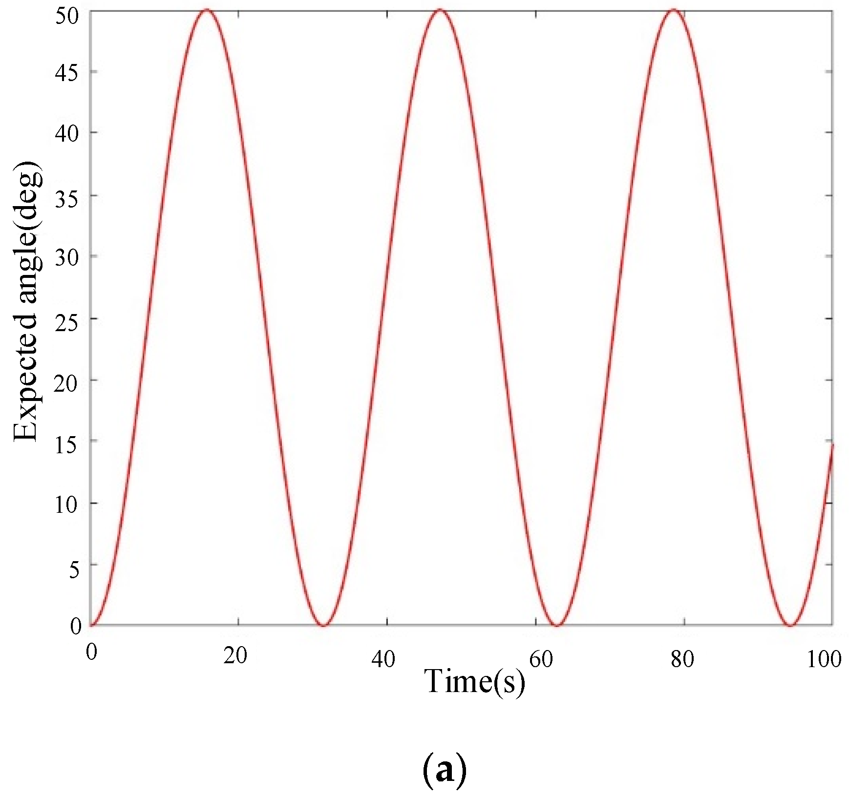
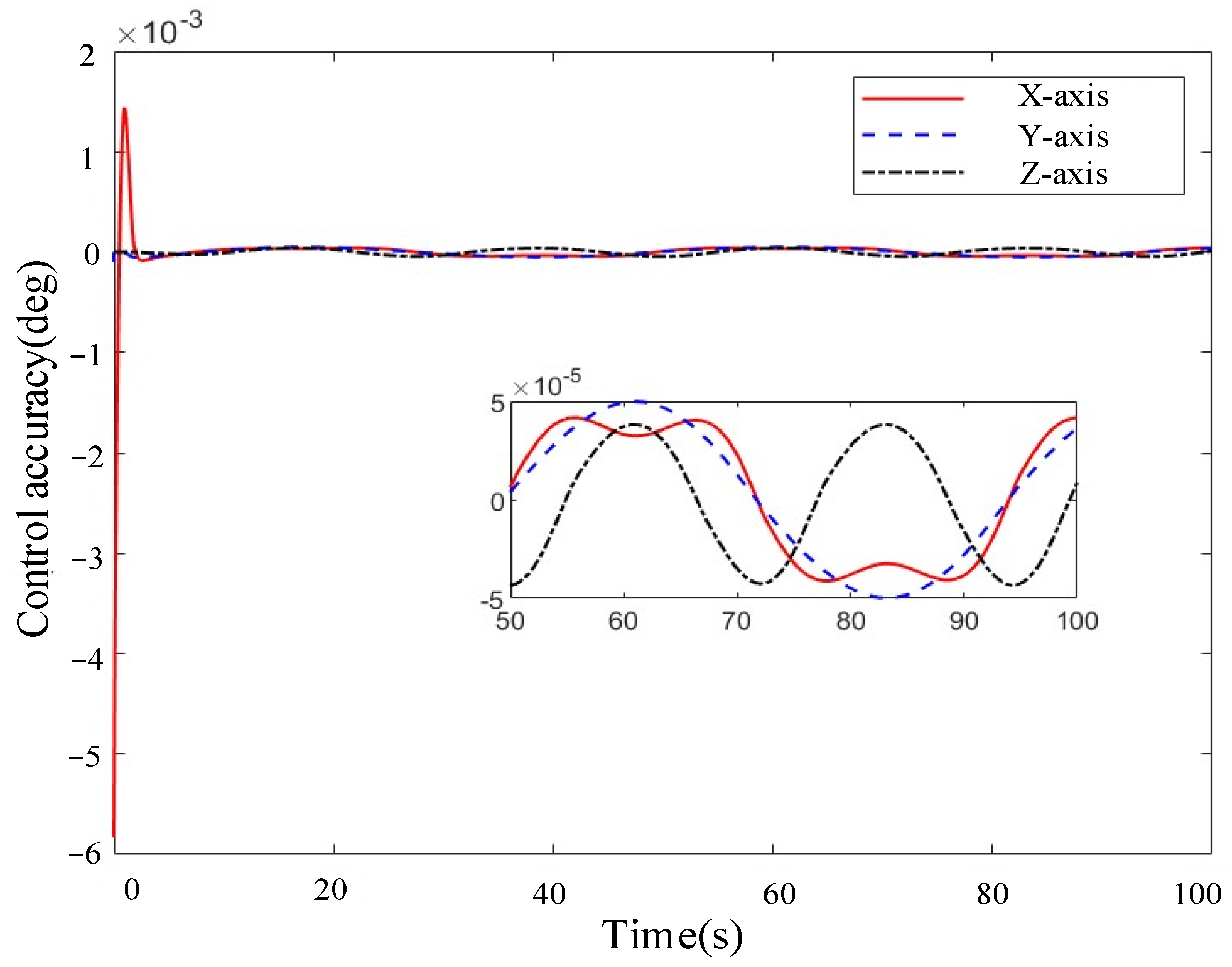
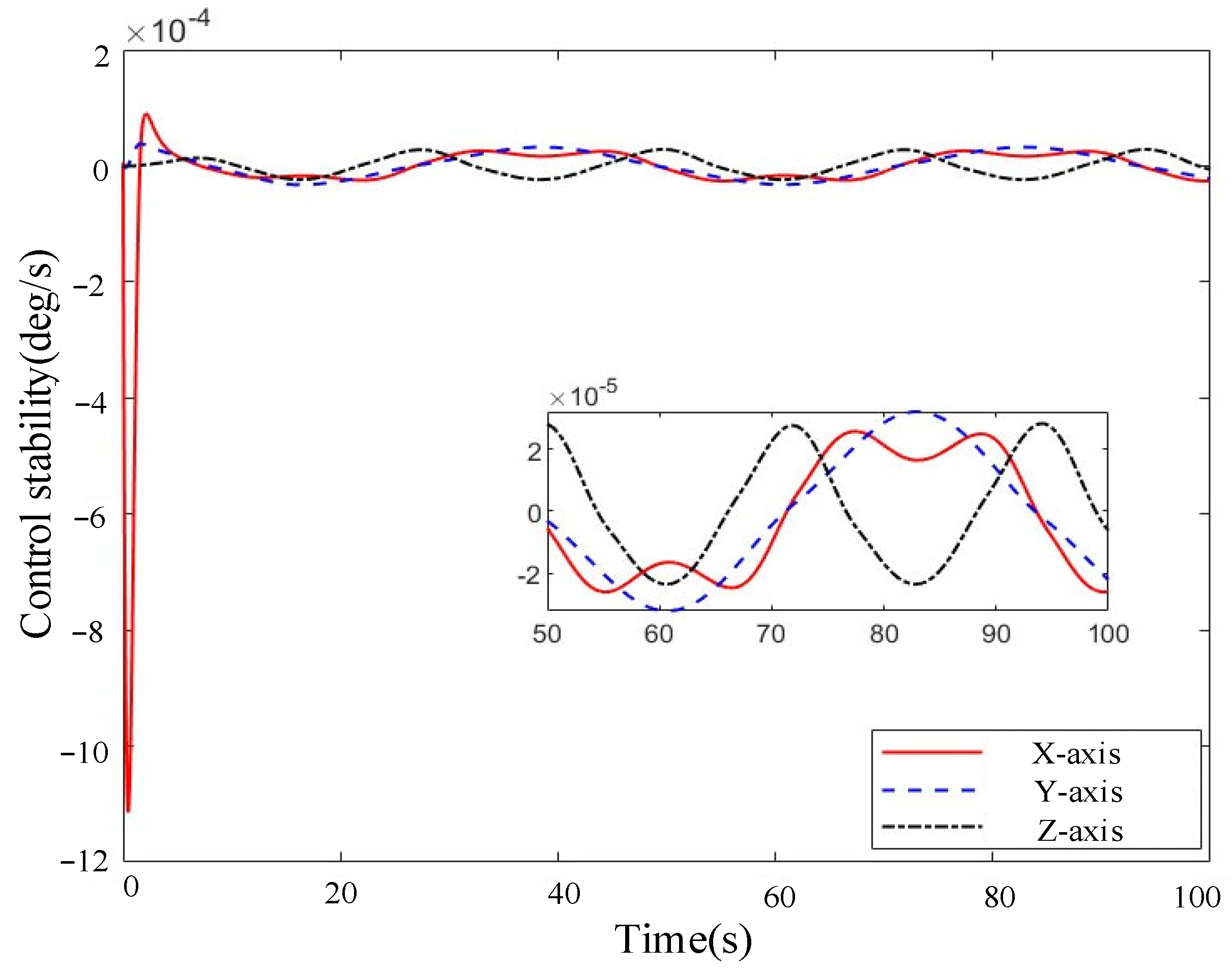
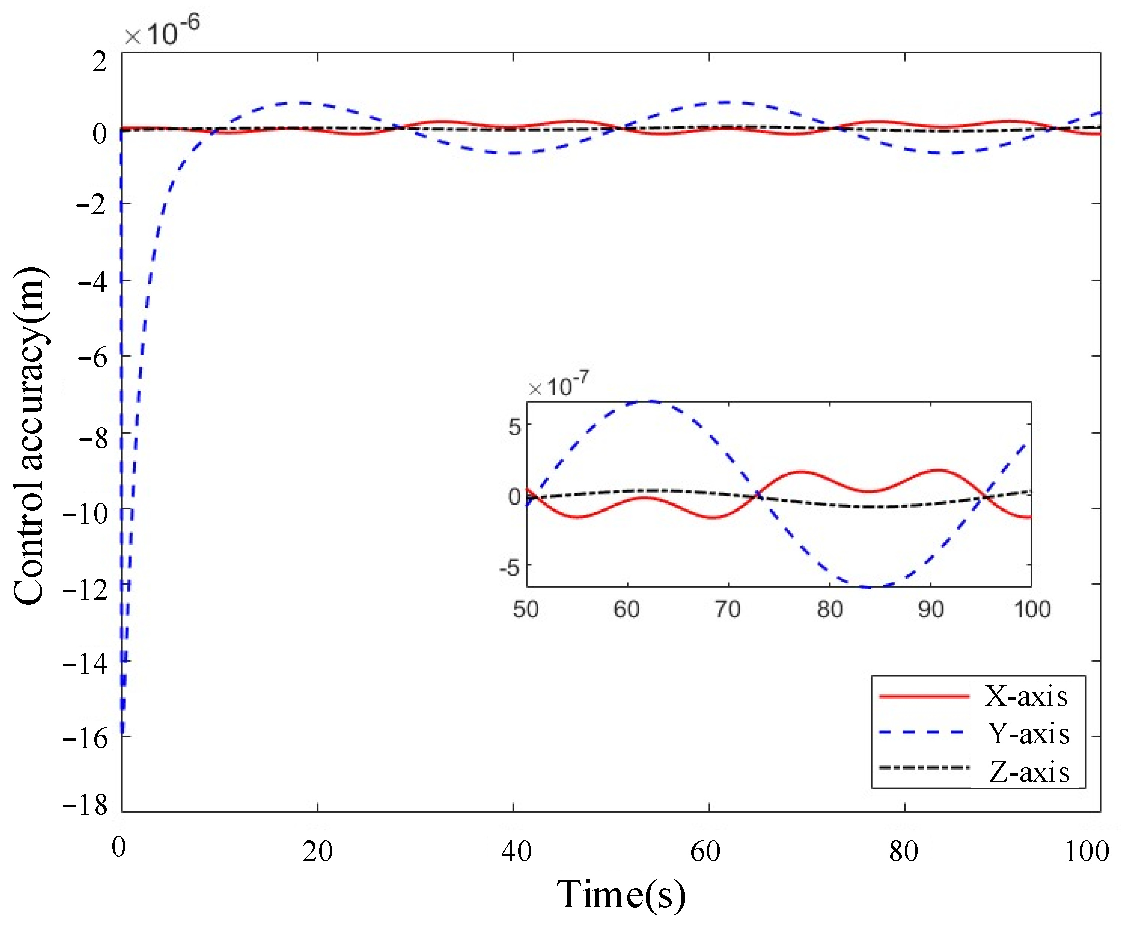
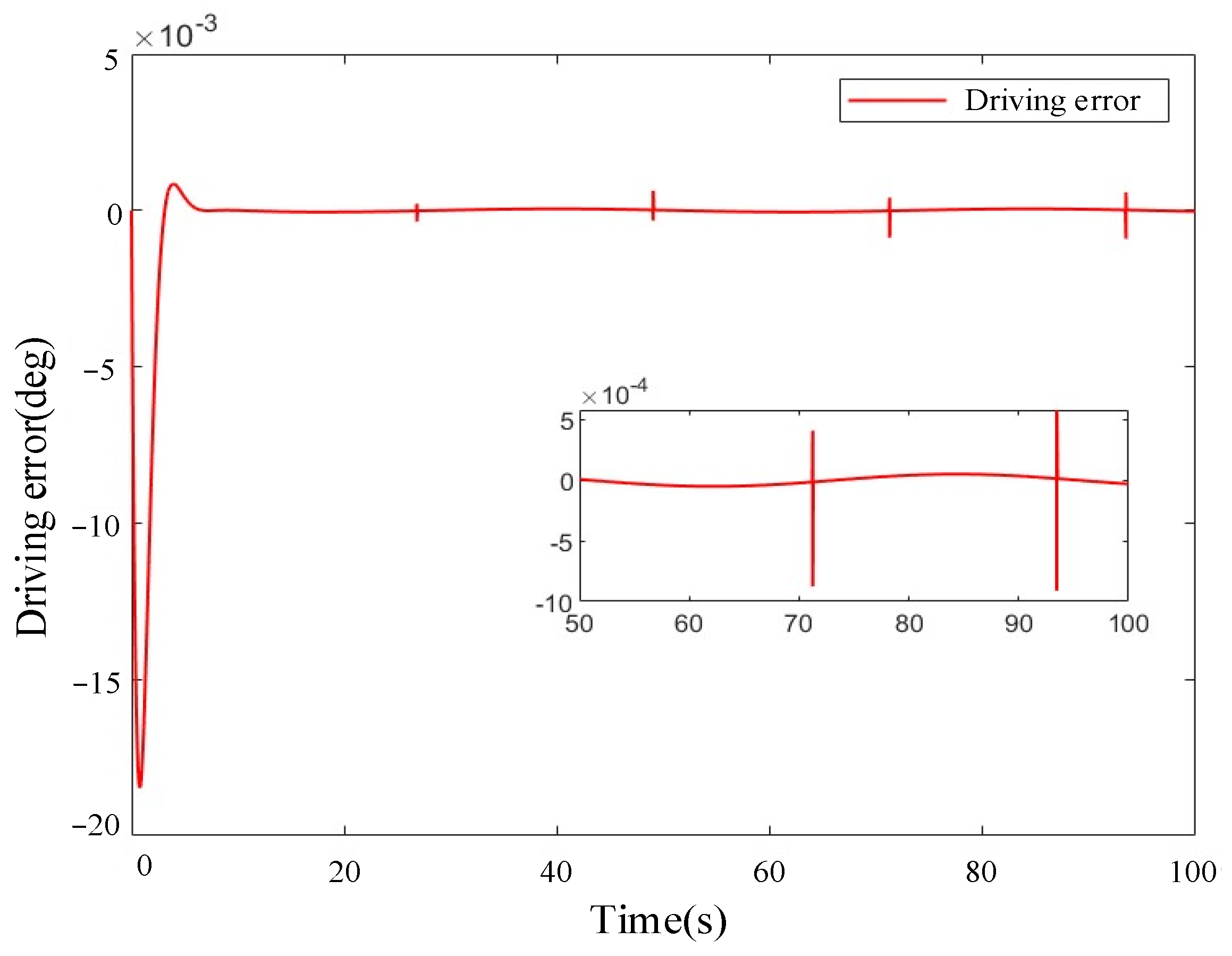
4. Simulation Results and Analysis

This chapter conducts simulation analysis on the pointing accuracy, pointing stability, dynamic tracking ability, and in-orbit bearing capacity of the Lorentz force magnetic levitation gimbal stabilization platform. It verifies the advantages of payload-centered control methods in improving the accuracy of imaging load control and isolating satellite body vibration, thereby verifying the effectiveness of the proposed high-precision fast attitude pointing control algorithm for imaging loads. The mass parameters of the LFMP are shown in Table 3.
Set the initial angular velocity of the satellite platform to ω b ( 0 ) = 0.001 0 0 T   r a d / s . Set the initial value of imaging load angular velocity to ω p ( 0 ) = 0.001 0 0 T   r a d / s . The expected motion of the payload subsystem is to rotate along its own axis while following the X-axis rotation of the MM at an orbital angular velocity of ω 0 = 0.0011   r a d / s . The reference controller parameters are shown in Table 4 below.
Conduct attitude control simulation on the LFMP without considering the elastic vibration of the solar wing and the rapid maneuvering of the payload subsystem.
The axial rotation of the payload subsystem and the control expectation of the MM are shown in Figure 6. The control limit for the position control force of the platform subsystem is set to 0.1 N, the control limit for the payload attitude control torque is set to 0.1 Nm, and the control limit for the payload attitude control force is set to 0.1 N. The control limit for the driving torque of the MM is set to 0.1 Nm.
According to Figure 7 and Figure 8, the attitude accuracy of the payload subsystem is 0.00002°, and the attitude stability is within 0.00005°/s.
According to Figure 9, the position control accuracy is 0.0000005 m. According to Figure 10, the driving error of the MM is 0.001°.
It can be seen that in the payload-centered control method, the payload subsystem has higher accuracy and smoother motion compared to the platform subsystem. This verifies the advantage of the payload-centered control algorithm in improving the accuracy of payload imaging control, and further verifies the effectiveness of the high-precision fast attitude pointing control algorithm for imaging payloads.

5. Conclusions

The high-precision fast attitude pointing control method centered on the payload can achieve the control goal of “active payload, platform follow-up”, reduce the transmission of imaging payload errors, and isolate the impact of satellite body vibration. An evaluation of the stability with a specific model mentioned earlier has been performed. The attitude accuracy of the payload subsystem is 0.00002° and the attitude stability is within 0.00005°/s, achieving ultra-high precision, ultra-high stability, and ultra-high agility attitude pointing control of imaging payloads. The payload-centered control method is also applicable to precise attitude control of other non-contact isolation systems, except for the specific model proposed in this paper.

Author Contributions

Writing—original draft preparation, Z.L.; writing—review and editing, W.W.; visualization, Z.L.; supervision, L.W.; project administration, W.W.; funding acquisition, W.W. All authors have read and agreed to the published version of the manuscript.

Funding

This research was funded by the National Natural Science Foundation of China, grant number 52075545.

Institutional Review Board Statement

Not applicable.

Informed Consent Statement

Not applicable.

Data Availability Statement

The data presented in this study are available on request from the corresponding author due to the research project involved in the article involves relevant confidentiality agreements, and the overall project has not been completed yet.

Conflicts of Interest

The authors declare no conflict of interest.

References

  1. Liu, L. Research on Active Vibration Isolation and Precise Directional Control Technology for Spacecraft. Ph.D. Thesis, Harbin Institute of Technology, Harbin, China, 2011. [Google Scholar]
  2. Liu, Q.; Wang, K.; Ren, Y.; Peng, P.; Ma, L.; Yin, Z. Novel repeatable launch locking/unlocking device for magnetically suspended momentum flywheel. Mechatronics 2018, 54, 16–25. [Google Scholar]
  3. Kalenova, V.I.; Morozov, V.M. Novel approach to attitude stabilization of satellite using geomagnetic Lorentz forces. Aerosp. Sci. Technol. 2020, 106, 106101–106105. [Google Scholar] [CrossRef]
  4. Zhu, H.; Teo, T.J.; Pang, C.K. Flexure-Based Magnetically Levitated Dual-Stage System for High-Bandwidth Positioning. IEEE Trans. Ind. Inform. 2019, 15, 4665–4675. [Google Scholar] [CrossRef]
  5. Labib, M.; Piontek, D.; Valsecchi, N.; Griffith, B.; Dejmek, M.; Jean, I.; Mailloux, M.; Palardy, R.; Michels, J.; Michalyna, C.; et al. The Fluid Science Laboratory’s Microgravity Vibration Isolation Subsystem Overview and Commissioning Update. In Proceedings of the SpaceOps 2010 Conference Delivering on the Dream, Huntsville, AL, USA, 25–30 April 2010; pp. 443–452. [Google Scholar]
  6. Basovich, S.; Arogeti, S.A.; Menaker, Y.; Brand, Z. Magnetically Levitated Six-DOF Precision Positioning Stage with Uncertain Payload. IEEE/ASME Trans. Mechatron. 2016, 21, 660–673. [Google Scholar] [CrossRef]
  7. Dyck, M.; Lu, X.; Altintas, Y. Magnetically Levitated Rotary Table with Six Degrees of Freedom. IEEE/ASME Trans. Mechatron. 2017, 22, 530–540. [Google Scholar] [CrossRef]
  8. Ahn, D.; Jin, J.; Yun, H.; Jeong, J. Development of a Novel Dual Servo Magnetic Levitation Stage. Actuators 2022, 11, 147. [Google Scholar] [CrossRef]
  9. Li, Z.F.; Liu, Q.; Ren, W.J. Dynamic modeling of active vibration isolation systems with high and micro gravity in space. Vib. Shock. 2010, 29, 1–4. [Google Scholar]
  10. Zhang, W.; Zhao, Y.B.; Liao, H.; Zhao, H.B. Design of a dual hypersatellite platform with dynamic and static isolation and master-slave collaborative control. Shanghai Aerosp. 2014, 31, 7–11. [Google Scholar]
  11. Zhao, J.; Yang, F. Technological Innovation and Application Practice of China’s High Resolution Agile Small Satellites. Spacecr. Eng. 2021, 30, 23–30. [Google Scholar]
  12. Yaseen, H.M.S.; Siffat, S.A.; Ahmad, I.; Malik, A.S. Nonlinear adaptive control of magnetic levitation system using terminal sliding mode and integral backstepping sliding mode controllers. ISA Trans. 2022, 126, 121–133. [Google Scholar] [CrossRef] [PubMed]
Figure 1. Structure diagram of maglev satellite.
Applsci 14 07588 g001
Figure 2. A multi-body dynamic modeling scheme for LMFPs.
Applsci 14 07588 g002
Figure 3. Coordinate system definition diagram.
Applsci 14 07588 g003
Figure 4. Position vector definition diagram.
Applsci 14 07588 g004
Figure 5. Three-body High-precision attitude control scheme centered on payload.
Applsci 14 07588 g005
Figure 6. Control expectations. (a) Expected angle; (b) expected angular velocity; (c) expected angular acceleration.
Applsci 14 07588 g006aApplsci 14 07588 g006b
Figure 7. Attitude accuracy of payload subsystem.
Applsci 14 07588 g007
Figure 8. Attitude stability of payload subsystem.
Applsci 14 07588 g008
Figure 9. Platform subsystem position control accuracy.
Applsci 14 07588 g009
Figure 10. Error in driving control of MM.
Applsci 14 07588 g010
Table 1. Position vector definition.
SymbolicSignificance
X ¯ p f The origin of the inertial frame points towards the center of mass of the platform subsystem
r ¯ b The centroid of the platform subsystem points to a certain quality element on the platform
r ¯ r The center of mass of the platform subsystem points towards the origin of the MM
g ¯ r The origin of the MM system points to a certain mass element of the MM
Table 2. Comparison of two control methods.
CategoryPlatform-Centered Control MethodPayload-Centered Control Method
Payload attitude control expectationExpected trajectory undergoes two-stage rotationOn the basis of ground orientation, two-stage rotation according to the expected trajectory
Payload measuring elementNon-contact eddy current sensorStar sensors, gyroscopes, and position sensors
Satellite platform control expectationsGround orientation (only unilateral posture)Follow the movement of the payload (in terms of position and posture)
Table 3. LFMP Parameters.
CategoryCentroid Position/Attitude QuaternionQuality (kg)Moment of Inertia (kg × m2)
Satellite [ 0 , 0 , 0.46977 ] , [ 1 , 0 , 0 , 0 ] 276 50 0 0 0 60 0 0 0 60
Payload [ 0 , 0 , 0 ] , [ 1 , 0 , 0 , 0 ] 15 1 0 0 0 1 0 0 0 1
SM [ 0.00538 , 0.00781 , 0.18687 ] , [ 1 , 0 , 0 , 0 ] 26.14 0.287 7.75 × 10 7 0.016 7.75 × 10 7 0.269 0.029 0.016 0.029 0.41
MM [ 0 , 0 , 0 ] , [ 1 , 0 , 0 , 0 ] 10.954 0.016 1.01 × 10 5 1.34 × 10 5 1.01 × 10 5 0.029 6.20 × 10 7 1.34 × 10 5 6.20 × 10 7 0.021
PM [ 0 , 0 , 0 ] , [ 1 , 0 , 0 , 0 ] 1.7599 0.0021 8.48 × 10 11 6.46 × 10 10 8.48 × 10 11 0.0019 2.79 × 10 7 6.46 × 10 10 2.79 × 10 7 0.0037
Table 4. Reference controller parameters.
ParametersValuesParametersValues
g s 2 × 10 4 ζ 1.5
K k 15 λ 1 0.01001
D k 1 g 0.7
L 0.00001 m k 2
λ 2 0.00001 a 1.5
p 0.4975 p 1 0.5
r 2 1.01 k 1 1.85
b 1.5 β 0.5
g 1 1.35 δ s 0.0001
α 0.5 ρ 0.00001
τ 0.005
Disclaimer/Publisher’s Note: The statements, opinions and data contained in all publications are solely those of the individual author(s) and contributor(s) and not of MDPI and/or the editor(s). MDPI and/or the editor(s) disclaim responsibility for any injury to people or property resulting from any ideas, methods, instructions or products referred to in the content.

