Abstract
Surgeons face a significant challenge due to the heat generated during drilling, as excessive temperatures at the bone–tool interface can lead to irreversible damage to the regenerative soft tissue and result in thermal osteonecrosis. While previous studies have explored the use of machine learning to predict the temperature rise during bone drilling, this in vitro study introduces a comprehensive approach by combining the Response Surface Methodology (RSM) with advanced machine learning techniques. The main objective lies in the comprehensive evaluation and comparison of support vector machine (SVM) and random forest (RF) models specifically for the optimization of the bone drilling parameters to prevent thermal bone necrosis. A total of 27 experiments were conducted using a multi-level factorial method, with analysis performed via the Minitab software version 19.1. Performance metrics such as the mean squared error (MSE), mean absolute percentage error (MAPE), and coefficient of determination (R2) were used to assess model accuracy. The RF model emerged as the most effective, with R2 values of 94.2% for testing and 97.3% for training data, significantly outperforming other models in predicting temperature fluctuations. This study demonstrates the superior predictive capabilities of the RF model and offers a robust framework for the optimization of surgical procedures to mitigate the risk of thermal damage.
1. Introduction
Bone drilling is an essential procedure in orthopedic surgery, dental implant placement, and other medical interventions that involve the insertion of screws, plates, or prostheses into the bone [1]. However, one of the significant challenges with bone drilling is the generation of excessive heat, which can lead to a phenomenon called thermal osteonecrosis. Thermal osteonecrosis refers to the death of bone cells (osteocytes) due to elevated temperatures [2,3].
The consequences of thermal osteonecrosis are far-reaching. The affected bone areas may become weakened, leading to poor implant integration, prolonged healing times, or increased susceptibility to post-operative infections [4]. For surgeries that demand robust bone healing, like fracture repairs or spinal fusions, thermal osteonecrosis can even lead to treatment failure [5,6]. Thermal osteonecrosis can be managed by optimizing the operation of the surgical drilling system [7]. Achieving this often necessitates precise predictions, such as estimating the bone drilling temperature based on the optimal combination of the drilling parameters.
The field of machine learning provides efficient techniques for the prediction of bone drilling temperatures based on data [8]. As a branch of computer science, machine learning focuses on how computers can learn autonomously without being directly programmed with specific rules. It encompasses two primary areas: supervised learning and unsupervised learning [9,10]. In supervised learning, predictive models are developed using labeled data, involving tasks like predicting drilling temperatures through regression. Conversely, unsupervised learning deals with unlabeled data and is often utilized for tasks such as outlier detection through clustering [11].
Machine learning techniques are increasingly employed in the modern Industry 4.0 to forecast uncertainty and manage vast amounts of data. Pandey and Panda [12] used machine learning models to alleviate drilling-induced damage to bovine bone. Akgundogdu et al. [13] utilized machine learning methods to evaluate the bone characteristics and categorize different specimens. Support vector machine (SVM) techniques have demonstrated significant success in characterizing the rigidity of trabecular bone samples. Lu et al. [14] implemented machine learning models to improve the anticipation of postsurgical facial profiles using video imaging. Agarwal et al. [15] conducted a comparison of various machine learning models to predict the mechanical strength of orthopedic bone screws, while Agarwal et al. [16] confirmed different assumptions regarding the use of machine learning models in forecasting thermal injuries. Torun and Öztürk [17] employed machine learning models for robotic bone drilling, noting the effectiveness of closed-loop signals in detecting drill bit damage and the morphology during sheep femur bone drilling.
The aim of developing predictive models is to create models that can accurately predict new data that are not available during their creation [18]. A model trained on a specific dataset cannot be evaluated on the same dataset because it retains a “memory” of it. Therefore, the entire dataset is typically split into two parts: one for the training of the model, known as the training set, and the other for the evaluation of the model, known as the test set. This approach allows for the estimation of the model’s generalization capabilities, indicating how well it will perform on unseen data. It is crucial to ensure that no information from the test set leaks into the training set when developing predictive models. Models built with training sets containing test set information will produce overly optimistic results.
The experiment was designed and optimized using the Response Surface Methodology (RSM) technique. The collected data were analyzed to develop two predictive models for the temperature increase using the support vector machine (SVM) and random forest (RF) methods. The main purpose of these models was to improve the evaluation of bone workability. Therefore, the research objectives of this study were as follows.
- To investigate the crucial machinability factors affecting the bone drilling process, with a particular emphasis on the temperature distribution. By exploring the thermo-mechanical properties of these factors, we aim to enhance our understanding and improve the efficiency of bone drilling procedures.
- To evaluate the performance of bovine bone under varying machining conditions, specifically focusing on the effects of the spindle speed, feed rate, and drill bit diameter. Additionally, we seek to analyze the thermo-mechanical interactions occurring during the drilling process.
- To enhance the machining parameters and determine the best combinations of the spindle speed, feed rate, and drill bit diameter to reduce thermal osteonecrosis in bone by utilizing the Response Surface Methodology (RSM).
- To deploy ML models, particularly random forest (RF) and support vector machine (SVM), to forecast the highest temperature increase. To assess the model’s accuracy and performance in predicting the machining results based on the input variables and confirm the precision and dependability of the ML models.
2. Materials and Methods
The thermal and mechanical characteristics of fresh bovine bone are uniform and closely mimic those of human bone [19,20]. The preparation process for the experimental bone drilling involving bovine femur specimens is shown in Figure 1. The epiphysis (end) of the fresh femur was removed using a saw. Subsequently, the diaphysis (middle part) was chosen for experimentation [21,22], and the periosteum, which is the soft tissue attached to the outer cortical bone, was eliminated to prevent the obstruction of the drill bit’s flute, as recommended in previous studies [23,24,25,26]. Specimens with a cortical thickness exceeding 8 to 13.2 mm were selected for inclusion in the study [27,28].
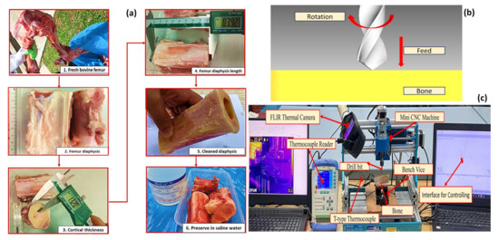
Figure 1.
(a) Bone specimen preparation, (b) schematic diagram of drilling, and (c) cortical bone drilling experimental setup.
This investigation used bovine femur bone as the study material because human bone was not accessible. Bovine bone is considered the closest analog to human bone in terms of its properties. The femoral bone from cattle was obtained promptly after slaughter from a local slaughterhouse. The bone specimens were stored in saline water at −20 °C to preserve their mechanical and thermo-physical properties, and the experiments were conducted within a few days of procurement.
The machinability study was performed with a radial drilling machine, employing a high-speed steel (HSS, Bosch, Petaling Jaya, Malaysia) drill bit with a standard cutting point head geometry of 118°. The temperature readings were recorded using a multi-channel temperature meter connected to a T-type thermocouple [29,30]. The data were stored in an external storage repository. The bone workpiece was firmly fixed in a vice, and various process parameters, as outlined in Table 1, were selected. The input variables considered in this research were the spindle speed, feed rate, and drill bit diameter, while the response variable measured was the elevated average maximum temperature.

Table 1.
Process parameters used in the experiment.
2.1. Response Surface Methodology
The Response Surface Methodology (RSM) is a set of mathematical and statistical techniques designed for the modeling and analysis of problems where multiple variables influence a response variable, with the primary goal being to optimize this response [31,32]. Minitab, a statistical software program, provides robust tools for the performance of the RSM. The first step in the RSM is to design experiments that yield sufficient data to model the response surface, using designs such as central composite designs (CCD) and Box–Behnken designs (BBD). Once the data from these experiments are collected, the next step is to fit a polynomial model, typically a second-order (quadratic) model, to the data. This model can be expressed as in Equation (1):
where is the response variable, and are the input variables, is the intercept, is the linear coefficient, is the quadratic coefficient, is the interaction coefficient, and is the error term. Minitab uses regression analysis to estimate the coefficients of this polynomial model, which includes performing an analysis of variance (ANOVA) to determine the significance of the model and individual predictors, as well as a lack-of-fit test to check the model’s fit to the data. After fitting the model, Minitab generates response surface plots and contour plots to visualize the relationships between the input factors and the response. These plots aid in understanding how changes in the input variables affect the response and help to identify optimal conditions. The final step is to find the optimal settings of the input variables that maximize or minimize the response. Minitab’s optimization tool uses the fitted model to identify these settings, often by solving the optimization problem using Equation (2):
2.2. Support Vector Machine for Regression (SVR)
Support vector regression (SVR) is a nonlinear regression method based on support vector machines (SVM) [33,34]. It aims to construct a hyperplane that reduces the prediction errors and maximizes the margin between the hyperplane and the closest data points. An epsilon tube is used to define acceptable error boundaries. The algorithm applies a kernel function to project the input data into a higher-dimensional feature space, allowing for the creation of the hyperplane and the minimization of errors in this new space. The structure of SVM regression is illustrated in Figure 2.
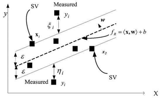
Figure 2.
The framework of support vector machine regression.
SVR can be expressed as a convex optimization problem according to Equation (3). Convex optimization ensures that any local minimum is a global minimum, simplifying the task of determining the optimal hyperplane. The optimization problem aims to minimize the error within a specified margin of tolerance, often incorporating a regularization term to prevent overfitting.
where represents the classes, and denotes a set of features. The parameter b corresponds to the width of the hyperplane, and W signifies the margin. To handle situations where the constraints become infeasible, slack variables and are introduced. The parameter C is used to achieve a trade-off between the width of the margin and the degree of misclassification, effectively controlling the balance between achieving a wider margin and allowing some errors in classification. The process of building an SVM can be visualized through the flow chart presented in Figure 3, which outlines the steps involved in training and predicting the model.
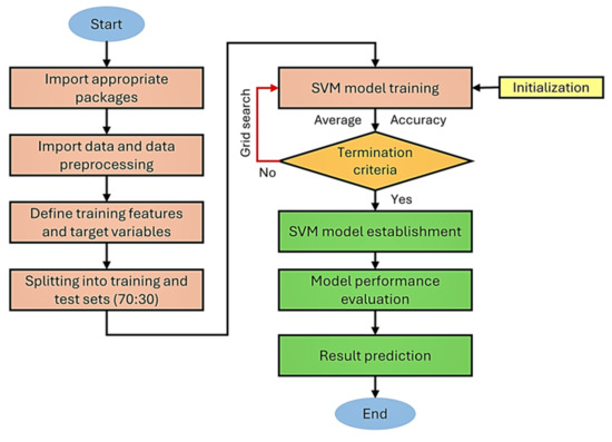
Figure 3.
Flow chart for the implementation process of a support vector machine.
SVR finds application in various fields requiring continuous value predictions, such as financial forecasting, time-series prediction, and other domains necessitating robust regression analysis. Understanding SVR requires a solid grasp of the basic concepts of machine learning, optimization, and linear algebra. This technique is powerful because of its ability to handle high-dimensional data and provide accurate predictions.
2.3. Random Forest Regression (RFR)
Random forest regression (RFR) is a supervised learning algorithm that falls within the ensemble learning family and is utilized for tasks such as regression and classification [35]. During the training phase, numerous decision trees are created. Each decision tree in the forest is constructed using a random subset of the training data and features, promoting diversity and reducing overfitting. The final output from RFR is obtained by averaging the predictions made by each tree, which enhances the accuracy and robustness. This method capitalizes on the strengths of multiple models to produce a more reliable and stable prediction compared to a single decision tree, as shown in Figure 4. RFR is widely favored for its simplicity, versatility, and superior performance in handling complex datasets and capturing non-linear relationships.
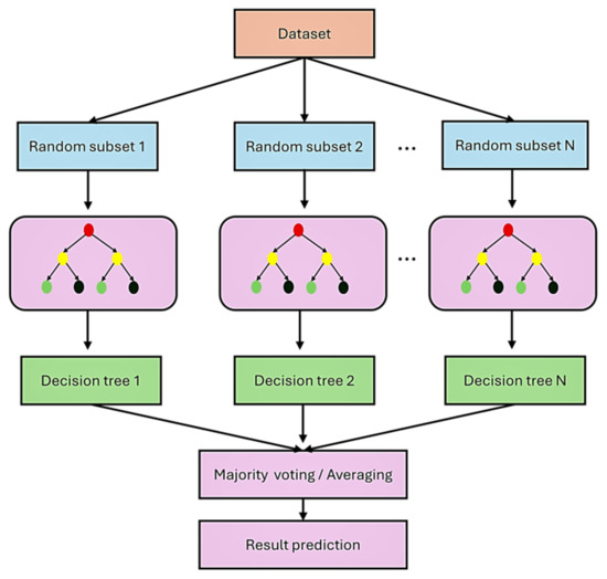
Figure 4.
Illustration of random forest construction.
2.4. Data Pre-Processing and Performance Evaluation Metrics
The experimental data, capturing the average maximum temperatures recorded during bone drilling at three distinct parameter levels, were imported into Google Colab using the Pandas Python library (version 3.10.12). Pandas is widely used for its robust capabilities in data manipulation, enabling the efficient handling and analysis of complex datasets.
The SVM and RF models’ performance was evaluated using standard metrics for model assessment, namely the mean squared error (MSE), mean absolute percentage error (MAPE), and coefficient of determination (R2), described by the following equations:
where n denotes the quantity of data points, represents the observed values, stands for the predicted values, and denotes the mean value of y.
3. Results and Discussion
In optimization, the Design of Experiments (DOE) plays a pivotal role in systematically planning and conducting experiments. By doing so, the DOE ensures that the data collected are reliable and meaningful, which helps in drawing valid conclusions. This methodology reduces the necessity for a large number of experiments, which can be resource-intensive, time-consuming, and costly, while still maintaining high levels of precision in the results.
The accuracy of the results is a key consideration in this context. Ensuring accuracy means that the outcomes of the experiments are not only precise but also reflect the true effects of the variables being studied. This is where the Response Surface Methodology (RSM) becomes particularly valuable. The RSM is a set of statistical and mathematical techniques that are used to model and analyze problems where multiple variables influence the responses. For instance, in medical applications, regarding the drilling temperature of bone during surgery, the RSM can be used to model how different factors (like the spindle speed, feed rate, and drill bit diameter) affect the temperature. By analyzing these factors, researchers can optimize the drilling process to minimize the thermal damage to the bone, thereby improving the surgical outcomes and patient recovery.
A total of 27 experiments were performed utilizing the multi-level factorial method, as shown in Table 2, with the Minitab software aiding in the analysis. Figure 5a illustrates the drilled holes within the bone and Figure 5b shows the schematic diagram of the thermocouple location. The temperature during the drilling process was continuously monitored using a T-type thermocouple, capable of measuring temperatures from 0 to 260 °C, and recorded with an Appellant AT4808 multi-channel thermometer data logger (Applent Instruments, Changzhou, China). The results from these experiments are summarized in Table 2.
Table 2.
Temperature observed in case of drilling bovine bone.
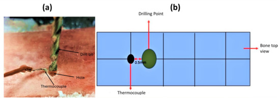
Figure 5.
(a) Illustration of bone drilling site and (b) schematic diagram of thermocouple location from the drilling site.
3.1. Optimization Using RSM
The Response Surface Methodology (RSM) optimization technique was implemented to determine the optimal combination of input variables, such as the spindle speed, feed rate, and drill diameter, which resulted in the lowest feasible process temperature. Figure 6 illustrates the optimization procedure that was designed to consider the model’s predicted minimum process temperature and desirability constraints. The red color represents the optimization input, the blue color indicates the predicted outcome of the experiment, and the black dots correspond to the level of each parameter as shown in Figure 6. The results of the validation process, which encompass a thorough comparison with the experimental data, are comprehensively presented in Table 3. Notably, the model exhibits a remarkably low error rate of just 0.45%, underscoring its exceptional accuracy and reliability.
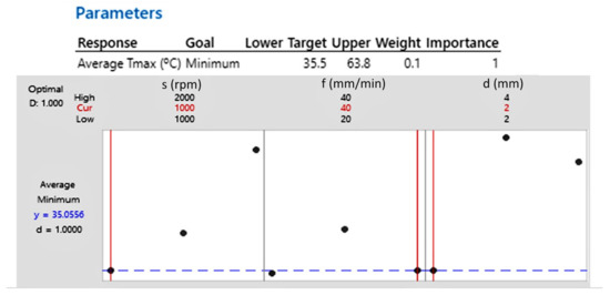
Figure 6.
Input parameter optimization to achieve minimum response temperature.
Table 3.
Optimization to achieve the lowest temperature.
Within the studied range of input values, the process temperature can be reduced to a minimum of 35.05 °C. The most favorable outcomes were achieved using a tool diameter of 2 mm, a feed rate of 40 mm/min, and a rotation speed of 1000 rpm. As shown in Figure 6, a comprehensive array of adjustable input parameters is available to ensure that the temperature applied to the bone remains safe, effectively minimizing the risk of damage to the bone tissue.
3.2. Prediction of Response Variables by SVM and RF
In this research, two distinct regression-based machine learning models were employed to forecast the response values derived from a bone drilling procedure. The dataset was divided randomly, with 70% allocated for model training and the remaining 30% for testing and validation purposes. The models utilized three key input variables—the spindle speed, feed rate, and drill bit diameter—to predict the temperature generated during drilling. To mitigate potential errors arising from differences in the units of these input parameters, both the training and testing datasets were normalized using one-hot encoding. Furthermore, cross-validation was conducted to evaluate and optimize the models by employing a grid search CV to guarantee the selection of the most appropriate parameters while simultaneously considering both training and testing errors.
The temperature values for bone drilling were derived from 27 experiments utilized for both training and testing. Table 4 displays the varied predictions from the support vector regression (SVR) and random forest regression (RFR) models. Table 5 lists the testing and training errors, assessed using three performance indicators to gauge the prediction accuracy.
Table 4.
Predicted bone drilling temperature values from different machine learning algorithms.
Table 5.
Performance metrics for different machine learning algorithms.
3.3. Comparison of Machine Learning and RSM Models
The precision and resilience of both the machine learning and standard RSM predictive models were assessed utilizing three distinct error metrics: MSE, MAPE, and R2. A comparison of these metrics is presented in Figure 7. It was noted that the machine learning predictive model (RFR) demonstrated superior error metrics in comparison to the standard RSM model. Thus, one can deduce that the RFR model is the most resilient and appropriate predictive model for the forecasting of the temperature during bone drilling.
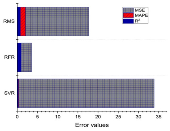
Figure 7.
Error metrics in the context of machine learning models compared to the Response Surface Methodology (RSM) model.
The spindle speed was deemed crucial for all outcomes. It was noted that the rise in the drill bit diameter led to an increase in the temperature caused by drilling as the helicoid formation deepened and expanded. In contrast, the temperature declined as the feed rate rose. Ein-Afshar et al. [36] documented similar discoveries while examining the drilling procedure on bone. The presence of non-uniform structures in bone samples presents obstacles in attaining uniform surface smoothness and a consistent temperature rise along the entire length of a bored hole. The cutting operation had a notable impact on the adjacent tissue of the bone samples. As per the error metrics, the random forest (RF) model demonstrated superior performance compared to the support vector machine (SVM) regression model. The prediction of the response variables by RF and SVM is plotted and compared with the experimental values in Figure 8, showing that the RF predictions were closer to the experimental values, thereby reducing the error and making RF a better-performing model.
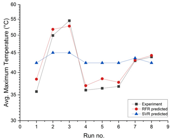
Figure 8.
Comparison of experimental and predicted temperature values for two machine learning models.
4. Conclusions
This experimental study used machine learning models to predict temperature rises during bone drilling. Tests were conducted on bovine femur bone with different drilling settings to develop predictive algorithms. The study examined how various drilling parameters affected the temperature increases throughout the process, leading to several significant findings.
- The RSM method found that the best operating conditions were achieved with a tool diameter of 2 mm, a feed rate of 40 mm/min, and a spindle speed of 1000 rpm.
- This study found that the RFR model outperformed the SVM regression model and RSM, as evidenced by the lower errors in the performance metrics when comparing the three methods.
- The precision in predicting the bone drilling temperatures using the RSM method is 79%, while it is 97.3% with RFR and 25.7% with SVR models.
- The machine learning RFR model enhanced the drilling efficiency and reduced the risk of bone thermal damage by accurately predicting the temperature rises.
4.1. Significance of the Study
This study holds significant theoretical and practical importance for the machining of bone and bone-like materials. It enhances the drilling techniques, leading to more efficient and effective drilling operations by determining the optimal drilling parameters for drilling surgeries. The research highlights the impressive capabilities of machine learning techniques, particularly the RF model, in accurately predicting and optimizing the drilling temperatures. This success suggests a promising future for AI-driven solutions in industrial settings. It encourages the further exploration of machine learning’s potential to enhance the precision and efficiency across various industries. The broader implications of this study extend beyond its specific findings, influencing manufacturing processes, sustainability efforts, and the scope of machine learning in industrial optimization. The insights gained from this research can lead to improved practices and significant advancements, benefiting researchers, companies, and society as a whole.
4.2. Limitations
This study has inherent limitations that need to be acknowledged. The complexity and difficulty of the experimental process resulted in a somewhat limited dataset for the training of the machine learning models. This restriction could impact the accuracy of the predicted temperature values, as models trained on smaller datasets may not perform as well. Additionally, if this research is extended to in vivo real-time medical surgeries, monitoring temperature variations at the drill site presents another challenge. The potential technical solutions include the use of more advanced sensor technologies like real-time temperature sensors placed in the drill bit and the development of new monitoring methods to overcome the identified limitations. The limited duration of surgery and the constraints in using thermocouples for temperature measurement add to the difficulty.
Author Contributions
Conceptualization, M.A.I.; methodology, M.A.I.; software, M.A.I. and A.N.A.; validation, M.A.I., N.S.B.K., R.D., H.T. and M.F.I.; formal analysis, M.A.I.; investigation, M.A.I., N.S.B.K. and K.S.B.; resources, N.S.B.K., M.F.I., K.S.B. and R.D.; data curation, M.A.I.; writing—original draft preparation, M.A.I.; writing—review and editing, M.A.I. and N.S.B.K.; visualization, M.A.I.; supervision, N.S.B.K. and R.D.; project administration, M.A.I. and N.S.B.K.; funding acquisition, M.F.I. and K.S.B. All authors have read and agreed to the published version of the manuscript.
Funding
The authors extend their appreciation to the Researchers Supporting Project number (RSPD2024R1072), King Saud University, Riyadh, Saudi Arabia.
Institutional Review Board Statement
Not applicable.
Informed Consent Statement
Not applicable.
Data Availability Statement
The corresponding author can provide the data used in this study upon request. The data are not publicly available due to a lack of available repositories.
Acknowledgments
The authors extend their appreciation to the Researchers Supporting Project number (RSPD2024R1072), King Saud University, Riyadh, Saudi Arabia.
Conflicts of Interest
The authors declare no conflicts of interest.
References
- Pupulin, F.; Oresta, G.; Sunar, T.; Parenti, P. On the thermal impact during drilling operations in guided dental surgery: An experimental and numerical investigation. J. Mech. Behav. Biomed. Mater. 2024, 150, 106327. [Google Scholar] [CrossRef] [PubMed]
- Mediouni, M.; Kucklick, T.; Poncet, S.; Madiouni, R.; Abouaomar, A.; Madry, H.; Cucchiarini, M.; Chopko, B.; Vaughan, N.; Arora, M.; et al. An overview of thermal necrosis: Present and future. Curr. Med. Res. Opin. 2019, 35, 1555–1562. [Google Scholar] [CrossRef] [PubMed]
- Akhbar, M.F.A.; Yusoff, A.R. Fast & Injurious: Reducing thermal osteonecrosis regions in the drilling of human bone with multi-objective optimization. Measurement 2020, 152, 107385. [Google Scholar]
- Donos, N.; Akcali, A.; Padhye, N.; Sculean, A.; Calciolari, E. Bone regeneration in implant dentistry: Which are the factors affecting the clinical outcome? Periodontology 2000 2023, 93, 26–55. [Google Scholar] [CrossRef] [PubMed]
- Wildemann, B.; Ignatius, A.; Leung, F.; Taitsman, L.A.; Smith, R.M.; Pesántez, R.; Stoddart, M.J.; Richards, R.G.; Jupiter, J.B. Non-union bone fractures. Nat. Rev. Dis. Primers 2021, 7, 57. [Google Scholar] [CrossRef]
- Augustin, G.; Davila, S.; Mihoci, K.; Udiljak, T.; Vedrina, D.S.; Antabak, A. Thermal osteonecrosis and bone drilling parameters revisited. Arch. Orthop. Trauma Surg. 2008, 128, 71–77. [Google Scholar] [CrossRef]
- Islam, M.A.; Kamarrudin, N.S.; Daud, R.; Ibrahim, I.; Razlan, Z.M.; Rani, M.F.H. Drill Bit Design and Its Effect on Temperature Distribution and Osteonecrosis During Implant Site Preparation: An Experimental Approach. J. Phys. Conf. Ser. 2023, 2643, 012020. [Google Scholar] [CrossRef]
- Kung, P.C.; Heydari, M.; Tsou, N.T.; Tai, B.L. A neural network framework for immediate temperature prediction of surgical hand-held drilling. Comput. Methods Programs Biomed. 2023, 235, 107524. [Google Scholar] [CrossRef]
- Agarwal, R.; Singh, J.; Gupta, V. Prediction of temperature elevation in rotary ultrasonic bone drilling using machine learning models: An in-vitro experimental study. Med. Eng. Phys. 2022, 110, 103869. [Google Scholar] [CrossRef]
- Staroveski, T.; Brezak, D.; Udiljak, T. Drill wear monitoring in cortical bone drilling. Med. Eng. Phys. 2015, 37, 560–566. [Google Scholar] [CrossRef]
- Ghavami, P. Big Data Analytics Methods: Analytics Techniques in Data Mining, Deep Learning and Natural Language Processing; Walter de Gruyter GmbH & Co. KG: Berlin, Germany, 2019. [Google Scholar]
- Pandey, R.K.; Panda, S.S. Optimization of bone drilling using Taguchi methodology coupled with fuzzy based desirability function approach. J. Intell. Manuf. 2015, 26, 1121–1129. [Google Scholar] [CrossRef]
- Akgundogdu, A.; Jennane, R.; Aufort, G.; Benhamou, C.L.; Ucan, O.N. 3D image analysis and artificial intelligence for bone disease classification. J. Med. Syst. 2010, 34, 815–828. [Google Scholar] [CrossRef] [PubMed]
- Lu, C.H.; Ko, E.W.C.; Liu, L. Improving the video imaging prediction of postsurgical facial profiles with an artificial neural network. J. Dent. Sci. 2009, 4, 118–129. [Google Scholar] [CrossRef][Green Version]
- Agarwal, R.; Singh, J.; Gupta, V. Predicting the compressive strength of additively manufactured PLA-based orthopedic bone screws: A machine learning framework. Polym. Compos. 2022, 43, 5663–5674. [Google Scholar] [CrossRef]
- Agarwal, R.; Singh, J.; Gupta, V. An intelligent approach to predict thermal injuries during orthopaedic bone drilling using machine learning. J. Braz. Soc. Mech. Sci. Eng. 2022, 44, 320. [Google Scholar] [CrossRef]
- Torun, Y.; Öztürk, A. A new breakthrough detection method for bone drilling in robotic orthopedic surgery with closed-loop control approach. Ann. Biomed. Eng. 2020, 48, 1218–1229. [Google Scholar] [CrossRef]
- Au, E.H.; Francis, A.; Bernier-Jean, A.; Teixeira-Pinto, A. Prediction modeling—Part 1: Regression modeling. Kidney Int. 2020, 97, 877–884. [Google Scholar] [CrossRef]
- Islam, M.A.; Kamarrudin, N.S.; Daud, R.; Ibrahim, I.; Bakar, S.A.; Noor, S.N.F.M. Quantifying the Impact of Drilling Parameters on Temperature Elevation within Bone during the Process of Implant Site Preparation. J. Adv. Res. Appl. Mech. 2024, 116, 1–12. [Google Scholar] [CrossRef]
- Islam, M.A.; Kamarrudin, N.S.; Suhaimi, M.F.F.; Daud, R.; Ibrahim, I.; Mat, F. Parametric Investigation on Different Bone Densities to Avoid Thermal Necrosis during Bone Drilling Process. J. Phys. Conf. Ser. 2021, 2051, 012033. [Google Scholar] [CrossRef]
- Akhbar, M.F.A.; Yusoff, A.R. Multi-objective optimization of surgical drill bit to minimize thermal damage in bone-drilling. Appl. Therm. Eng. 2019, 157, 113594. [Google Scholar] [CrossRef]
- Ali Akhbar, M.F.; Yusoff, A.R. Drilling of bone: Effect of drill bit geometries on thermal osteonecrosis risk regions. Proc. Inst. Mech. Eng. Part H J. Eng. Med. 2019, 233, 207–218. [Google Scholar]
- Shakouri, E.; Haghighi Hassanalideh, H.; Gholampour, S. Experimental investigation of temperature rise in bone drilling with cooling: A comparison between modes of without cooling, internal gas cooling, and external liquid cooling. Proc. Inst. Mech. Eng. Part H J. Eng. Med. 2018, 232, 45–53. [Google Scholar] [CrossRef] [PubMed]
- Hillery, M.T.; Shuaib, I. Temperature effects in the drilling of human and bovine bone. J. Mater. Process. Technol. 1999, 92, 302–308. [Google Scholar] [CrossRef]
- Sui, J.; Sugita, N. Experimental study of thrust force and torque for drilling cortical bone. Ann. Biomed. Eng. 2019, 47, 802–812. [Google Scholar] [CrossRef]
- Islam, M.A.; Kamarrudin, N.S.; Daud, R.; Mohd Noor, S.N.F.; Azmi, A.I.; Razlan, Z.M. A review of surgical bone drilling and drill bit heat generation for implantation. Metals 2022, 12, 1900. [Google Scholar] [CrossRef]
- Li, S.; Shu, L.; Kizaki, T.; Bai, W.; Terashima, M.; Sugita, N. Cortical bone drilling: A time series experimental analysis of thermal characteristics. J. Manuf. Process. 2021, 64, 606–619. [Google Scholar] [CrossRef]
- Wang, Y.; Cao, M.; Zhao, Y.; Zhou, G.; Liu, W.; Li, D. Experimental investigations on microcracks in vibrational and conventional drilling of cortical bone. J. Nanomater. 2013, 2013, 845205. [Google Scholar] [CrossRef]
- Pandithevan, P.; Pandy, N.V.M. Multi-objective optimization for surgical drilling of human femurs: A methodology for better pull-out strength of fixation using taguchi method based on membership function. J. Mech. Med. Biol. 2020, 20, 1950072. [Google Scholar] [CrossRef]
- Pandithevan, P.; Pandy, N.V.M.; Palanivel, C. Development of in-situ temperature prediction models from cadaveric human femur for bone drilling. J. Mech. Med. Biol. 2018, 18, 1850026. [Google Scholar] [CrossRef]
- Moghaddas, M.A. Modeling and optimization of thrust force, torque, and surface roughness in ultrasonic-assisted drilling using surface response methodology. Int. J. Adv. Manuf. Technol. 2021, 112, 2909–2923. [Google Scholar] [CrossRef]
- Akhbar, M.F.A.; Yusoff, A.R. Optimization of drilling parameters for thermal bone necrosis prevention. Technol. Health Care 2018, 26, 621–635. [Google Scholar] [CrossRef] [PubMed]
- Mondal, N.; Mandal, M.C.; Dey, B.; Das, S. Genetic algorithm-based drilling burr minimization using adaptive neuro-fuzzy inference system and support vector regression. Proc. Inst. Mech. Eng. Part B J. Eng. Manuf. 2020, 234, 956–968. [Google Scholar] [CrossRef]
- Song, Z.; Zhao, Y.; Liu, G.; Gao, Y.; Zhang, X.; Cao, C.; Dai, D.; Deng, Y. Surface roughness prediction and process parameter optimization of Ti-6Al-4 V by magnetic abrasive finishing. Int. J. Adv. Manuf. Technol. 2022, 122, 219–233. [Google Scholar] [CrossRef]
- Li, L.-N.; Liu, X.-F.; Yang, F.; Xu, W.-M.; Wang, J.-Y.; Shu, R. A review of artificial neural network based chemometrics applied in laser-induced breakdown spectroscopy analysis. Spectrochim. Acta Part B At. Spectrosc. 2021, 180, 106183. [Google Scholar] [CrossRef]
- Ein-Afshar, M.J.; Shahrezaee, M.; Shahrezaee, M.H.; Sharifzadeh, S.R. Biomechanical evaluation of temperature rising and applied force in controlled cortical bone drilling: An animal in vitro study. Arch. Bone Jt. Surg. 2020, 8, 605. [Google Scholar]


Disclaimer/Publisher’s Note: The statements, opinions and data contained in all publications are solely those of the individual author(s) and contributor(s) and not of MDPI and/or the editor(s). MDPI and/or the editor(s) disclaim responsibility for any injury to people or property resulting from any ideas, methods, instructions or products referred to in the content. |
© 2024 by the authors. Licensee MDPI, Basel, Switzerland. This article is an open access article distributed under the terms and conditions of the Creative Commons Attribution (CC BY) license (https://creativecommons.org/licenses/by/4.0/).