Abstract
This work focuses on the three-dimensional integrated guidance and control (IGC) problem for a flight vehicle with a body-aligned strapdown seeker. The strapdown seeker cannot provide the line-of-sight (LOS) angular rate information and causes difficulties in the controller design. Additionally, external disturbance and gain–loss actuator faults also lead to the loss of control performance. To solve these problems, an extended state observer (ESO) is firstly developed to estimate the LOS angular rate by applying the observed body-line-of-sight angles provided by the body-aligned strapdown seeker. Based on backstepping and dynamic surface control techniques, the fault-tolerant IGC is then designed to deal with the gain–loss actuator fault, and adaptive approaches are applied to improve the robustness of the system. Finally, the uniformly ultimately bounded stability of the flight control system is guaranteed via Lyapunov synthesis, and numerical simulations are conducted to verify the effectiveness of the system.
1. Introduction
Traditionally, the guidance and autopilot design of the flight vehicle are treated as two independent processes, in which the guidance loop is the outer loop to generate the acceleration commands. The autopilot is the inner loop to track the acceleration commands. This method ignores the coupling characteristics of the guidance and autopilot, and requires that the guidance loop has a much slower response speed than autopilot, i.e., the spectral separation rule [1]. However, with the flight envelope becoming larger or the vehicle-target distance becoming smaller, the response speed of the guidance loop may increase, which may further break the spectral separation rule between guidance and autopilot loops and eventually lead to a large miss distance.
In recent years, integrated guidance and control (IGC) has attracted growing research interest for flight vehicles [2] and has been successfully applied in some flight vehicles [3]. IGC treats the guidance and control loops as a whole system and generates the fin deflection command directly [4]. From the perspective of control theory, the relative motion of the flight vehicle and the target, and the attitude model of the flight vehicle are combined, in the framework of IGC. The motion model of the flight vehicle can be regarded as a high-order uncertain nonlinear dynamical system containing matched and unmatched disturbances [5]. Furthermore, due to the harsh flight environment, some parameters, such as aerodynamical parameters, are not easy to obtain accurately, which may introduce parameter perturbation. Apart from the disturbance and parameter perturbation, gain–loss actuator faults are another significant factor, which may influence the stability of the system.
To some extent, actuator faults can be seen as a special disturbance for the flight vehicle system, which, however, is input-related. The upper bound of the parameter perturbation or disturbance item can usually be parameterized by a known or unknown constant and a known function. In contrast, if taking the actuator fault into consideration, the uncertain item can no longer be parameterized before the control law is determined. Therefore, fault-tolerant IGC (FTIGC) requires further research.
As mentioned earlier, the flight vehicle model can be treated as a high-order nonlinear system with the states describing the relative motion of the flight vehicle and target and the attitude motion of the flight vehicle. According to the parallel approaching method, it is expected that the line-of-sight (LOS) angular rate should converge to zero. To achieve the control target, all the state information should be measured or calculated. The seekers, including the gimbaled seeker and strapdown seeker, are devices used to provide the relative motion information. Compared with the gimbaled seeker, the strapdown seeker removes the mechanical servo system, which decreases the cost and the complexity of the structure, and increases the reliability [6]. Instead, the strapdown seeker is body-aligned. Hence, the optical axis of the seeker will not point to the target and only the body-line-of-sight (BLOS) angles can be provided [7,8]. The absence of the LOS angular rate will indeed pose a significant challenge in the design of guidance laws.
According to the discussion above, this paper focuses on the problem of IGC considering the potential gain–loss actuator fault, without the LOS angular rate measurement information. To achieve this, the LOS angular rate is reconstructed by an Extend State Observer (ESO) with the measured BLOS angle information. Furthermore, backstepping-based FTIGC is then investigated with the estimated LOS angular rate.
The main contributions of this work are as follows:
- (1)
- A linear ESO is established based on the measured body-LOS angle information, and the uniformly ultimately bounded stability of the estimation error of the LOS angular rate is guaranteed.
- (2)
- Based on the backstepping technique and the proposed ESO, the FTIGC scheme is developed to obtain control inputs without separated guidance and command systems design, and the computational explosion problem is avoided via dynamic surface design.
- (3)
- Adaptive control laws are designed to deal with the lumped uncertainties consisting of the gain–loss actuator fault, external disturbances, and aerodynamic perturbation, which significantly enhances the robustness of the flight control system.
The rest of this work is organized as follows. Section 2 shows some related works about IGC and the LOS angular rate extraction. Section 3 presents the modeling and the problem formulation, and Section 4 lays down the design of the fault-tolerant integrated guidance and control scheme. Numerical simulations are carried out in Section 5 and conclusions are given in Section 6.
2. Related Works
2.1. IGC
Compared with the traditional guidance and control system design, IGC treats the guidance system and control system as a whole system, which eliminates the assumption that the guidance system has a faster response speed than the control system. Therefore, it solves the coordination problem of the spectral characteristics of guidance and control systems. This section presents a brief introduction to IGC.
IGC considers the attitude dynamics in the guidance subsystem design and produces the fin deflection commands directly. In early years, channel-separated IGC was widely researched, in which the Six-Degrees-of-Freedom (6DOF) motion of the flight vehicle is decomposed into longitudinal and lateral motion planes, and IGC is designed independently for each plane. This method reduces the order of the system and the complexity of the control parameter tuning. However, essentially, the spatial motion of the flight vehicle is located in SE(3) space. Hence, the above-mentioned decomposition method does not consider the coupling of the longitudinal and lateral motion planes, which may reduce the system precision. To simplify the problem, in [2], IGC was treated as a linear optimal control problem by ignoring nonlinear items. To consider the nonlinearities, State-Dependent Riccati Equation (SDRE)-based IGC was proposed [9]. In SDRE-based IGC, the 6DOF motion of the flight vehicle was rewritten as a pseudo-linear state space equation in which the coefficients are state-dependent. In what follows, by solving an online Riccati Equation (RE), similar to the Linear Quadratic Regulator (LQR) technique, the control input can be obtained. To avoid solving the online RE, the θ-D technique was proposed [10,11]. Apart from this, feedback linearization is also usually applied to obtain a linear IGC model, and based on that, the LQR method can be applied. By comparison, SDRE, θ-D, or feedback linearization-based IGC has weak robustness against uncertainties because the accurate information of the model is required. To improve the robust of the system, an adaptive IGC for pitch channel was designed with a so-called Nussbaum function being applied to deal with the disturbance [12].
In order to improve the performance of the flight vehicle system, in recent years, three-dimensional IGC was proposed, which combines the nonlinear flight vehicle models with the vehicle-object pursuit model in three-dimensional space. Three-dimensional IGC fully describes the 6DOF motion of the flight vehicle, and channel-separated IGC is a simplification of the three-dimensional IGC by assuming that the angle between the LOS and missile velocity is small or almost constant [13]. Several nonlinear control methods are employed, such as sliding mode control (SMC) [14], the small-gain theorem [15], the backstepping approach [16], and intelligent control [17]. With the backstepping approach, the high-order nonlinear system of the flight vehicle is divided into multiple subsystems with the cascade structure. For each subsystem, SMC, adaptive control, and intelligent control can be applied for command tracking and disturbance rejection. The small-gain theorem-based IGC treats the system of the flight vehicle as an interconnected system, combined with the guidance subsystem and control subsystem. The guidance law and control law are designed separately such that each subsystem is input-to-state-output practically stable with its input and the output of another subsystem [15,18].
The above-mentioned forms of IGC assume that the actuator (fin) system can respond to the command of IGC. However, in practice, due to some physical constraints, the flight vehicle may suffer from the actuator fault problem, which may degrade system performance and lead to instability of the system. The fault-tolerant ability of IGC will significantly improve the robustness of the system. To this end, fault-tolerant control (FTC) greatly improves the adaptability to actuator faults, and it falls into two main categories: active FTC and passive FTC. Active FTC usually contains a fault detection and diagnosis (FDD) module [19] and a fault-tolerant controller design module, while passive FTC only contains the latter. In active FTC, faults are detected, isolated, and then estimated by the FDD module [20], which provides real-time information for the systems, and then the control strategy or even the controller is reconstructed. In this way, active FTC can deal with different types of faults effectively, but more sensors and computational capacity are required. Passive FTC needs no real-time information on faults and thus a faster response and simple structure are achieved, but it is usually effective only for known fault types. As the common module of active FTC and passive FTC, a well-designed fault-tolerant controller is important to improve the adaptability to actuator faults. For over-actuated systems or systems with redundant actuators, a control allocation-based fault-tolerant controller could significantly improve the reliability of the system. In [21], a closed-loop feedback integral-based allocation controller is proposed for an actuated flight vehicle to track the attitude command. The control moment is allocated to the variable span and sweep of morphing flight vehicles in [22]. For systems without additional power units, maintaining stability is the priority. In this case, actuator faults are always viewed as unpredictable dynamics or uncertainties, and then sliding mode control, adaptive control theories, and intelligent control are implemented to improve the robustness. A sliding mode fault-tolerant controller is designed in [23] to solve the trajectory tracking problem of flight vehicles with actuator faults. To enhance the robustness of aircraft control systems with actuator faults and disturbances, an adaptive fuzzy controller is designed in [24].
The proposed FTIGC combines the three-dimensional IGC and passive FTC techniques to deal with the disturbance and actuator fault.
2.2. LOS Angular Rate Extraction
All the forms of IGC mentioned above require accurate information about the relative motion between the flight vehicle and the object. As for the strapdown seeker, since the detector of the strapdown seeker is fixed with the body of the flight vehicle, the directly measured information is the BLOS angles instead of the LOS angles. For example, as is shown in Figure 1, if only the longitudinal motion is considered, the measured information for the gimbaled seeker is qz and its time derivative . As for the strapdown seeker, the measured information is the BLOS angle . Assume that is the pitch angle of the flight vehicle; it has and , where is the pitch angular rate. Therefore, the unmeasured indicates that cannot be obtained or calculated directly. Therefore, it is useful to discuss the LOS angular rate extraction problem for flight vehicles with a strapdown seeker.
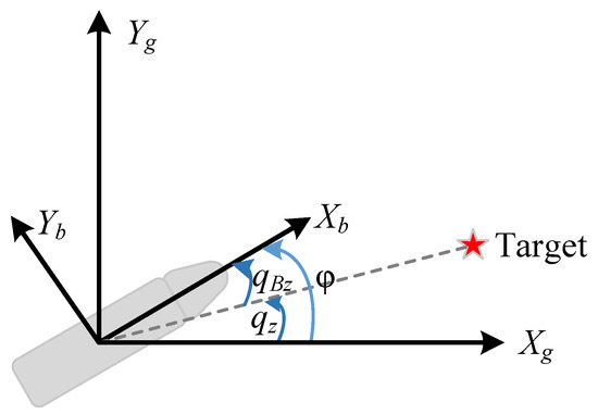
Figure 1.
Diagram of the gimbaled seeker and strapdown seeker in the longitudinal plane.
A straightforward approach involves numerically differentiating the measured BLOS angles to obtain the BLOS angular rate, which, however, may amplify the measurement noise. A Kalman Filter (KF) is proposed for the INS/seeker [25] and its observability problem was analyzed. As a promotion, the Extended Kalman Filter (EKF) [26] and Unscented Kalman Filter (UKF) [7] are also applied to extract the LOS angular rate. The reconstruction of the LOS angular rate is researched in [7], by combing the Tracking Differentiator and UKF. The Extended State Observer (ESO) has excellent performance in estimating the states and disturbance, and is expanded to IGC. The IGC strategy of the missile with a strapdown seeker is researched in [27], which, however, only considers the longitudinal-plane movement.
These mentioned references only discuss how to extract the LOS angular rate from the measured BLOS angles; however, the influence of the estimated LOS angular rate on the system has not been discussed.
3. Preliminaries
In this section, the Six-DOF dynamical model of the flight vehicle is first established. In what follows, the relative motion of the flight vehicle with a strapdown seeker in 3D space is given. The control objectives are also demonstrated. First of all, we define that denotes the Euclidean norm of the vector . For a given vector , represents its cross-product matrix, which can be given by
Apparently, always holds for any vectors . En denotes the n-dimensional identity matrix.
3.1. Model Derivation
The force diagram of the flight vehicle is illustrated in Figure 2, in which is the body coordinate system. V is the velocity of the flight vehicle.
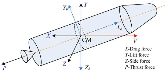
Figure 2.
Force diagram of the flight vehicle.
The nonlinear attitude dynamics of the flight vehicle with uncertainties can be described by [28]
where are the bank angle, angle of attack, and angle of sideslip, respectively. Y and Z are the lift and side forces. m is the mass of the flight vehicle and g is the gravity acceleration value. θ is the flight path angle and is the angular rate vector. V is the velocity value of the flight vehicle. is the inertia matrix of the flight vehicle and is the aerodynamic moment, which will be given later. denotes the uncertainties. Furthermore, the translational dynamics can be given by
where x, y, z are the positions of the flight vehicle. is the flight heading angle. X is the drag force and P is the thrust force. In our research, only the terminal guidance phase is considered. Therefore, P = 0 is assumed.
The lift and side force, Y and Z, are given by
in which is the dynamic pressure and ρ is the air density. S is the reference size. and are partial derivatives of the lift force coefficient with respect to α and the side force coefficient to β, respectively. dY and dZ are the uncertainty terms caused by modeling errors and neglecting higher-order terms in approximation. Similarly, the aerodynamic moment can be simplified as
where L represents the reference length. and denote the three axis fin deflections, respectively. represents the partial derivatives of the three axis moment coefficients with respect to α, β, or fin deflections . , , and are the uncertainty terms of the aerodynamic moment.
3.2. Relative Motion of the Flight Vehicle with a Moving Object
Firstly, as shown in Figure 3, we denote the inertial coordinate system by , the body coordinate system by , the LOS coordinate system by , and the body-LOS coordinate system by . Moreover, the ballistic and velocity coordinate systems are denoted by and respectively. The orientations between these coordinate systems are illustrated in Figure 4, showing the definition of the Euler angles, angle of attack, angle of sideslip, angle of bank, LOS angles, and body-LOS angles [29].
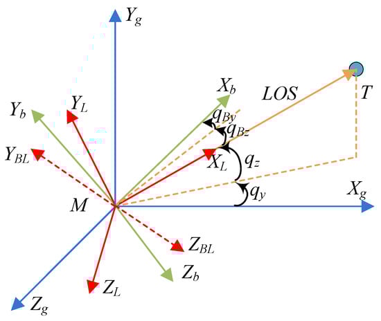
Figure 3.
Three-dimensional geometry of the flight vehicle and the object.
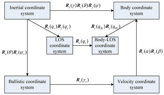
Figure 4.
The transformation of the coordinate systems.
The three-dimensional vehicle-object pursuit model can be described by the following nonlinear differential equation [8,30]:
where R is relative distance. qz and qy are the elevation and azimuth angles of the LOS and their time derivatives, and and are the LOS angular rates. and represent the acceleration vectors of the object and the flight vehicle, expressed in the LOS frame.
According to the parallel approaching method [31], keeping the LOS direction ultimately constant, i.e., , is one of the sufficient conditions to acquire an interception of the object [13]. In addition, the relative distance R is usually uncontrollable in the terminal guidance phase. Thus, the last two equations of (5) can be rearranged as
As for the flight vehicle, its acceleration in the LOS frame can be given by
where is the rotation matrix from the velocity frame to the LOS frame, while is that from the inertial frame to the LOS frame. Supposing that the Skid-to-Turn (STT) maneuver is adopted to improve the performance, the angle of bank, , is expected to approximate zero. Thus, by combining (3) and (7), through simple calculations, it can be seen that
where is the rotation matrix from the ballistic frame to the LOS frame.
3.3. Strapdown Seeker Model
The strapdown seeker does not have a physical platform to achieve object tracking. As a result, it cannot provide the measurement information with respect to the inertial frame, such as LOS angles ( and ) and their time derivatives. Instead, it can only provide the body-LOS angles, and , as defined in Figure 3.
Body-LOS angles, and , describe the reorientation between the body-LOS frame and the body frame. Without loss of generality, it is assumed that the optical axis of the strapdown seeker is aligned along the x-axis of the body frame. With the definition of and , the optical axis can be described in the body frame as [8,30]
Similarly, in the inertial frame, the vector of the LOS can also be given as
Therefore, with the help of the relationship that , this gives
where is the rotation matrix of the inertial frame with respect to the body reference frame, which can be calculated by Euler angles obtained from the navigation system.
3.4. Fault-Tolerant Integrated Guidance and Control Problem Formulation
The actuator fault may cause significant results, and even the failure of the task. The actuator fault in this paper is described as [32]
where is the fin deflection command and is the actual actuator output. is the fin healthy factor matrix indicating the efficiency of the fins. Apparently, always holds. denotes the complete failure, i.e., this fin cannot work completely. indicates that no fault occurs in this fin.
Let , , . Then, according to Section 3.1 and Section 3.2, the integrated guidance and control model of the flight vehicle can be summarized as
where .
Before demonstrating the IGC design, the following assumptions are proposed.
Assumption 1.
Ref. [24] the complete failure of the fin is not taken into consideration. It is assumed that . Moreover, is assumed to be unknown. Furthermore, there is an unknown constant such that .
Assumption 2.
Ref. [23] the external disturbance di (i = 1, 2, 3) in (13) is assumed to be unknown but bounded. That is to say, there exists an unknown positive constant satisfying that .
Assumption 3.
Ref. [33] The control gain matrices, , (i = 1, 2, 3), are all bounded and invertible.
The control objective can be summarized as designing an IGC law for the flight vehicle with a potential actuator fault to intercept a moving object with strong robustness when the LOS angular rates are not available. According to the parallel approaching method, it is expected that the LOS angular rate vector .
4. FTIGC Design-Based LOS Angular Rate and the Target Motion Estimation Information
In this section, the LOS angular rate and the target acceleration are firstly estimated with the application of the Extended State Observer (ESO) based on the measured body-LOS angle information. In what follows, an FTIGC law is proposed in which the DSC technique is used to avoid the problem of explosion of the differential. The control structure diagram is described in Figure 5.
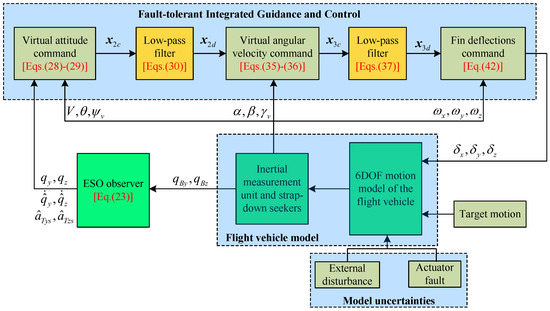
Figure 5.
Control structure diagram of the flight vehicle with a strapdown seeker.
4.1. LOS Angular Rate Reconfiguration and Target Acceleration Estimation
As mentioned previously, the strapdown seeker can only provide the body-LOS angles, and . According to (11), it has
That is to say, the body-LOS angles will uniquely determine the LOS angles. Although direct differentiation of qz and qy can obtain the LOS angular rates, it may magnify the measurement noise. Therefore, the ESO technique is applied. Letting , and , (6) will furthermore yield
in which and are given as
Remark 1.
The body-aligned accelerometer can measure the apparent acceleration in the body reference frame while the gravity acceleration in the inertia frame can also be calculated. With the measured body-LOS angles and calculated LOS angles, can be obtained easily.
In what follows, a linear ESO is designed as [34]
where , , and are the diagonal observer gains to be designed. The observing errors are designed as and . Considering (21)–(23), this gives
Note that (24) can be rewritten as
Apparently, if the selection of the observer gains, , , and , makes the matrix
be Hurtwiz, the observer errors will be Uniform Ultimate Boundedness (UUB), as long as . That is to say, there exists a small positive constant satisfying . As a result, it can be concluded that the states of the ESO will converge to the LOS angles, LOS angular rates, and target acceleration, i.e., .
Assuming that , through simple calculation, the characteristic polynomial of can be given by
Therefore, the selection of the observer gain matrices will determine the bandwidth frequency of the observer. If the desired bandwidth frequency of the observer is , the observer gains can be given by
Note that a larger will result in a faster convergence rate, which, however, may enlarge the observer noise. Thus, the observer gains can be determined by selecting a proper bandwidth frequency.
4.2. FTIGC Design
In the previous subsection, the LOS angular rates, and , can be estimated by the ESO, and the attitude vector and angular velocity can be measured. Thus, the full states of (13) are available. Furthermore, the ESO can also provide the estimated target acceleration components, and . In what follows, the FTIGC technique is developed.
Recall that (13) is a cascade dynamic system with a matched or unmatched disturbance. The control procedure includes three steps, motivated by the backstepping techniques.
- Step 1, Virtual attitude command design
With the reconfigured target accelerations , and estimated LOS angular rates , promoting as the virtual control input, design as
where is the estimated vector with the ESO’s outputs, and , replacing and , substituting in (14). is the positive gain matrix. represents the adaptive parameters, updated by
where is the positive gain. To the avoid explosion of differential, a low-pass filter is designed, motivated by the DSC technique [1], as
where denotes the filter time constant and is the state of the filter. Letting and , and substituting (28) into (13) will yield
in which . The upper bound of has been analyzed in Section 4.1, which will further yield the boundness of . Therefore, as stated earlier, it can be implied that there must exist an unknown positive constant satisfying . Additionally, to analyze the stability of the subsystem, a Lyapunov function candidate is selected as
whose time derivatives can be given by
As a result, if the boundary layer error converges to a zero vector, i.e., , it has . According to the Lyapunov theorem and invariant set lemma, the asymptotical stability of this subsystem can be concluded.
- Step 2, Virtual angular velocity command design
The STT maneuver is adopted and the command bank angle is set to be zero. Treating as the virtual control input of the second dynamical equation of (13), this step aims to design a virtual angular velocity command to drive to converge to . Defining and , it will come to
where can be calculated through (30). Following the steps of the backstepping techniques, the virtual control input, , is designed as
where . is the positive-definite gain matrix and is the estimate value of , provided by the following adaptive law:
where λ2 is the positive real number. Similarly, a low-pass filter
is adopted.
Define and , and select a Lyapunov function as
The time derivative of V2 can be directly given, considering (30), (33)–(36), by
where Young’s inequality is applied and μ1 is an arbitrary constant which only helps to proceed with the analysis. If the boundary layer error, and , can be ignored, and as long as is satisfied, it will eventually yield
where . Define the following compact set as
and it can be analyzed that the system trajectories will eventually converge to the compact subset defined by , which contains the origin and can be set to an arbitrarily small size by selecting the appropriate control parameters. Therefore, according to the discussion above, we can conclude that .
- Step 3, Fin deflection command
In this step, a control law is designed for fin deflections δ with fault tolerance ability to track the virtual angular velocity command , provided by the low-pass filter (37). With the definition of , and considering the potential actuator fault (12), the dynamics of the tracking error can be given by
The control law is designed as
where and c3 is a constant to be defined later. To analyze the stability of the system, the Lyapunov function candidate here is selected as
Note there exist constants satisfying
where and the following equation:
can be derived. Therefore, the time derivative of V3 is
Substituting the control law (42) into (46) will further yield
where μ2 is an arbitrary constant. If is satisfied, the following compact set is defined by
which can be small enough by selecting proper control parameters. Thus, it can be concluded that the LOS angular rates and tracking errors are also UUB, and then the control target can be achieved.
Remark 2.
The low-pass filters in (30) and (37) both have extra items and , compared with the low-pass filters described in [35,36]. These extra items help to eliminate the influence of the boundary layer errors caused by the low-pass filter. For example, as in (39), the item may break the stability of the system. To avoid this, the item in (37) will counteract the same item in (39).
5. Simulation
In this section, the effectiveness of the proposed FTIGC for the flight vehicle with a strapdown seeker is verified by numerical simulations. The full aerodynamic forces and moments in the simulation are given by [33]
where is the zero-lift drag coefficient. , , , , and are the partial derivatives of the drag force coefficient with respect to α, β, , , and . is the second partial derivative of the drag force coefficient with respect to α and β. , , and are the partial derivatives of the lift force coefficient with respect to α, β, and . , , and are the partial derivatives of the side force coefficient with respect to α, β, and . Similarly, , , and are the partial derivatives of the rolling moment coefficient with respect to α, β, and ; and are the partial derivatives of the yawing moment coefficient with respect to β and ; and and are the partial derivatives of the pitching moment coefficient with respect to α and .
Considering the physical limitations, each fin deflection should be constrained to ±20°. Apart from this, the nominal values of the parameters related to the flight vehicle are listed in Table 1.

Table 1.
The nominal values of the flight vehicle-related parameters.
The flight vehicle initially locates at in the Inertial reference frame and the initial values of the roll, yaw, and pitch angles are set to be , , and . The initial velocity, flight path angle, and heading angle of the flight vehicle are assumed as , , and . The initial angular rate vector is .
The control parameters are selected as follows: , , , , , , , , . The simulation includes three cases with the same control parameters but different actuator fault models for fixed or moving objects.
- Case1. No actuator fault happens. In other words, .
- Case2. The actuator healthy factors are all constants, which are set as , and .
- Case3. The actuator healthy factors are not constants, which are set aswhere refers to the random function distributed on the open interval (−1, 1).
Furthermore, to verify the robustness of the proposed FTIGC, the parameter perturbations are also considered in the simulation. Letting represent certain nominal parameters given in Table 1, the actual values p are designed as .
Remark 3.
The observer’s dynamical errors may destroy the performance of the FTIGC, especially in the initial period when the ESO works. To avoid this phenomenon, in our work, it is designed that
in which and represent the starting working times of the FTIGC and ESO, respectively. is set to be 0.8 s in the simulation.
5.1. For a Fixed Object
It is required that the flight vehicle will arrive at a fixed position, located on , in this subsection. The simulation results are given in Figure 6, Figure 7, Figure 8, Figure 9, Figure 10, Figure 11, Figure 12 and Figure 13. From Figure 6 and Figure 7, it can be found that the flight vehicle will eventually fly toward the object in these three cases under the proposed FTIGC. The miss distances for these three cases, as shown in the enlarged figure of Figure 6, are no more than 1 m and the hitting time is about 38 s. According to Figure 8, the body-LOS angles will converge to certain constant values, whereas the values are different for these three cases because the terminal angle constraint is not considered in our manuscript. Figure 9 is the time response of the LOS angular rate. It is indicated that the LOS angular rates will converge to zero, which also verifies the effectiveness of the proposed FTIGC with the help of the parallel approaching principle. Figure 10 shows the time response of the angles of attack and sideslip. It can be found that the angles of attack and sideslip are limited to 5° and 1°, respectively, while their tracking errors have an accuracy of 0.01°, indicating the control law has great tracking performance. Figure 12 shows the time response of the angular velocity and its tracking error, which has the accuracy of 0.01°/s. Figure 10 and Figure 12 simultaneously demonstrate that the inner loop has good tracking performance on the virtual command from the outer loop with the application of the DSC. Figure 13 reports that the fin deflections will not touch the saturation limit. Therefore, it can be concluded that the proposed FTIGC performs well for the scenario in which the flight vehicle arrives at a fixed object, whether the actuator is healthy or not.
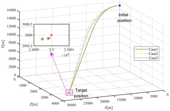
Figure 6.
Trajectories of the flight vehicle and the object.
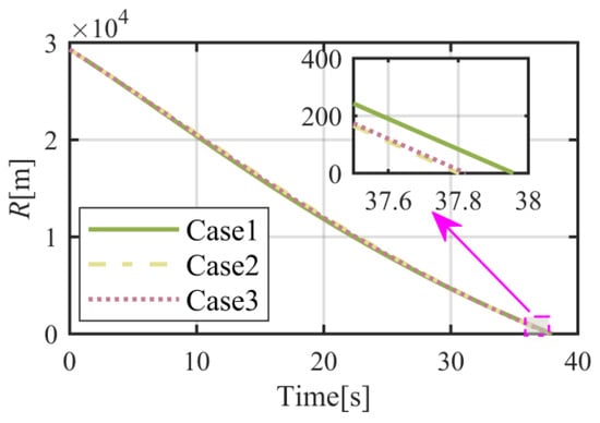
Figure 7.
Time histories of flight vehicle-object relative motion range.
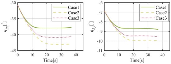
Figure 8.
Time histories of the body-LOS angles.
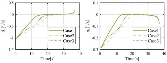
Figure 9.
Time histories of the LOS angular rates.
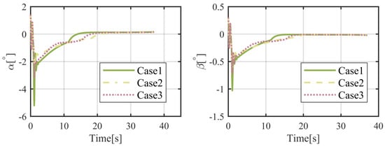
Figure 10.
Time histories of the attack and sideslip angles of the flight vehicle.
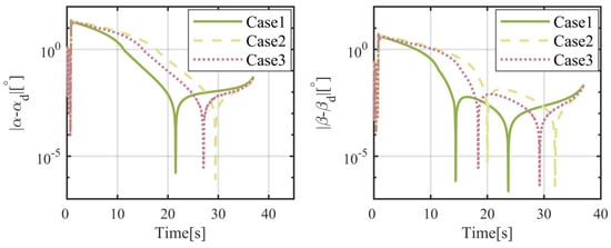
Figure 11.
Time histories of the tracking errors of the attack and sideslip angles.
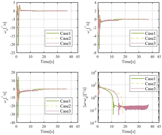
Figure 12.
Time histories of the angular velocities and their tracking errors.
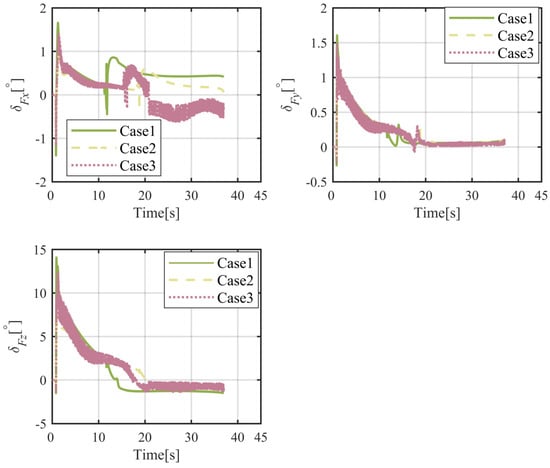
Figure 13.
Time histories of the actual fin deflections.
5.2. For a Moving Object
In this subsection, the simulation is conducted for a moving object under the proposed FTIGC for the three same cases. The motion of the object is described by
where , , and are the position, velocity, and acceleration vectors in the inertial reference frame, respectively, with the initial values of the position, velocity, and the accelerations set as
The results of numerical simulations for moving objects are demonstrated in Figure 14, Figure 15, Figure 16, Figure 17, Figure 18, Figure 19, Figure 20 and Figure 21. As shown in Figure 14, the object can be intercepted in about 40.5 s by the flight vehicle under the proposed FTIGC, whether or not the actuator fault happens. Figure 15 reports the time response of the relative distance, which will converge to zero. Figure 16 shows the time histories of the BLOS angles. It is indicated that the BLOS angles will converge to certain constant values. Figure 17 indicates that LOS angular rates will also converge to zero in these three cases. With the application of the parallel approaching principle, the effectiveness of the proposed FTIGC can be proved. Figure 18 and Figure 19 indicate the time histories of the angles of attack and sideslip, and their tracking errors with respect to the output of the low pass filter (30). It can be found that the tracking accuracy reaches 0.05°. Similarly, Figure 20 shows the three-axis angular velocity and tracking errors with respect to are about 0.01°/s, which partly verifies the effectiveness of the control law. Figure 21 shows the fin deflection responses and it is evident that all the fin deflections will satisfy the saturation constraint. All these results show the proposed FTIGC has good performance for a moving object.
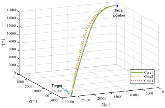
Figure 14.
Trajectories of the flight vehicle and the object.
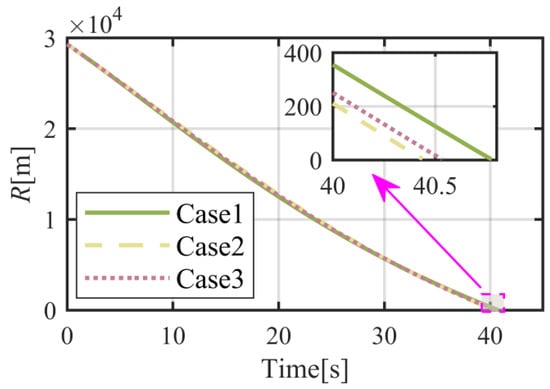
Figure 15.
Time histories of the flight vehicle-object relative motion range.
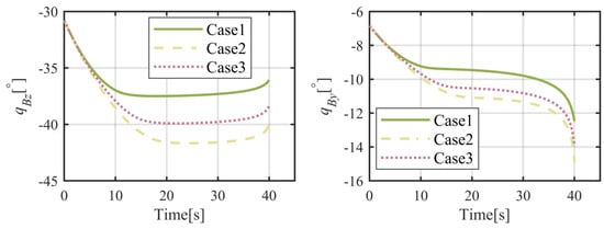
Figure 16.
Time histories of the body-LOS angles.
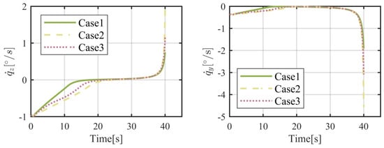
Figure 17.
Time histories of the LOS angular rates.
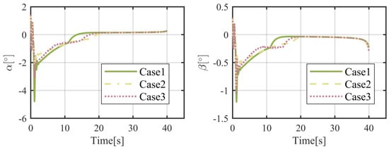
Figure 18.
Time histories of the attack and sideslip angles of the flight vehicle.
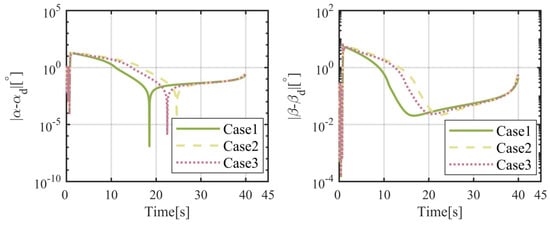
Figure 19.
Time histories of the tracking errors of the attack and sideslip angles.
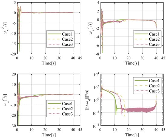
Figure 20.
Time histories of the angular velocities and its tracking errors.
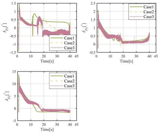
Figure 21.
Time histories of the actual fin deflections.
5.3. Comparison
To show the performance of the proposed IGC, the results are compared with the traditional integrated guidance control law (TIGC) proposed in [28]. In this subsection, similar to Section 5.1, it is expected that the flight vehicle will arrive at a fixed location. It is assumed that the healthy factors are the same and constant for each fin. Three cases are researched, which have different healthy factors, and all other simulation conditions and control parameters are the same as in Section 5.1 for both schemes. The miss distance is used to evaluate the control performance. The simulation results are given in Figure 22 and Figure 23, and Table 2.
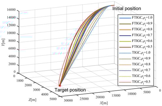
Figure 22.
Trajectories of the flight vehicle for different fin healthy factors under FTIGC and TIGC.
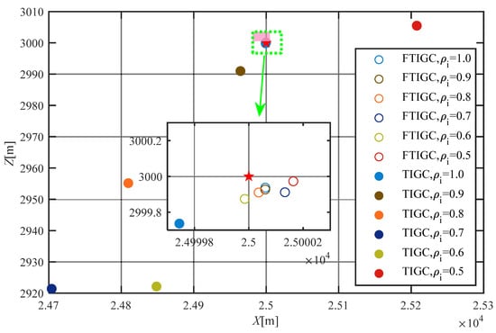
Figure 23.
Landing points of the flight vehicle for different fin healthy factors under FTIGC and TIGC.
Table 2.
Miss distance for different healthy factors under TIGC and FTIGC.
Figure 22 shows the three-dimensional trajectories of the flight vehicle with the application of the proposed FTIGC and TIGC when different fin healthy factors are considered. Figure 23 reports the miss distances for these cases, and the miss distances for these cases are also listed in Table 2. It can be found that the flight vehicle can arrive at the target position accurately (the miss distance is less than 0.5 m), under the TIGC in [28] and the proposed FTIGC, if no actuator fault happens. However, when the fin fault happens, the miss distance for flight vehicle under TIGC will increase rapidly with the fin health factor decreasing. It means that TIGC has weak robustness for an actuator fault. Instead, the flight vehicle under FTIGC has a similar miss distance for different actuator healthy factors. That is to say, it can be concluded that FTIGC will effectively improve the robustness of the parameter perturbation, disturbance, and actuator fault.
In summary, from the discussion in Section 4 and Section 5, it can be found that the proposed FTIGC can help the flight vehicle with a strapdown seeker to accurately fly to a fixed or moving target, even when the fin fault occurs. However, we have to point out that the mechanism by which the control parameters and the healthy factors influence the control performance is still unclear, and practical principles to help us select the control parameters cannot be provided. Further, the semi-physical simulations and experiments of the proposed IGC still need further work.
6. Conclusions
This paper develops an FTIGC for flight vehicles without LOS angle rate measurement information, considering the potential actuator fault. To begin with, the transformation relationship between the LOS angles and BLOS angles is established and an ESO is designed by observing BLOS angles, providing the estimation of the LOS angular rate for feedback and object acceleration information for feedforward. An FTIGC, based on the adaptive backstepping and DSC techniques, subject to the external disturbance and actuator fault, is proposed, such that LOS angular rates will converge to zero. With the application of the parallel approaching principle, it can be concluded that the flight vehicle will accurately arrive at the object position. The effectiveness of the proposed FTIGC and the robustness of the system are verified theoretically and numerically. In our future work, we will pay more attention to analyzing the influence of the control parameters and application in the hardware environment.
Author Contributions
Conceptualization, X.Y. and S.L.; methodology, X.Y.; software, X.Y. and F.Z.; validation, S.L.; formal analysis, X.Y.; investigation, X.Y.; resources, S.L.; data curation, X.Y. and F.Z.; writing—original draft preparation, X.Y. and F.Z.; writing—review and editing, X.Y. and S.L.; visualization, X.Y.; supervision, S.L.; project administration, F.Z.; funding acquisition, F.Z. All authors have read and agreed to the published version of the manuscript.
Funding
This research was supported by the Science and Technology Innovation Program of Hunan Province (2023RC3265).
Institutional Review Board Statement
Not applicable.
Informed Consent Statement
Not applicable.
Data Availability Statement
The raw data supporting the conclusions of this article will be made available by the authors on request.
Conflicts of Interest
Authors Xiaojun Yu and Fuzhen Zhang were employed by the company Hunan Vanguard Group Co., Ltd. The remaining authors declare that the re-search was conducted in the absence of any commercial or financial relationships that could be construed as a potential conflict of interest.
References
- Song, H.; Zhang, T.; Wang, X. Integrated Interceptor Guidance and Autopilot Design via Robust Dynamic Surface Control. In Proceedings of the 2018 IEEE CSAA Guidance, Navigation and Control Conference (CGNCC), Xiamen, China, 10–12 August 2018; pp. 1–6. [Google Scholar] [CrossRef]
- Williams, D.; Richman, J.; Friedland, B. Design of an Integrated Strapdown Guidance and Control System for a Tactical Missile. In Proceedings of the Guidance and Control Conference; American Institute of Aeronautics and Astronautics, Gatlinburg, TN, USA, 15–17 August 1983. [Google Scholar] [CrossRef]
- Sun, J.; Song, S.; Wu, G. Tracking Control of Hypersonic Vehicle Considering Input Constraint. J. Aerosp. Eng. 2017, 30, 04017073. [Google Scholar] [CrossRef]
- Pan, Z.; Wang, W.; Xiong, S.; Lu, K. Three Dimensional Integrated Guidance and Control for Slide to Turn Missile with Input Saturation. In Proceedings of the 2016 Chinese Control and Decision Conference (CCDC), Yinchuan, China, 28–30 May 2016; pp. 2554–2559. [Google Scholar]
- Chang, J.; Guo, Z.; Cieslak, J.; Chen, W. Integrated Guidance and Control Design for the Hypersonic Interceptor Based on Adaptive Incremental Backstepping Technique. Aerosp. Sci. Technol. 2019, 89, 318–332. [Google Scholar] [CrossRef]
- Cho, N.; Kim, Y. Optimality of Augmented Ideal Proportional Navigation for Maneuvering Target Interception. IEEE Trans. Aerosp. Electron. Syst. 2016, 52, 948–954. [Google Scholar] [CrossRef]
- Pei, W.; Ke, Z. Research on Line-of-Sight Rate Extraction of Strapdown Seeker. In Proceedings of the The 33th Chinese Control Conference, Nanjing, China, 28–30 July 2014; pp. 859–863. [Google Scholar]
- Zhang, D.; Song, J.; Zhu, Y.; Jiao, T.; Zhao, L. Integrated Elastic Identification and LOS Angular Rate Extraction for Slender Rockets: A Continuous-Discrete Maximum Correntropy Kalman Filter Approach. Aerosp. Sci. Technol. 2024, 150, 109174. [Google Scholar] [CrossRef]
- Vaddi, S.; Menon, P.; Ohlmeyer, E. Numerical SDRE Approach for Missile Integrated Guidance–Control. In Proceedings of the AIAA Guidance, Navigation and Control Conference and Exhibit, Hilton Head, SC, USA, 20–23 August 2007; American Institute of Aeronautics and Astronautics: Reston, VA, USA, 2007. [Google Scholar] [CrossRef]
- Zhou, D.; Li, Q. Indirect Robust Control of Agile Missile via Theta-D Technique. Def. Technol. 2014, 10, 269–278. [Google Scholar] [CrossRef]
- Xin, M.; Balakrishnan, S.N.; Ohlmeyer, E.J. Integrated Guidance and Control of Missiles with θ-D Method. IEEE Trans. Contr. Syst. Technol. 2006, 14, 981–992. [Google Scholar] [CrossRef]
- Liang, X.; Hou, M.; Duan, G. Adaptive Dynamic Surface Control for Integrated Missile Guidance and Autopilot in the Presence of Input Saturation. J. Aerosp. Eng. 2015, 28, 04014121. [Google Scholar] [CrossRef]
- Wang, W.; Xiong, S.; Wang, S.; Song, S.; Lai, C. Three Dimensional Impact Angle Constrained Integrated Guidance and Control for Missiles with Input Saturation and Actuator Failure. Aerosp. Sci. Technol. 2016, 53, 169–187. [Google Scholar] [CrossRef]
- Lai, C.; Wang, W.; Liu, Z.; Liang, T.; Yan, S. Three-Dimensional Impact Angle Constrained Partial Integrated Guidance and Control With Finite-Time Convergence. IEEE Access 2018, 6, 53833–53853. [Google Scholar] [CrossRef]
- Yan, H.; Ji, H. Integrated Guidance and Control for Dual-Control Missiles Based on Small-Gain Theorem. Automatica 2012, 48, 2686–2692. [Google Scholar] [CrossRef]
- Gao, C.; Jiang, C.; Zhang, Y.; Jing, W. Three-Dimensional Integrated Guidance and Control for Near Space Interceptor Based on Robust Adaptive Backstepping Approach. Int. J. Aerosp. Eng. 2016, 2016, 1–11. [Google Scholar] [CrossRef]
- Zhou, L.; Liu, L.; Cheng, Z.; Wang, B.; Fan, H. Adaptive Dynamic Surface Control Using Neural Networks for Hypersonic Flight Vehicle with Input Nonlinearities. Optim. Control Appl. Methods 2020, 41, 1904–1927. [Google Scholar] [CrossRef]
- Jiang, Z.P.; Teel, A.R.; Praly, L. Small-Gain Theorem for ISS Systems and Applications. Math. Control. Signals Syst. 1994, 7, 95–120. [Google Scholar] [CrossRef]
- Gómez-Peñate, S.; López-Estrada, F.-R.; Valencia-Palomo, G.; Rotondo, D.; Guerrero-Sánchez, M.-E. Actuator and Sensor Fault Estimation Based on a Proportional Multiple-Integral Sliding Mode Observer for Linear Parameter Varying Systems with Inexact Scheduling Parameters. Int. J. Robust Nonlinear Control 2021, 31, 8420–8441. [Google Scholar] [CrossRef]
- López-Estrada, F.R.; Theilliol, D.; Astorga-Zaragoza, C.M.; Ponsart, J.C.; Valencia-Palomo, G.; Camas-Anzueto, J. Fault Diagnosis Observer for Descriptor Takagi-Sugeno Systems. Neurocomputing 2019, 331, 10–17. [Google Scholar] [CrossRef]
- Li, X.; Liu, S.; Guo, F.; Zhang, S. Fault-Tolerant Control Based on Control Allocation for Hypersonic Vehicle with Actuator Stuck Fault. In Proceedings of the 2019 2nd International Conference on Information Systems and Computer Aided Education (ICISCAE), Dalian, China, 28–30 September 2019; pp. 278–283. [Google Scholar] [CrossRef]
- Bao, C.; Wang, P.; Tang, G. Integrated Guidance and Control for Hypersonic Morphing Missile Based on Variable Span Auxiliary Control. Int. J. Aerosp. Eng. 2019, 2019, 1–20. [Google Scholar] [CrossRef]
- Wang, Y.; Zeng, Q.; Xu, Z.; Li, B.; Wang, W. Three-Dimensional Composite Approach Angle Constrained Guidance Law with Actuator Lag Consideration. J. Aerosp. Eng. 2024, 37, 04023114. [Google Scholar] [CrossRef]
- Wang, Z.; Yuan, J. Fuzzy Adaptive Fault Tolerant IGC Method for STT Missiles with Time-Varying Actuator Faults and Multisource Uncertainties. J. Frankl. Inst. 2020, 357, 59–81. [Google Scholar] [CrossRef]
- Ben-Ishai, A.; Reiner, J.; Rotstein, H. Kalman Filter Mechanization in INS/Seeker Fusion and Observability Analysis; AIAA: Montreal, QC, Canada, 2001. [Google Scholar]
- Waldmann, J. Line-of-Sight Rate Estimation and Linearizing Control of an Imaging Seeker in a Tactical Missile Guided by Proportional Navigation. IEEE Trans. Contr. Syst. Technol. 2002, 10, 556–567. [Google Scholar] [CrossRef]
- Zhao, B.; Xu, S.; Guo, J.; Jiang, R.; Zhou, J. Integrated Strapdown Missile Guidance and Control Based on Neural Network Disturbance Observer. Aerosp. Sci. Technol. 2019, 84, 170–181. [Google Scholar] [CrossRef]
- Khankalantary, S.; Sheikholeslam, F. Robust Extended State Observer-Based Three Dimensional Integrated Guidance and Control Design for Interceptors with Impact Angle and Input Saturation Constraints. ISA Trans. 2020, 104, 299–309. [Google Scholar] [CrossRef] [PubMed]
- Zheng, T.; Yao, Y.; He, F.; Ji, D. Integrated Guidance and Control Design of a Flight Vehicle with Side-Window Detection. Chin. J. Aeronaut. 2018, 31, 749–764. [Google Scholar] [CrossRef]
- Guo, J.; Zhou, J.; Zhao, B. Three-Dimensional Integrated Guidance and Control for Strap-Down Missiles Considering Seeker’s Field-of-View Angle Constraint. Trans. Inst. Meas. Control 2020, 42, 1097–1109. [Google Scholar] [CrossRef]
- Zarchan, P. Tactical and Strategic Missile Guidance, 6th ed.; Progress in Astronautics and Aeronautics; AlAA: Reston, VA, USA, 2012. [Google Scholar]
- Hu, K.-Y.; Sun, W.; Yang, C. Adaptive Fault-Tolerant Control for Flexible Variable Structure Spacecraft with Actuator Saturation and Multiple Faults. Appl. Sci. 2022, 12, 5319. [Google Scholar] [CrossRef]
- Hou, M.; Liang, X.; Duan, G. Adaptive Block Dynamic Surface Control for Integrated Missile Guidance and Autopilot. Chin. J. Aeronaut. 2013, 26, 741–750. [Google Scholar] [CrossRef]
- He, J.; Meng, Y.; You, J.; Zhang, J.; Wang, Y.; Zhang, C. Trajectory Tracking Control Method Based on Adaptive Higher Order Sliding Mode. Appl. Sci. 2022, 12, 7955. [Google Scholar] [CrossRef]
- Zhang, C.; Wu, Y.-J. Dynamic Surface Control and Active Disturbance Rejection Control-Based Integrated Guidance and Control Design and Simulation for Hypersonic Reentry Missile. Int. J. Model. Simul. Sci. Comput. 2016, 7, 1650025. [Google Scholar] [CrossRef]
- Zhang, D.; Ma, P.; Du, Y.; Chao, T. Integral Barrier Lyapunov Function-Based Three-Dimensional Low-Order Integrated Guidance and Control Design with Seeker’s Field-of-View Constraint. Aerosp. Sci. Technol. 2021, 116, 106886. [Google Scholar] [CrossRef]


Disclaimer/Publisher’s Note: The statements, opinions and data contained in all publications are solely those of the individual author(s) and contributor(s) and not of MDPI and/or the editor(s). MDPI and/or the editor(s) disclaim responsibility for any injury to people or property resulting from any ideas, methods, instructions or products referred to in the content. |
© 2024 by the authors. Licensee MDPI, Basel, Switzerland. This article is an open access article distributed under the terms and conditions of the Creative Commons Attribution (CC BY) license (https://creativecommons.org/licenses/by/4.0/).