Identification of Moving Train Axle Loads for Simply Supported Composite Beam Bridges in Urban Rail Transit

Abstract

With the rapid urbanization and expansion of rail transit systems, the axle loads of trains, which are a critical aspect of their configuration, have significantly increased. This increase poses substantial potential threats to the safety and service life of existing bridges within urban rail transit networks. Therefore, it is imperative to develop methods for monitoring and identifying train axle loads. In this study, a strain field measurement scheme was devised and implemented for an operational simply supported composite beam bridge in urban rail transit. This involved numerical modeling and validation of the bridge’s structural response, followed by the calculation of strain influence lines at specific measurement points. Subsequently, a method for identifying train axle loads, considering the dynamic amplification effect, was established. This method integrates principles from strain influence lines with mathematical optimization techniques. Specifically, the axle loads of locomotives on the forward AC03 type trains of Shanghai Metro Line 3 were found to conform to a logarithmic normal distribution model, while those of middle carriages followed a normal distribution model. Their respective mean axle loads were determined as 9.64 t and 10.77 t, with a shared variance of 0.8. Similarly, the axle loads of locomotives and middle carriages on reverse AC03-type trains also followed normal distribution models, with identical mean values around 10.5 t. The variances for axle loads of locomotives and middle carriages of reverse trains were found to be 1.36 and 0.8, respectively. The developed method effectively enables the monitoring of train axle loads and assessment of their impact on bridge structures, therefore enhancing safety and operational reliability within urban rail transit systems.

1. Introduction

Many existing bridges in urban rail transit were designed according to outdated regulations and guidelines, which may not fully accommodate current and emerging train configurations [1]. With rapid urbanization and the expansion of rail transit networks, both the axle load and speed of urban rail trains are increasing significantly. For daily maintenance of urban rail transit bridges, it is essential to understand the axle loads of moving trains, especially their extreme values [2,3]. Therefore, it is critical to accurately identify train axle loads and evaluate their effect on bridge structures. This not only facilitates the updating of current design specifications but also enhances safe operation and extends the service life of existing bridges in urban rail transit networks.

In general, there are two distinct methods to identify train axle loads running on rail transit bridges, namely the direct method and the indirect method. The direct method utilizes advanced sensors to directly measure the contact force between the wheel and rail of moving trains, while the indirect method infers train axle loads from measured structural responses of rails or bridges. Thus, the direct approach hugely depends on advanced sensors installed on the components of railway trains, particularly on wheels and bogies or on the bottom rails. For instance, based on electrical strain gauges installed on wheelsets, Kanehara and Fujioka [4] developed a method to measure train wheel load at the rail–wheel contact point. Similarly, Matsumoto et al. [5] introduced a method to detect wheel–rail contact forces without the need for special wheelsets equipped with strain gauges, slip rings, or telemeters. Additionally, Gullers et al. [6] conducted field measurements of the vertical wheel–rail contact forces within the frequency range of 0–2000 Hz. Another study by Urda et al. [7] utilized instrumented wheels with strain gauges glued to them, incorporating a novel signal-processing method to suppress disruptive wheel resonances. Furthermore, a system based on dynamometric wheelsets equipped with strain gauges and distance lasers was proposed to measure wheel–rail contact forces. Jin [8] extended this approach by placing strain sensors not only on wheels but also on train axles to evaluate wheel–rail contact forces and axle stresses in high-speed trains. However, these advancements are accompanied by significant challenges, such as the inability to monitor axle loads across many trains and stringent maintenance requirements for sensors installed on train components. Hence, several researchers have addressed the challenge of measuring train axle loads by deploying various sensor technologies on the bottom rails. Zhou et al. [9] employed a sophisticated strain gauge setup on the bottom rails, proposing a novel wayside approach to measuring and evaluating wheel–rail contact forces and positions. To obtain a more reliable wheel–rail contact force, Peng et al. [10] explored a continuous measurement method using shear techniques, validating their approach with an indoor prototype. Due to the development of detection technology, some advanced sensors have also been installed on bottom rails to detect the wheel–rail contact force. In their study [11], a fiber Bragg grating (FBG) sensor array system, which was installed on rails over a long range, was presented for the real-time monitoring of railway train axle loads. Gao et al. [12] utilized Distributed Acoustic Sensing, an optical sensing technology, to measure rail strains accurately, reconstructing continuous vertical wheel–rail forces. For all the aforementioned studies using the direct method, sensors mounted on train components or bottom rails are susceptible to damage from the wheel impact of high-speed trains during operation. Consequently, the direct measurement method faces challenges in meeting the long-term monitoring needs of train axle loads for urban rail transit bridges. Moreover, the contact force measured by sensors in the direct method is not equivalent to train axle loads, which involve sophisticated wheel–rail interaction mechanisms. These two existing gaps finally limit the practical engineering application for evaluating structural responses under train axle loads for urban rail transit bridges.

An indirect method used in urban rail transit estimates train axle loads by analyzing the dynamic structural responses of rails or existing bridges. This approach allows the monitoring of axle loads from multiple trains using a single instrumented section. Initially, researchers utilized the structural response of the rail to infer the axle load of moving trains. Uhl [13] introduced an indirect method based on transfer functions derived from dynamic responses measured at specific longitudinal locations, such as the acceleration response of the rail and the corresponding vertical wheel–rail contact forces. In another research [14], the direct problem of identifying the weight of a moving train was tackled first. Subsequently, the inverse problem of determining the train load from a measured strain time history at the rail foot was addressed as a minimization problem. The objective function of this approach was based on minimizing the difference between experimental and measured strains. In addition to analyzing the structural response of rails, scholars have increasingly utilized static structural responses, including strains and displacements of railway bridges, to reversely identify train axle loads. Marques et al. [15] employed strain measurements from a long-term monitoring system with strain gauges on a railway bridge to accurately determine train axle loads, axle distances, and train speeds, providing a robust statistical characterization of traffic conditions. With strain monitoring data of a continuous steel truss railway bridge, an identification method of moving train load parameters was proposed based on the basic theories of strain influence line [16]. Deepthi et al. also [17] developed mechanics-based algorithms using strain data from specific locations on bridge girders to estimate wheel loads and train speeds. Furthermore, Wang et al. [18,19] introduced a system for identifying multi-axle train loads based on time history displacements from measurement stations on a continuous steel truss bridge using a displacement imaging monitoring system. These studies predominantly employed traditional electrical displacement and strain sensors in field applications to monitor bridge structural responses for estimating train axle loads in urban rail transit. Additionally, emerging advanced technologies such as piezoelectric sensors [20], fiber-optic sensors [21,22], and even self-sensing structural materials [23] have also been applied to evaluate train axle loads. To the authors’ knowledge, all the above research has primarily focused on individual railway trains in experiments or operations, often overlooking the dynamic amplification effects related to train operating velocities. Another key point to emphasize is that none of the above studies has conducted long-term monitoring of structural responses, resulting in limited measurement data size, making it impossible to study the inherent variability of train axle loads. In practical engineering, train axle loads must exhibit a degree of randomness and adhere to specific statistical laws. However, there remains a lack of relevant information on the statistical distribution pattern of train axle loads in urban rail transit, particularly considering the dynamic amplification effect. This gap is much more crucial than static train axle loads for the effective management and maintenance of urban rail transit bridges.

The study implemented a strain field measurement scheme on an in-service simply supported composite beam bridge in urban rail transit. This involved numerical modeling and validation of the bridge’s behavior, followed by numerical calculation of strain influence lines at measurement points. Train axle load identification was formulated as a mathematical optimization problem based on strain influence line theory, with the objective function defined as the quadratic difference between calculated and measured strains. Additionally, the study investigated the statistical distribution model of train speeds and axle loads in urban rail transit. Compared to existing approaches in the above literature, the proposed identification method mainly has two advantages, i.e., scalability and long-term applicability. This method can be extended to different bridge types and different train configuration situations. Moreover, the long-term monitoring of train axle loads can be achieved with only simple strain detections. On the contrary, the biggest drawback of the proposed identification method is the need for prior information on train configurations. The primary goal was to enhance understanding of actual train axle loads and their impact on urban rail bridges through a combined approach of numerical analysis and field measurements.

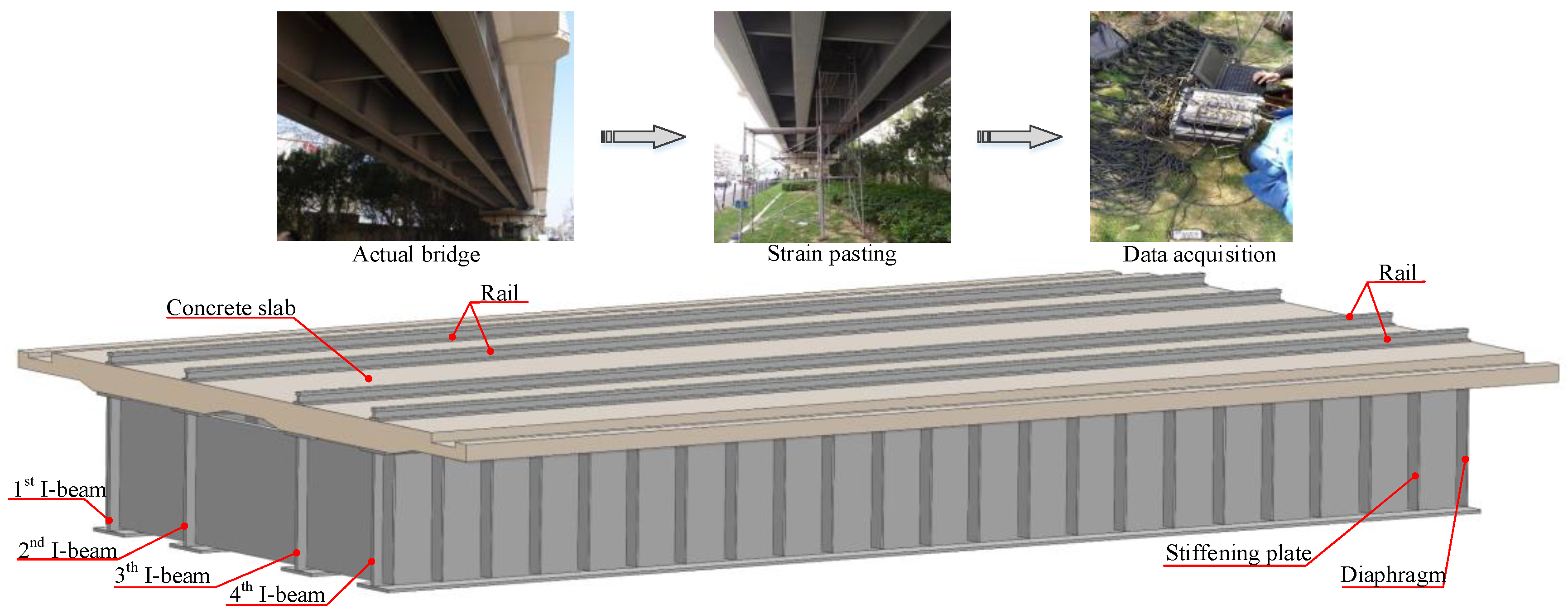
2. Structure Characterization and Field Measurement Scheme of an In-Service Simply Supported Composite Beam Bridge in Urban Rail Transit

2.1. Structure Characterization of a Simply Supported Composite Beam Bridge

This study focuses on a simply supported steel-concrete composite beam bridge located on Shanghai Metro Line 3, where on-site strain monitoring of the composite section was conducted. Built in 1997, the bridge features a structure comprising bottom I-shaped steel beams and an upper concrete slab. The standard span of the bridge is 45.0 m, with a calculated span of 44.0 m. The bottom I-beams are constructed from Q345 steel, while the upper concrete slab is composed of C40 concrete. The lower part of the composite section consists of four horizontally arranged I-beams totaling 2376 mm in height. Each I-beam web measures 2316 mm in height with a 14 mm thickness. The upper flange plate of the I-beam is 500 mm wide and 30 mm thick, while the lower flange plate is 600 mm wide and 30 mm thick. Additionally, within a 30 m range at the mid-span of the bridge, the lower flange of the composite section’s I-beams features localized thickening, with a plate width of 480 mm and a thickness of 24 mm. The upside concrete slab varies in thickness from 180 to 300 mm and spans a width of 8900 mm. Diaphragms, 2200 mm high and 12 mm thick, are installed longitudinally every 4 m between the bottom I-beams to enhance lateral connection and girder structure stability. Vertical stiffening plates, 2200 mm high, 220 mm wide, and 12 mm thick, are placed every 2 m. Figure 1 depicts the layout and cross-section diagram of the simply supported steel-concrete composite beam bridge.

Shanghai Metro Line 3 operates AC03-type trains manufactured by ALSTOM, each measuring 140 m in total length. The AC03 train configuration consists of a 6-carriage formation comprising two end locomotives (Tc) and four middle carriages (Mp). The locomotive weighs 32 t and spans 24.4 m, while each middle carriage weighs 35.65 t and measures 22.8 m in length. The train adheres to a standard lateral gauge of 1435 mm, with each carriage having a lateral width of 3.0 m. Every carriage is equipped with four axles, with each pair sharing a bogie. The long wheelbase within a single carriage is 15.7 m, and the short wheelbase is 2.5 m. The adjacent wheelbase between the two carriages is 4.6 m. Seating capacity includes 54 seats in the locomotive and 58 seats per carriage, accommodating up to 270 passengers (at 6 people/m²) when fully loaded. The composition of the AC03 train is depicted in Figure 2. To simplify the train load, the weight of each carriage is evenly distributed across its four axles. Due to the negligible difference in wheelbase between adjacent axles within the same bogie, they are merged in the train axle load model as a single calculated axle positioned at the midpoint between the two short wheels, carrying half of the carriage’s weight [24]. Consequently, the AC03 train is modeled with 12 calculated axles labeled p₁ to p₁₂ from front to back. The model assumes an even distribution of crowd load within each carriage, transmitted equally to two calculated axles per carriage. The simplified train axle load model of the AC03-type train is illustrated in Figure 2.

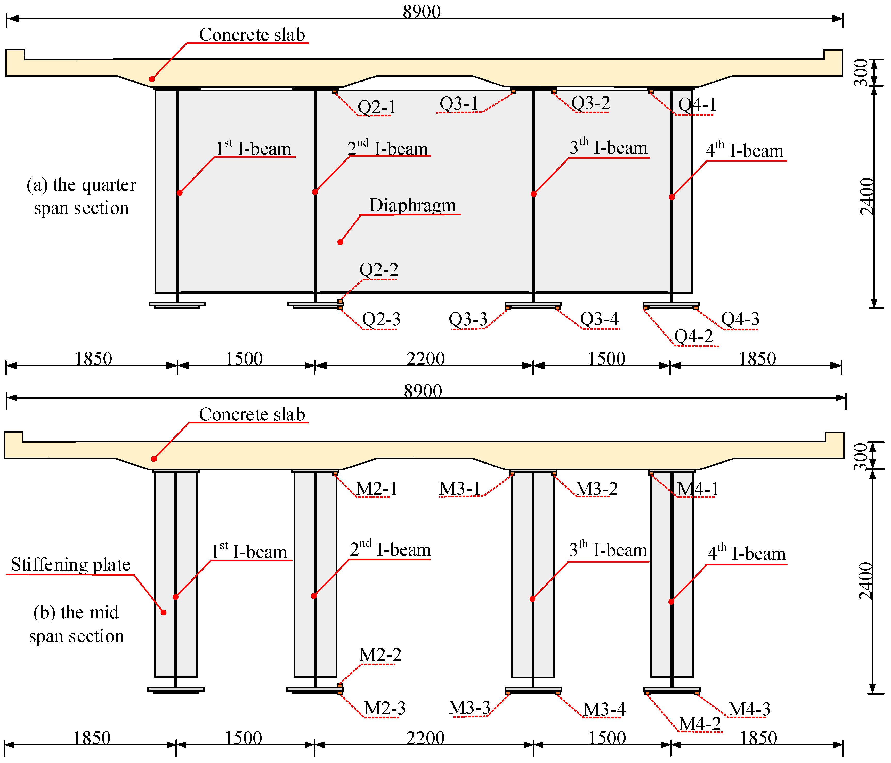
2.2. Strain Field Measurement Scheme of a Simply Supported Composite Beam Bridge

Strain measurements were conducted on the upper and lower flanges of the I-beam in the composite section of the simply supported beam bridge on Shanghai Metro Line 3. In field strain detection, due to the bridge’s simply supported structure, critical sections include the mid-span, support, and quarter-span sections, which experience the most severe stress conditions. The mid-span section bears the maximum positive bending moment, while the support section endures the maximum shear force. The quarter-span section experiences significant bending moment and shear force. Given practical constraints in deploying strain gauges, the focus was primarily on the upper and lower flanges of the I-beam in the mid-span and quarter-span sections. Figure 3 illustrates the layout and numbering of strain measurement points for these sections. The bottom I-beams of the composite girder are labeled 1st to 4th from left to right. Due to the presence of a green belt, strain measurement points were arranged on the three I-beams on the right side, omitting the 1st I-beam. Strain measurement points in the quarter-span section are denoted as Qi-j, and those in the mid-span section as Mi-j. The first digit signifies the bottom I-beam number of the composite section, while the second digit indicates the serial number of the strain gauge on the I-beam. For instance, Q2-3 denotes the third strain measurement point on the 2nd I-beam in the quarter-span section, and M2-3 denotes the third one on the 2nd I-beam in the mid-span section.

In the field strain measurement (Figure 1), two data acquisition instruments were utilized to ensure data accuracy and reliability. Specifically, strain data from the quarter-span and mid-span sections of the simply supported composite beam bridge were collected using DH 5902 and DH 5920 devices manufactured by Donghua Testing Technology. The DH 5902 data acquisition device features 32 channels and a maximum sampling frequency of 100 kHz, while the DH 5920 device includes 16 channels with a maximum sampling frequency of 128 kHz. Both devices have 16-bit A/D resolutions. Prior to strain measurement, the layout, temperature compensation, and channel connections of the strain measurement points were configured, followed by instrument calibration. During on-site strain detection, the sampling frequency of the data acquisition instruments was set to 1000 Hz, significantly exceeding twice the natural frequency of the simply supported composite beam bridge structure, thus meeting the requirements for accurate field strain detection.

The strain of the composite section of the simply supported composite beam bridge on Shanghai Metro Line 3 was monitored in situ over three days, from 27 to 29 April, including both working days and holidays. This monitoring captured the structural response of the bridge under different traffic conditions. Due to power supply constraints in outdoor settings, the data acquisition instrument was activated only when trains passed through the bridge. After filtering out abnormal data, train crossings were recorded 21, 23, and 23 times on 27, 28, and 29 March, respectively. Trains traveled in both forward and reverse directions: on 27 April, there were 12 forward and 9 reverse crossings; on 28 April, there were 12 forward and 11 reverse crossings; and on 29 April, there were 12 forward and 11 reverse crossings.

3. Numerical Modeling, Validation, and Strain Influence Lines Calculation of an In-Service Simply Supported Composite Beam Bridge

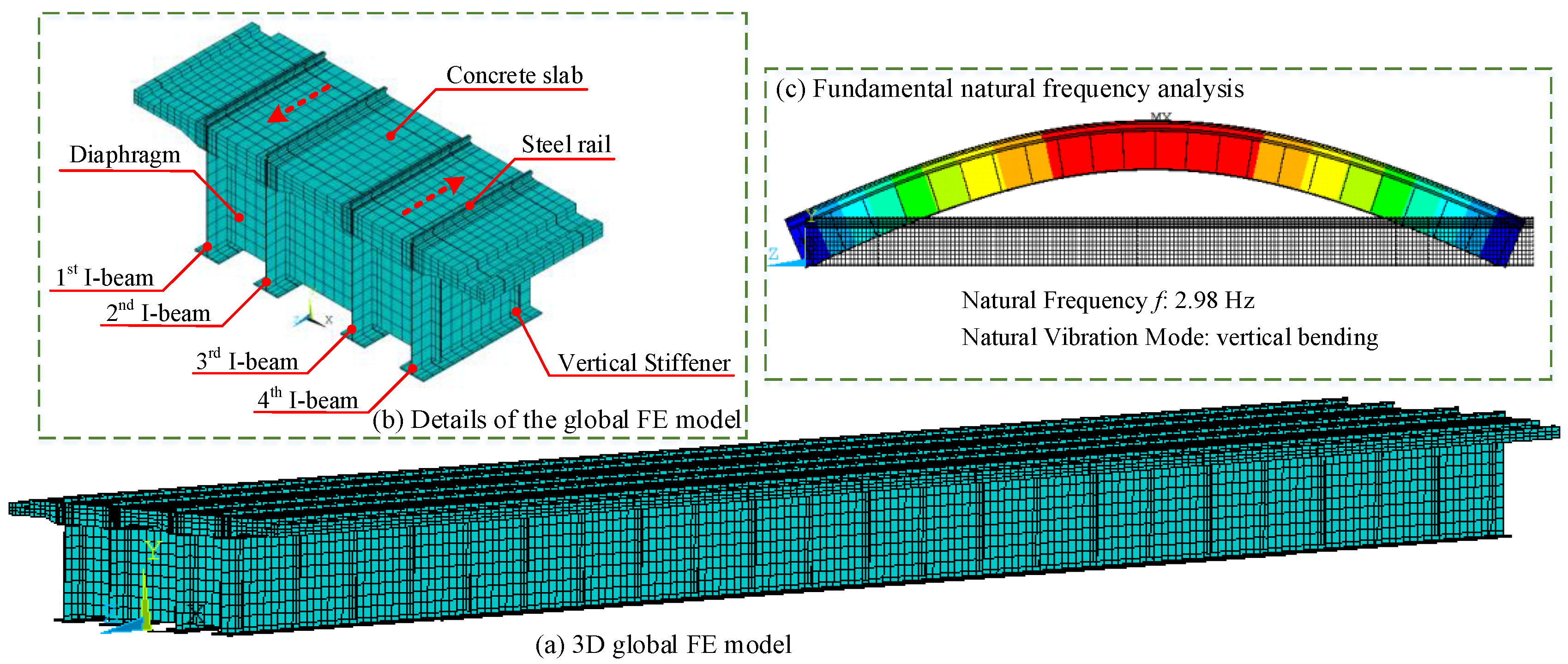
3.1. Numerical Modeling of the Simply Supported Composite Beam Bridge

The finite element (FE) software ANSYS (Version 15.0) was used to create a global model with SOLID65 and SHELL181 elements [25] for the simply supported steel-concrete composite beam bridge on Shanghai Metro Line 3. The bridge’s main components include I-beams, diaphragms, vertical stiffeners, concrete slabs, and steel rails. The upside concrete slabs of the composite section were modeled using solid elements (SOLID65), with lateral mesh sizes ranging from 150 mm to 300 mm and longitudinal mesh sizes of approximately 400 mm. The lower part of the composite section, comprising the I-beams, diaphragms, and vertical stiffening plates, was modeled using shell elements (SHELL181). The cross-sectional mesh sizes for the I-beam elements range from 100 mm to 200 mm, with longitudinal mesh sizes maintained at about 400 mm. Diaphragm and vertical stiffener elements have transverse mesh sizes between 100 mm and 300 mm, with longitudinal mesh sizes of 12 mm. The steel rails were also modeled using solid elements (SOLID65), with lateral mesh sizes ranging from 50 mm to 100 mm.

The connection between the upper flange I-beam and the concrete slabs of the composite section utilizes joint nodes of solid and shell elements to ensure a secure connection between the concrete and steel components. The boundary conditions for the global bridge model of the simply supported composite beam bridge specify that the bottom I-beam of the composite section is fixed at the left support position, restraining three degrees of freedom (global X, Y, and Z directions) at the node. Similarly, the lower I-beam of the composite section is fixed at the right support position, restricting movement in the global X and Y directions at the node. The global bridge model of the simply supported steel-concrete composite beam bridge comprises 149,976 nodes and 106,960 elements, as illustrated in Figure 4.

3.2. Validation of the Global FE Model of the Simply Supported Composite Beam Bridge

The modal properties of the simply supported composite beam bridge, specifically its natural frequencies and mode shapes, are crucial for validating the global FE model and associated numerical modeling techniques. According to the General Design Specification for Highway Bridges and Culverts [26], the fundamental natural frequency of a simply supported beam bridge can be calculated by

$$f_1={\displaystyle \frac{\pi }{2L^2}}\sqrt{{\displaystyle \frac{E{I}_c}{m_c}}}$$

(1)

where L is the calculated span of a simply supported beam bridge, E is the elastic modulus of the girder material, I_c is the moment of inertia of the girder section, and m_c is the mass per unit length of the girder. According to the composite section details of the simply supported beam bridge in Figure 3, the moment of inertia I_c and the mass per unit length m_c of the steel-concrete composite section are calculated. The theoretical value of the fundamental natural frequency of the simply supported composite beam bridge is then determined using Equation (1), yielding 3.25 Hz, corresponding to the first-order vertical bending mode of the girder. To validate the accuracy of the numerical modeling techniques employed in Section 3.3, the structural natural vibration characteristics were analyzed numerically using the established global FE model of the bridge. Through modal analysis, the fundamental natural frequency of the simply supported composite beam bridge is 2.97 Hz, which also corresponds to the first vertical bending mode of the girder (Figure 4c). The relative difference between the numerical result and the theoretical value of the first-order natural frequency is only 9.4%, which is deemed acceptable for practical engineering structures. The discrepancy may be attributed to the omission of ancillary components such as bridge deck pavement and guardrails in the theoretical calculation of the fundamental natural frequency (Equation (1)), resulting in a higher natural frequency for the simply supported composite beam bridge. In conclusion, the established global FE model of the simply supported composite beam bridge effectively captures its inherent characteristics with acceptable accuracy.

In general, the best way to validate the established numerical model of the target simply supported composite beam bridge is with the aid of experimental data, which are fully representative of the real bridge structure. Due to the busy urban traffic demand, it is impossible to stop train operations to conduct load tests on the bridge. Thus, it is not feasible to validate the numerical model based on experimental data of the bridge. As an alternative measure, the design values of the dynamic characteristics of the simply supported composite beam bridge are adopted to validate the numerical model in the above context. It should be pointed out that the dynamic behaviors calculated using stationary techniques still have a limitation for the target bridge. The target bridge in service may undergo damage over time, and its actual dynamic characteristics might be different from the design values. The validation using the design values of the dynamic characteristics of bridges thus may affect the reliability of the established numerical model to a certain extent. It might be better to employ techniques, e.g., a band-variable filter [27], which are capable of assessing non-stationary dynamic behaviors of existing structures. However, compared with the design values of structural dynamic characteristics, the techniques to capture non-stationary dynamic behaviors of existing structures are too complex in principle, and the calculation process is also very cumbersome. Hence, using design values of structural dynamic characteristics to do calibration plays a role as a quick and effective means for numerical model validation.

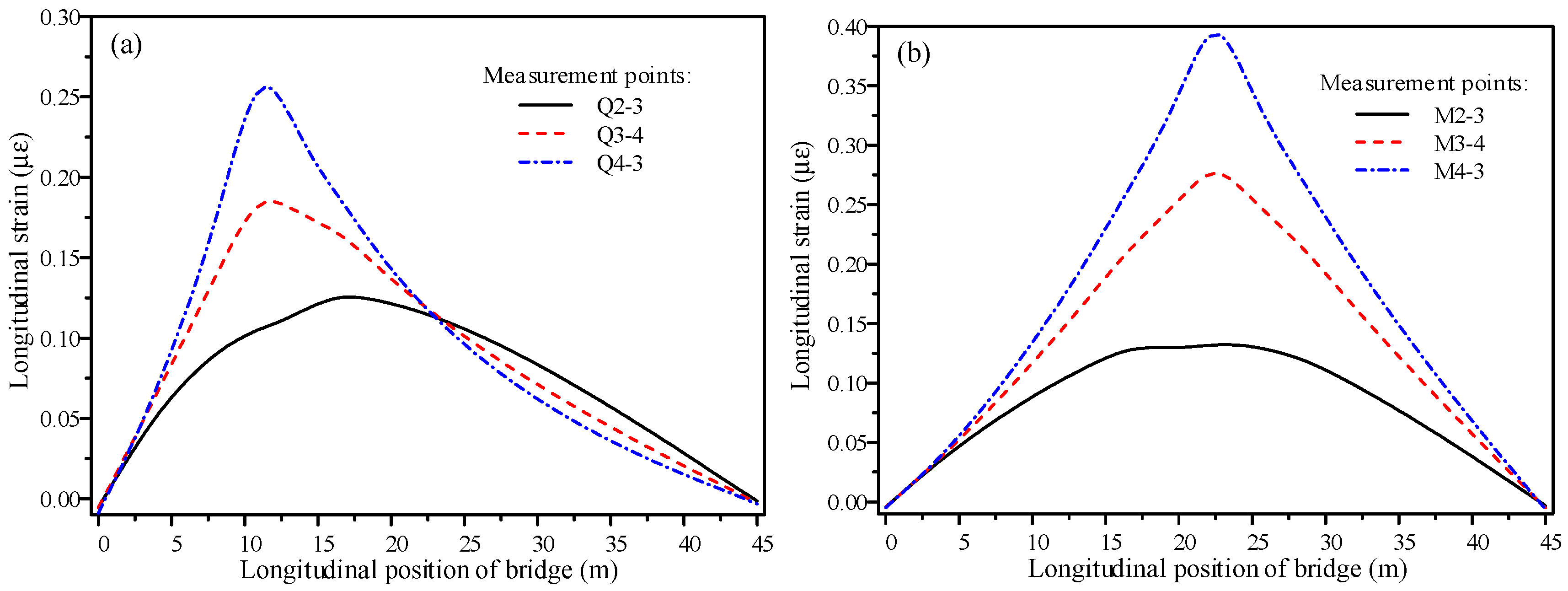
3.3. Numerical Calculation of Strain Influence Lines

The simply supported steel-concrete composite beam bridge on Shanghai Metro Line 3 operates with double-track trains traveling in both forward and reverse directions. When a concentrated unit load moves longitudinally on the rail, the longitudinal strain function at a measurement point on the composite section represents its strain influence line. The AC03 type train on the simply supported beam bridge is modeled as a series of axles with fixed spacing p_i (Figure 2). Using strain influence line theory, the effect of each axle load p_i on the bridge structure can be calculated, and the total load effect of the entire train is obtained through the superposition principle. Structural dead load effects are considered when calculating the strain influence line of the measurement points. In the validated global FE model of the simply supported composite beam bridge, vertical unit forces of 1.0 kN are applied on the steel rail along the longitudinal direction of the girder for analysis. Figure 5 illustrates the longitudinal strain influence lines of six measurement points (Q2-3, Q3-4, Q4-3, M2-3, M3-4, M4-3) located on the quarter and mid-span sections of the simply supported composite beam bridge in the forward direction. From Figure 5a, it is evident that the longitudinal strain influence lines of the three measurement points on the bottom plate of the I-beam at the quarter-span exhibit a single-peak shape. The strains at these points peak when the moving unit load is near the quarter-span (x = 11.25 m) in the longitudinal direction, with peak strains around 0.26 με, 0.18 με, and 0.13 με, respectively. Additionally, the peak strain at measurement point Q4-3 slightly lags behind the other two points, likely due to its location on the outermost I-beam. Figure 5b shows the longitudinal strain influence lines of three measurement points on the bottom plate of the I-beam at the mid-span section, also displaying a unimodal shape. The strains at these points reach their peak values when the moving load is near the mid-span (x = 22.5 m), with peak strains approximately 0.39 με, 0.28 με, and 0.13 με, respectively.

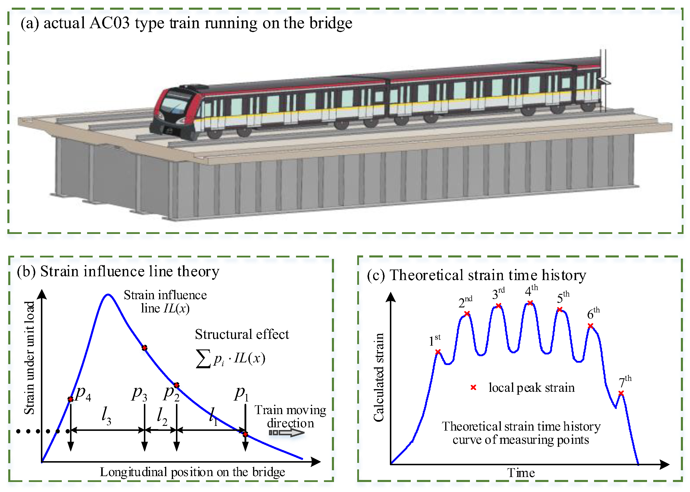
4. Identification Method of Train Axle Loads Using Strain Influence Line Theory with Mathematical Optimization Techniques

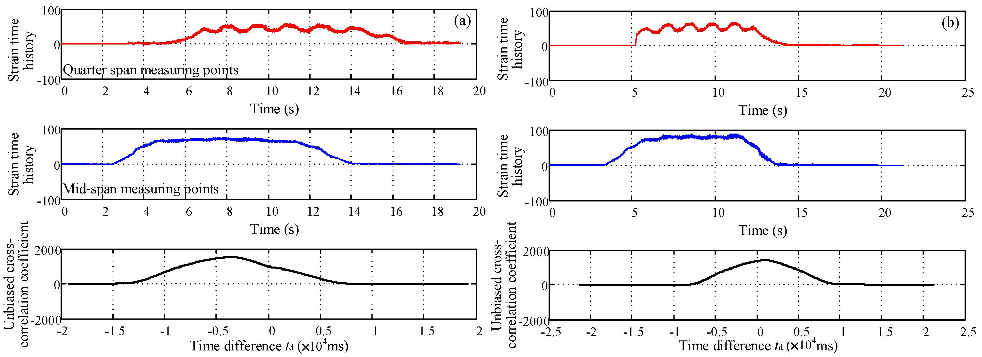
4.1. Train Speed Estimation

In this study, the signal cross-correlation function [28] was employed to estimate the speed of trains traveling across the simply supported composite beam bridge on Shanghai Metro Line 3. When a train passes through the quarter and mid-spans of the bridge, longitudinal strain time histories from corresponding measurement points on these sections are monitored (Figure 3). From a signal analysis perspective, there exists a correlation between the strain time history curves of corresponding measurement points at the quarter and mid-span sections under the same train. The correlation coefficient R quantifies the degree of correlation between strain values of the corresponding measurement points at the quarter-span ${\epsilon }_{i-j}^Q(t)$ and mid-span ${\epsilon }_{i-j}^M(t)$ sections at any given time t and t + τ. The cross-correlation function R(τ) between these strain time series at a time difference τ can be computed using the equation

$$R(\tau )={\displaystyle {\int }_{-\infty }^{\infty }{\epsilon }_{i-j}^Q(t){\epsilon }_{i-j}^M(t+\tau )}$$

(2)

According to the cross-correlation function, when a train sequentially passes through the quarter and mid-spans of the simply supported composite beam bridge, the cross-correlation function R(τ) of the strain time history ${\epsilon }_{i-j}^Q(t)$ and ${\epsilon }_{i-j}^M(t)$ at the corresponding measurement points reaches its maximum at the time difference τ = t_d. This indicates that the strain time history ${\epsilon }_{i-j}^M(t)$ from the mid-span section, when shifted forward by time t_d, most closely matches the strain history ${\epsilon }_{i-j}^Q(t)$ from the quarter-span section. The cross-correlation coefficient of strain time histories at corresponding measurement points is calculated for each train passing through the quarter and mid-spans of the bridge to determine the time difference t_d at which the cross-correlation coefficient reaches its maximum value. The average speed v_t of each train passing through the bridge is estimated using the ratio of the distance L/4 between the quarter and mid-span sections to the time difference t_d. When a train passes through the simply supported composite beam bridge at speed v_t, the on-site measured strains at the quarter and mid-span sections both include dynamic amplification effects. For urban rail transit bridges, the dynamic amplification effect is generally calculated by multiplying the vertical static load effect of the train by a dynamic amplification coefficient μ. The dynamic amplification factor μ is determined by the train speed v_t and the bridge span L. For urban rail transit trains traveling at speeds generally below 80 km/h, the dynamic amplification factor μ is 0.8 times that specified for railway bridges. According to the Design Specification for Railway Bridges and Culverts [29], the dynamic amplification factor μ of the simply supported steel-concrete composite beam bridge for urban rail transit with a span of L can be obtained by

$$1+\mu =1+0.8\times {\displaystyle \frac{22}{40+L}}$$

(3)

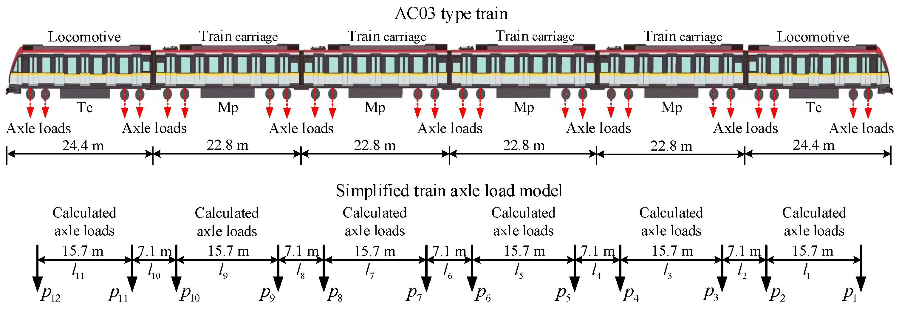
4.2. Train Axle Loads Identification

The identification of train axle loads for the AC03 type train operating on Shanghai Metro Line 3 involves solving an inverse structural response problem. In this method, the known structural responses (strain measurements) are used to determine the axle loads that cause these responses. This approach is rooted in strain influence line theory, where the effect of a specific axle load is proportional to the product of the influence line ordinate and the magnitude of the axle load at the corresponding position. The AC03 type train configuration (Figure 2) and its operational speed on Shanghai Metro Line 3 have been established. The unknowns in this context are solely the axle loads of the AC03 train, denoted as P = [p₁ p₂ … p_Na]^T, where p_i represents the load of the train axle i, and N_a is the total number of train axles. Therefore, theoretically, the axle loads p_i (i = 1 to N_a) can be determined by N_a time’s measurement of the structural responses (strain measurement) at distinct N_a longitudinal positions.

As depicted in Figure 6a, the given AC03 type train on Shanghai Metro Line 3 travels across the simply supported composite beam bridge at a velocity of v_t. Time is designated as 0 when the first train axle of the AC03 type train enters the bridge. At time t, the train will arrive at the longitudinal position x = v_tt. At any given longitudinal position x, the coefficient matrix I(x) representing the strain influence line for all the strain measurement points is

$$\mathbf{I}(x)={\left[\begin{array}{cccc}I{L}_1(x)& I{L}_1(x-l_1)& \cdots & I{L}_1(x-{\displaystyle {\sum }_{k=1}^{N_a}{l}_k})\\ I{L}_2(x)& I{L}_2(x-l_1)& \cdots & I{L}_2(x-{\displaystyle {\sum }_{k=1}^{N_a}{l}_k})\\ ⋮& ⋮& \ddots & ⋮\\ I{L}_{N_m}(x)& I{L}_{N_m}(x-l_1)& \cdots & I{L}_{N_m}(x-{\displaystyle {\sum }_{k=1}^{N_a}{l}_k})\end{array}\right]}_{N_m\times N_a}$$

(4)

where IL_i(x) represents the strain influence line function for measurement point i, as detailed in Section 4.1. The coefficient matrix I(x) of the strain influence line is an N_m × N_a matrix, where each element IL_i(x) is determined by the longitudinal position of each axle of the AC03 type train along with the strain influence line for measurement point i. The N_m denotes the total number of strain measurement points on the simply supported composite beam bridge (Figure 3). The l_k signifies the distance between the first and the k-th axle of the AC03-type train. Based on the calculated strain influence lines (Figure 2), the theoretical strains ${\mathsf{\epsilon }}^c\left(t\right)$ at all strain measurement points at time t can be derived relative to the longitudinal position x of the first train axle using

$${\mathbf{\epsilon }}^c(t)={[{\epsilon }_1^t {\epsilon }_2^t \cdots {\epsilon }_{N_m}^t]}^T=I(t)\times P$$

(5)

The theoretical strains ${\mathsf{\epsilon }}^c\left(t\right)$ form a column vector that includes the calculated strain values at all measurement points at time t. Therefore, based on Equation (5), it becomes feasible to establish a system comprising N_a equations with N_a unknowns by selecting N_a positions for the first train axle. This approach facilitates the determination of the axle loads p_i for the given AC03 type train. In practical scenarios involving on-site strain measurements on actual bridges, the number of data samples collected is typically much greater than N_a, owing to continuous strain data acquisition by the measurement system. This data abundance ensures a robust basis for accurate train axle load identification.

When a train travels a simply supported beam bridge, the strain time history curves at each measurement point typically exhibit a multi-peak shape, as shown in Figure 6c. This characteristic arises because each axle of the train induces strain responses as it moves along the bridge. The number and magnitude of these local peak strains in the strain time history are directly influenced by the train axle load vector P and the strain influence line IL_i(x) of the measurement point i. In practical engineering applications, there often exists a discrepancy between the theoretical strains and the actual strains measured on-site at specific measurement points on simply supported composite beams. Thus, taking the local peak strain in the strain time history curve into consideration, the axle loads identification of the given AC03 type train is carried out by minimizing the quadratic difference between the theoretical calculated and on-site measured local peak strains for the measurement point i, which is defined by

$$e_i={\displaystyle \sum _{j=1}^{N_j}{\left({\epsilon }_j^{pc}-{\epsilon }_j^{pm}\right)}^2}$$

(6)

where the ${\epsilon }_j^{pc}$ is the theoretically calculated j-th local peak strain, while the ${\mathsf{\epsilon }}_j^{pm}$ is the on-site measured j-th local peak strain for the measurement point i. The N_j is the total number of the local peak strains in the strain time history curve of the measurement point i. The minimization of Equation (6) utilizes a genetic algorithm known for its effectiveness in searching the global optimum across various optimization problems. This includes scenarios where the objective function is discontinuous, non-differentiable, stochastic, or highly nonlinear [30,31]. The genetic algorithm initiates with multiple feasible solutions P_i (i = 1 to N_s, i∈N⁺), each represented as an individual in the form of a binary string. These multiple feasible solutions P_i constitute a population, with a size N_s of 60 tailored to address the optimization problem defined in Equation (6). The algorithm iteratively applies selection, crossover, and mutation operators to generate successive generations, guiding the population toward an optimal solution. A crossover ratio of 1.0 is maintained to preserve sufficient variability in the next population. Consequently, the global optimum solution P_b = [$p_1^b$ $p_2^b$… $p_{N_a}^b$]^T for the axle loads of the AC03 type train is determined. The crossover ratio is set to 1.0 to keep adequate variability for the next population. The global optimum solution P_b = [$p_1^b$ $p_2^b$… $p_{N_a}^b$]^T for the axle loads of the given AC03 type train is thus finally determined. Based on the AC03 type train passing over the simply supported composite beam bridge at speed v_t, the strain responses at each measurement point incorporate dynamic impact effects. These effects are adjusted by the dynamic amplification factor μ specific to each train (Equation (3)), as derived in Section 4.2. Therefore, the actual axle loads of the AC03-type train are ultimately represented by

$$P={\displaystyle \frac{1}{1+\mu }}{P}_b={\displaystyle \frac{1}{1+\mu }}{[p_1^b p_2^b \cdots p_{N_a}^b]}^T$$

(7)

According to the measured strain time history of each measurement point, the train axle load vector P_b = [$p_1^b$ $p_2^b$… $p_{N_a}^b$]^T can be derived. The simply supported composite beam bridge features a total of N_m strain measurement points located on the quarter and mid-span sections (Figure 3). Utilizing the redundant on-site measured strain time histories from these points allows for the computation of multiple estimations of the train axle load vector P_b for the AC03 type train. To obtain the final values p_i (i = 1 to N_a), representing individual axle loads, the average of all previous estimations is calculated, therefore mitigating potential outliers. The method outlined above facilitates the calculation of each axle load by correlating measured strains with established strain influence lines. This correlation provides essential data for evaluating the structural performance and ensuring the operational safety of the bridge under dynamic train loads.

5. Application of Train Axle Loads Identification Method

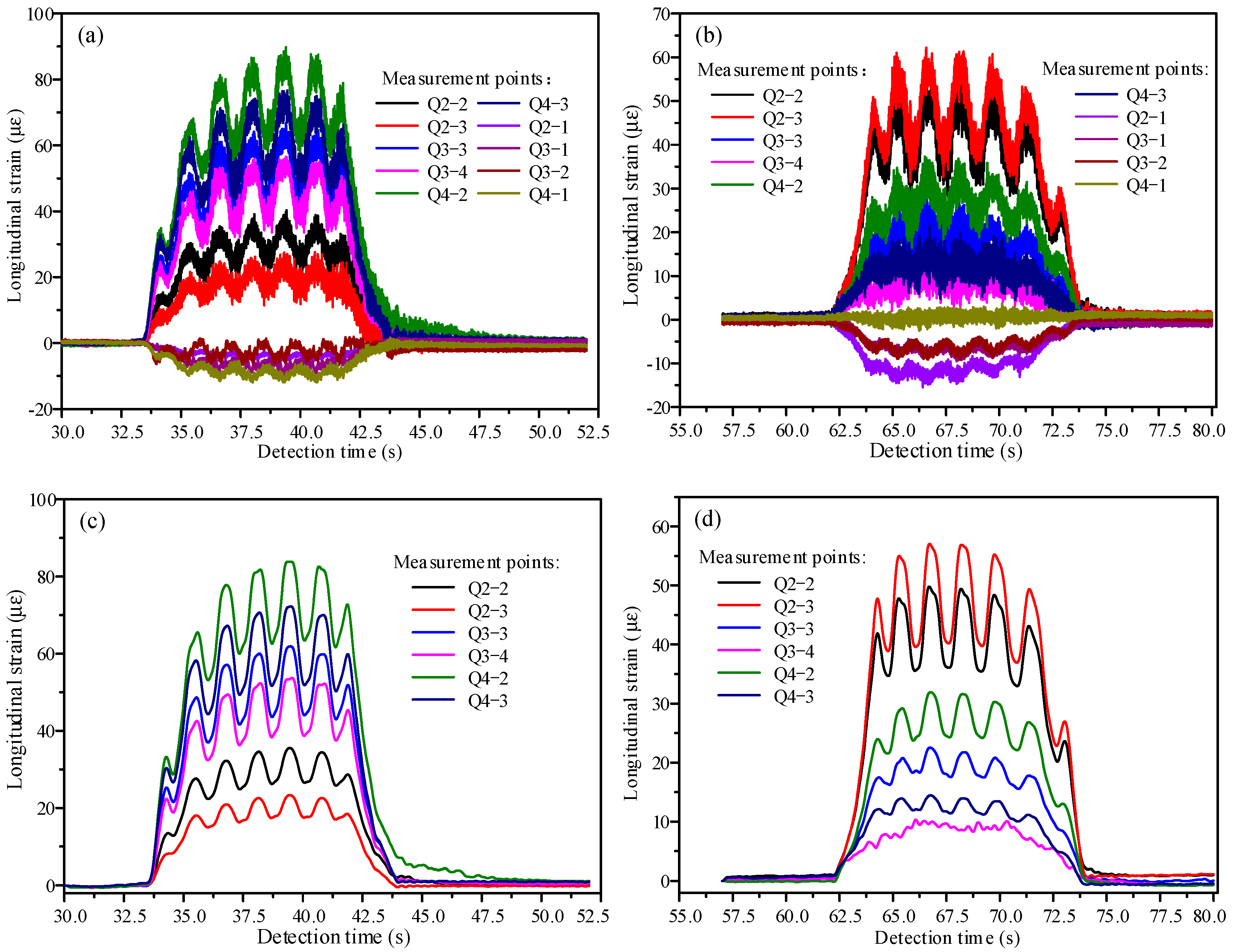
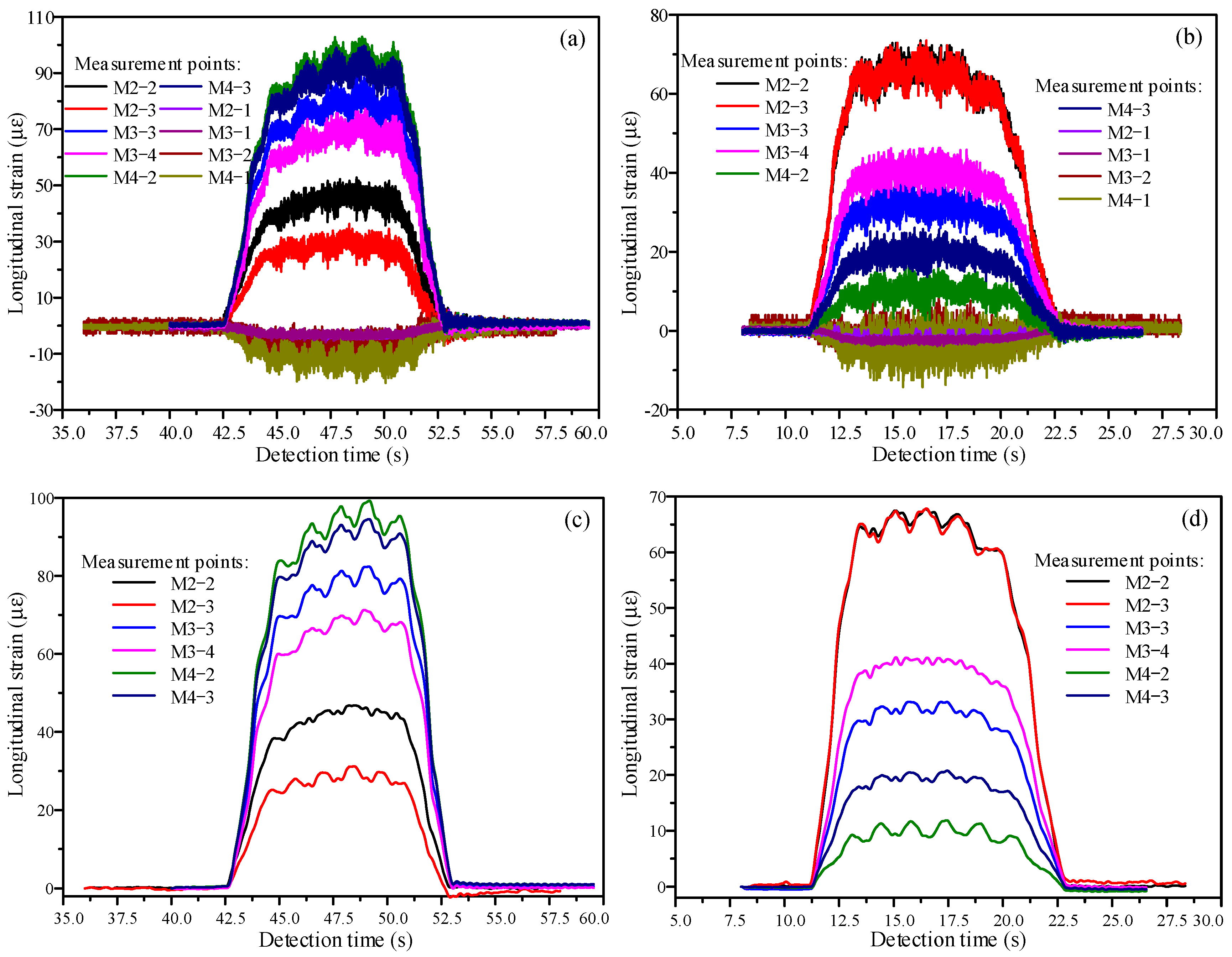
5.1. Pre-Processing of Strain Measurement Data

The strain time history curves from 20 measurement points located at the quarter and mid-span sections of the simply supported composite beam bridge were continuously recorded by the data acquisition instrument for each passing train. The strain measurement data were found to contain high-frequency environmental noise (Figure 7a,b and Figure 8a,b). To mitigate this noise, a Butterworth low-pass filter was employed. The Butterworth filter is characterized by a smooth frequency response in the passband and a gradual attenuation in the stopband. In MATLAB software (Version 2012a), the passband cutoff frequency of the Butterworth low-pass filter was set to 2.2/1000 (normalized at 1000 Hz), while the stopband cutoff frequency was set to 4.4/1000 (normalized at 1000 Hz). The passband and stopband attenuations were configured as 0.1 and 2.2, respectively. Additionally, since strain data from measurement points on the quarter and mid-span sections were collected using two separate data acquisition devices, inconsistencies in total duration and amount of time history data arose. To synchronize these data-sets, zero-point filling was applied before and after the strain time series. Following these pre-processing steps, the strain time history curves for the quarter and mid-span measurement points of the simply supported composite beam bridge are presented in Figure 7c,d, and Figure 8c,d.

The typical strain time history curve of the quarter-span strain measurement points on the simply supported composite beam bridge is depicted in Figure 7. At these points, both ends of the strain time history curve exhibit steady fluctuations before and after the passage of a train. During the train’s traversal across the bridge, the strain time history curve shows seven local peaks, with the middle five peaks being more pronounced and the outermost two slightly smaller. Some measurement points may exhibit less pronounced peaks on both sides. Regarding peak strain, during the passage of a forward train (Figure 7a,c), the maximum measured strain in the strain time history curve occurs at measurement point Q4-2 on the bottom flange of the far-right I-beam, reaching approximately 85 με. The strain peaks decrease as the measurement points approach the opposite side. Conversely, when a train moves in reverse (Figure 7b), the highest peak strain is observed at measurement point Q2-3 on the bottom flange of the second I-beam, with a magnitude of about 60 με. Similarly, the strain peaks decrease as the measurement points approach the positive side. Additionally, strain values on the upper flange of the I-beam generally exhibit smaller peak strains and experience compressive stress.

The typical strain time history curve of measurement points at the mid-span of the simply supported composite beam bridge is depicted in Figure 8. At these mid-span measurement points, both ends of the strain time history curve exhibit steady fluctuations before and after the train passes over the bridge. In contrast to the quarter-span measurement points, the strain time history curve during the passage of a forward train shows only 5 local peaks. Conversely, during the passage of a reverse train, the peaks and valleys of the strain time history curve at mid-span measurement points are less pronounced. Regarding peak strain, during the passage of a forward train (Figure 8a,c), the maximum measured strain in the strain time history curve occurs at measurement point M4-2 on the bottom flange of the far-right I-beam, reaching approximately 97 με. The strain peaks decrease as the measurement points approach the opposite side. Conversely, when a reverse train passes (Figure 8b), the highest peak strains are observed at measurement points M2-2 and M2-3 on the bottom flange of the second I-beam, with magnitudes of about 70 με. Similarly, the strain peaks decrease as the measurement points approach the positive side. Additionally, strain values on the upper flange of the I-beam generally exhibit smaller peak strains and typically experience compressive stress.

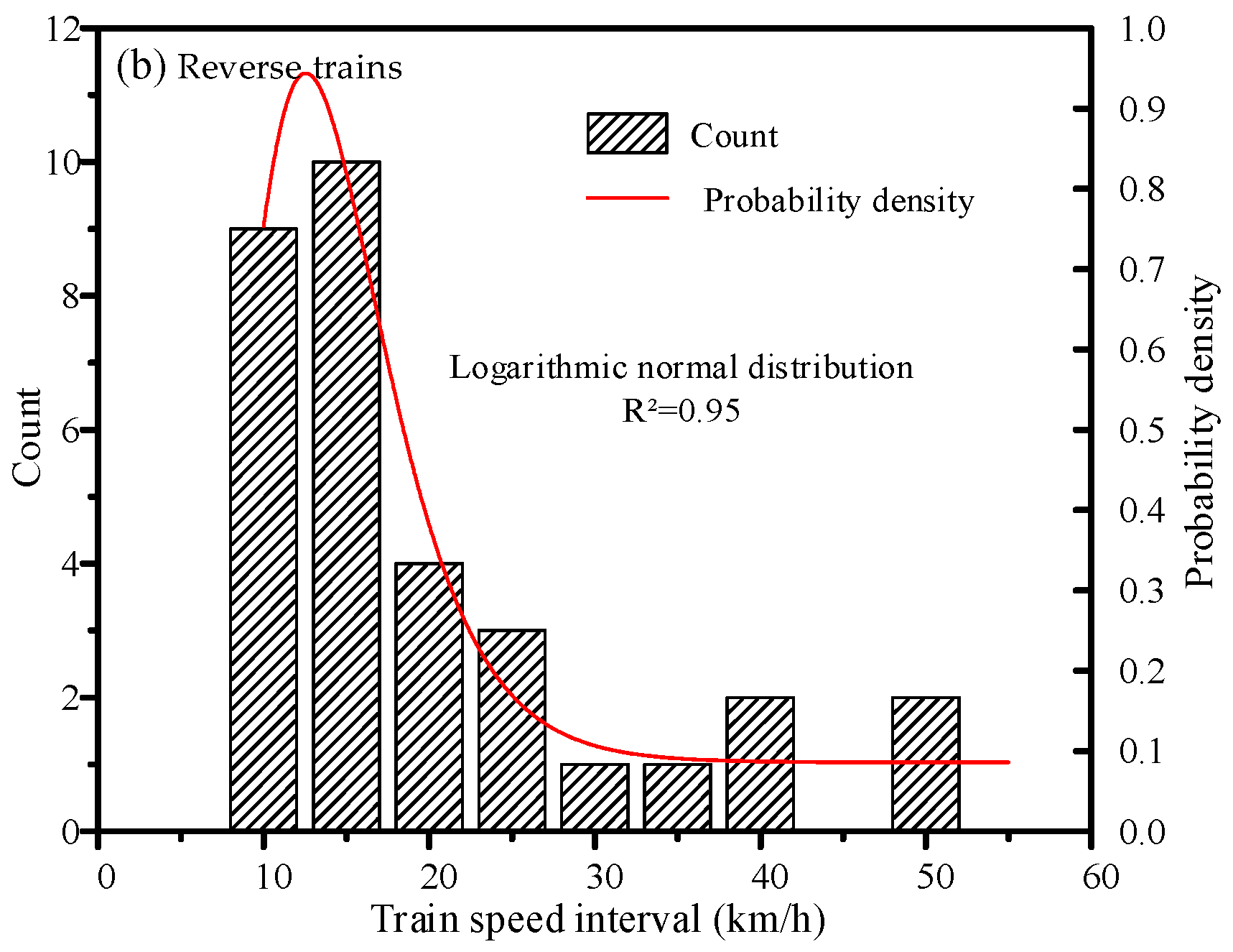
5.2. Train Speed Analysis for Urban Rail Transit

The train speeds on the simply supported composite beam bridge of Shanghai Metro Line 3 were estimated using signal cross-correlation functions, as detailed in Section 4.1. Taking the 2nd train (reverse direction) and the 12th train (forward direction) on April 27th as examples, after data pre-processing, the strain time history curves and cross-correlation functions of corresponding measurement points on the quarter and mid-span sections of the bridge are illustrated in Figure 9. The cross-correlation function on the horizontal axis ranges symmetrically about zero time, encompassing both positive and negative values, indicating the time difference between the two signals. The time difference t_d corresponding to the maximum cross-correlation value represents the time taken for the train to travel between the quarter and mid-span sections of the bridge. From Figure 10a, it is observed that the time difference t_d is 3.46 s when the cross-correlation function of the strain time history signal reaches its maximum value. Therefore, the average speed of the 2nd train crossing the bridge is v_t = L/(4t_d) = 11.68 km/h. Similarly, according to Figure 10b, the time difference t_d is 1.05 s, and the corresponding cross-correlation function reaches its maximum value. Thus, the average speed of the 12th train crossing the bridge is v_t = L/(4t_d) = 38.48 km/h.

For other detected trains, the cross-correlation function method was also employed to analyze their average travel speeds. The resulting histogram depicting the travel speed distribution of a total of 68 trains (36 in the forward direction and 32 in the reverse direction) is presented in Figure 10. The speed distribution of trains on Shanghai Metro Line 3 shows a certain degree of dispersion. Both forward and reverse train speeds follow a logarithmic normal distribution, with R² values of 0.95 for both directions. Specifically, the speed range for forward trains is 8.9 to 82.5 km/h (Figure 10a), whereas reverse trains exhibit speeds ranging from 10.8 to 55 km/h (Figure 10b). The dispersion of speeds among forward trains is relatively large, with a variance of 341.4, likely due to acceleration as trains depart from nearby stations. In contrast, reverse trains show comparably less variance at 136.5, reflecting braking and deceleration as they approach the station. The statistical mean speed for forward trains is 29.2 km/h, while for reverse trains, it is 22.5 km/h. This difference is attributed to the braking deceleration stage of reverse trains near the station. Overall, the speed distributions observed for both forward and reverse trains on Shanghai Metro Line 3 are deemed reasonable.

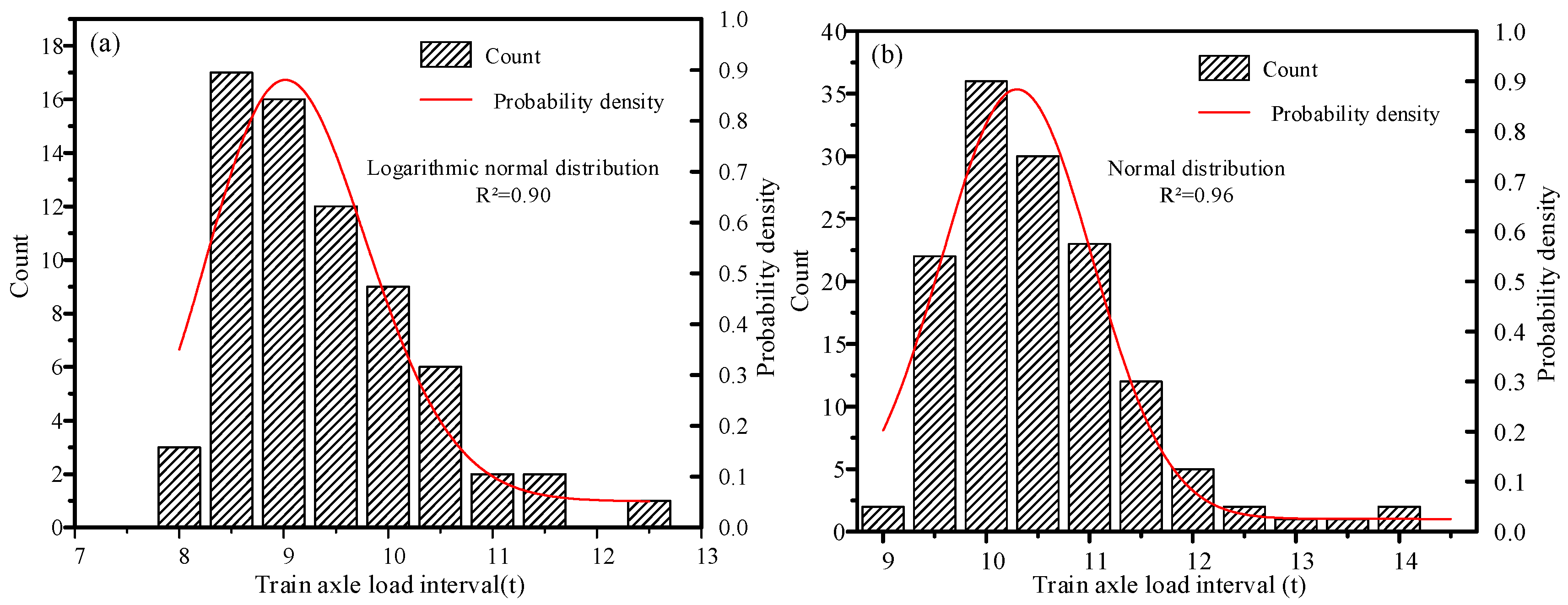
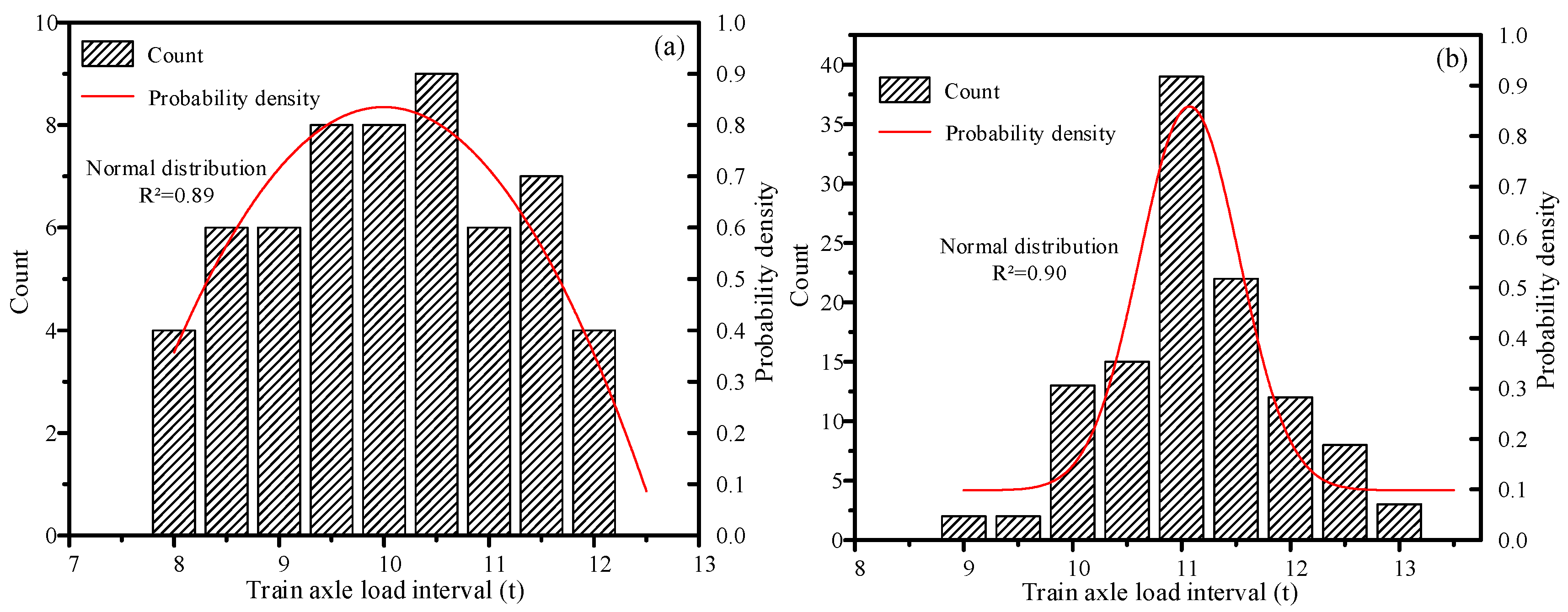
5.3. Train Axle Load Analysis for Urban Rail Transit

The axle loads of a total of 68 trains traveling on the simply supported composite beam bridge of Shanghai Metro Line 3 were identified and analyzed. Histograms depicting the axle loads of locomotives (Tc) and middle train carriages (Mp) for forward trains are shown in Figure 11. There is a certain degree of dispersion in the axle loads of locomotives and middle train carriages for forward trains. The axle loads of locomotives for forward trains follow a logarithmic normal distribution characterized by an R² value of 0.89. Specifically, the axle load range for locomotives of forward trains is 8.0 to 12.5 t (Figure 11a), with a statistical mean of 9.64 t and a variance of 0.8. Similarly, the axle loads of middle train carriages for forward trains exhibit a normal distribution, with an R² value of 0.95. The axle load range for middle train carriages of forward trains spans 9.0 to 14.5 t (Figure 11b), with a statistical mean of 10.77 t and a variance of 0.8. Notably, the mean axle load of middle train carriages is higher than that of locomotives for forward trains, which is consistent with passenger traveling habits, as well as the functional settings of different train carriages. The equal variance values of axle loads between locomotives and middle train carriages for forward trains suggest comparable variability in passenger loads across these compartments during operations. Overall, considering the train design configuration (Figure 2) and relevant literature [32], the mean values and distributions of axle loads for locomotives (Tc) and middle train carriages (Mp) for forward trains on Shanghai Metro Line 3 are reasonable.

The histograms displaying the axle loads of locomotives (Tc) and middle train carriages (Mp) for reverse trains traveling on the simply supported composite beam bridge of Shanghai Metro Line 3 are presented in Figure 12. There is a noticeable degree of dispersion in the axle loads of both locomotives and middle train carriages for reverse trains. The axle loads of locomotives for reverse trains follow a normal distribution, characterized by an R² value of 0.89. Specifically, the axle load range for locomotives of reverse trains spans from 8.0 to 12.5 t (Figure 12a), with a statistical mean of 10.28 t and a variance of 1.36. Similarly, the axle loads of middle train carriages for reverse trains also exhibit a normal distribution, with an R² value of 0.90. The axle load range for middle train carriages of reverse trains falls between 9.0 and 14.5 t (Figure 12b), with a statistical mean of 10.77 t and a variance of 0.8. Interestingly, unlike forward trains, the mean values of axle loads for locomotives and middle train carriages in reverse trains are nearly consistent. Furthermore, the variance of axle loads for locomotives is larger than that of middle train carriages for reverse trains, indicating significant variability in passenger loads in locomotives during operations. In light of justifications from the train design configuration (Figure 2) and relevant literature [32], the mean values and distributions of axle loads for locomotives (Tc) and middle train carriages (Mp) in reverse trains on Shanghai Metro Line 3 are also reasonable.

6. Conclusions and Discussion

This research introduces a novel method for identifying train axle loads considering dynamic amplification effects, utilizing a hybrid approach combining strain influence line theory and mathematical optimization. The methodology was applied to an in-service simply supported composite beam bridge within an urban rail transit system. A dedicated strain field measurement scheme was developed and implemented, facilitating comprehensive data acquisition. Numerical modeling and validation were integral parts of this study, particularly in establishing and verifying the strain influence lines at measurement points across the bridge. Statistical analyses were performed on the distribution patterns of train axle loads within urban rail transit scenarios. According to the above comprehensive analysis, the following conclusions can be drawn:

(1) The axle load characteristics of forward AC03-type trains on Shanghai Metro Line 3 exhibit distinct statistical distributions: locomotives follow a logarithmic normal distribution model, whereas middle train carriages conform to a normal distribution model. Specifically, the statistical mean value of axle load of locomotives is 9.64 t, while it is 10.77 t for middle train carriages. The axle load of locomotives and middle train carriages has the same variance with values of 0.8.

(2) The axle loads of locomotives and middle train carriages for reverse AC03 type trains on Shanghai Metro Line 3 both follow normal distribution models. The statistical findings indicate that both locomotives and middle train carriages of reverse trains have similar mean axle loads of around 10.5 t. However, there is a notable difference in variance, with locomotives exhibiting higher variability (variance of 1.36) compared to middle train carriages (variance of 0.8).

(3) The developed method for identifying train axle loads, which considers dynamic amplification effects through a hybrid approach combining strain influence line theory and mathematical optimization, proves effective in monitoring train loads and assessing their impact on structural integrity.

Although the train axle load identification method developed in the study is based on a simply supported beam bridge and applied to AC03 type train, the methodology itself has strong scalability due to the universality of the two inside basic principles of strain influence line theory and mathematical optimization techniques. For different bridge types, such as continuous beam bridges, arch bridges, and cable-stayed bridges, it is only necessary to calculate strain influence lines of measurement points in a targeted manner to update the coefficient matrix I(x) (Equation (4)). For different trains, only the axle load matrix P needs to be adjusted according to the specific train configuration.

Currently, due to limitations in measurement data size, the analysis of train axle load distribution is restricted to locomotives and middle train carriages. Moving forward, an ongoing collection of strain responses at measurement points on the simply supported composite beam bridge will be conducted to expand the sample data size. This expansion aims to establish comprehensive axle load distribution models for each carriage type on Shanghai Metro Line 3.

In the near future, based on the developed method and artificial intelligence technology, the intelligent identification and overload warning system for train axle loads will be designed and installed on the simply supported composite beam bridge on Shanghai Metro Line 3. By accurately determining train axle loads and providing timely overload warnings, engineers can effectively assess the bridge’s response to dynamic loading conditions, therefore enhancing the safety and longevity of existing bridge structures.

References

1. Wu, P.B.; Zhang, F.B.; Wang, J.B.; Wei, L.; Huo, W.B. Review of wheel-rail forces measuring technology for railway vehicles. Adv. Mech. Eng. 2023, 15, 1–15. [Google Scholar] [CrossRef]
2. Chen, Q.H.; Gong, J.C.; Ge, X.; Chen, S.Q.; Wang, K.Y. Estimation of wheel-rail forces based on the STF-SCKF-NE algorithm. Measurement 2024, 236, 114974. [Google Scholar] [CrossRef]
3. Mao, J.X.; Zhu, X.J.; Wang, H.; Guo, X.M.; Pang, Z.H. Train Load Identification of the Medium-Small Railway Bridge using Virtual Axle Theory and Bayesian Inference. Int. J. Struct. Stab. Dyn. 2024, 24, 2450193. [Google Scholar] [CrossRef]
4. Kanehara, H.; Fujioka, T. Measuring rail/wheel contact points of running railway vehicles. Wear 2002, 253, 275–283. [Google Scholar] [CrossRef]
5. Matsumoto, A.; Sato, Y.; Ohno, H.; Tomeoka, M.; Matsumoto, K.; Kurihara, J.; Ogino, T.; Tanimoto, M.; Kishimoto, Y.; Sato, Y.; et al. A new measuring method of wheel–rail contact forces and related considerations. Wear 2008, 265, 1518–1525. [Google Scholar] [CrossRef]
6. Gullers, P.; Andersson, L.; Lundén, R. High-frequency vertical wheel-rail contact forces-field measurements and influence of track irregularities. Wear 2008, 265, 1472–1478. [Google Scholar] [CrossRef]
7. Urda, P.; Muñoz, S.; Aceituno, J.F.; Escalona, J.L. Wheel-rail contact contact force measurement using strain gauges and distance lasers on a scaled railway vehicle. Mech. Syst. Signal Process. 2019, 138, 106555. [Google Scholar] [CrossRef]
8. Jin, X.C. A measurement and evaluation method for wheel-rail contact forces and axle stresses of high-speed train. Measurement 2020, 149, 106983. [Google Scholar] [CrossRef]
9. Zhou, W.; Abdulhakeem, S.; Fang, C.C.; Han, T.H.; Li, G.F.; Wu, Y.T.; Faisal, Y. A new wayside method for measuring and evaluating wheel-rail contact forces and positions. Measurement 2020, 166, 108244. [Google Scholar] [CrossRef]
10. Peng, X.Y.; Zeng, J.; Wang, J.B.; Wang, Q.S.; Li, D.D.; Liang, S.K. Wayside wheel-rail vertical contact force continuous detecting method and its application. Measurement 2022, 193, 110975. [Google Scholar] [CrossRef]
11. Roveri, N.; Carcaterra, A.; Sestieri, A. Real-time monitoring of railway infrastructures using fibre bragg grating sensors. Mech. Syst. Signal Process. 2015, 60–61, 14–28. [Google Scholar] [CrossRef]
12. Gao, L.; Zhou, C.Y.; Xiao, H.; Chen, Z.P. Continuous vertical wheel-rail force reconstruction method based on the distributed acoustic sensing technology. Measurement 2022, 197, 111297. [Google Scholar] [CrossRef]
13. Uhl, T. The inverse identification problem and its technical application. Arch. Appl. Mech. 2007, 77, 325–337. [Google Scholar] [CrossRef]
14. Pau, A.; Vestroni, F. Weigh-in-motion of train loads based on measurements of rail strains. Struct. Control Health Monit. 2021, 28, e2818. [Google Scholar] [CrossRef]
15. Marques, F.; Moutinho, C.; Hu, W.H.; Cunha, A.; Caetano, E. Weigh-in-motion implementation in an old metallic railway bridge. Eng. Struct. 2016, 123, 15–29. [Google Scholar] [CrossRef]
16. Wang, H.; Zhu, Q.X.; Li, J.; Mao, J.X.; Hu, S.T.; Zhao, X.X. Identification of moving train loads on railway bridge based on strain monitoring. Smart Struct. Syst. 2019, 23, 263–278. [Google Scholar]
17. Deepthi, T.M.; Saravanan, U.; Prasad, A.M. Algorithms to determine wheel loads and speed of trains using strains measured on bridge girders. Struct. Control Health Monit. 2019, 26, e2282. [Google Scholar] [CrossRef]
18. Wang, Y.; Qu, W.L. Moving train loads identification on a continuous steel truss girder by using dynamic displacement influence line method. Int. J. Steel Struct. 2011, 11, 109–115. [Google Scholar] [CrossRef]
19. Wang, Y.; Qu, W.L.; Xiao, C. Moving train loads and parameters identification on a steel truss girder model. Int. J. Steel Struct. 2015, 15, 165–173. [Google Scholar] [CrossRef]
20. Sekuła, K.; Kołakowski, P. Piezo-based weigh-in-motion system for the railway transport. Struct. Control Health Monit. 2012, 19, 199–215. [Google Scholar] [CrossRef]
21. Pimentel, R.; Ribeiro, D.; Matos, L.; Mosleh, A.; Calçada, R. Bridge weigh-in-motion system for the identification of train loads using fiber-optic technology. Structures 2021, 30, 1056–1070. [Google Scholar] [CrossRef]
22. Wu, B.T.; Lin, Z.C.; Liang, Y.X.; Zhou, Z.W.; Lu, H.X. An effective prediction method for bridge long-gauge strain under moving trainloads with experimental verification. Mech. Syst. Signal Process. 2023, 186, 109855. [Google Scholar] [CrossRef]
23. Thomoglou, A.K.; Falara, M.G.; Voutetaki, M.E.; Fantidis, J.G.; Tayeh, B.A.; Chalioris, C.E. Electromechanical properties of multi-reinforced self-sensing cement-based mortar with MWCNTs, CFs, and PPs. Constr. Build. Mater. 2023, 400, 132566. [Google Scholar] [CrossRef]
24. Silva, I.J.G.; Karoumi, R. Traffic monitoring using a structural health monitoring system. Bridge Eng. 2015, 168, 13–23. [Google Scholar] [CrossRef]
25. Thomoglou, A.K.; Rousakis, T.; Karabinis, A. Numerical Modeling of Shear Behavior of Urm Strengthened with Frcm or Frp Subjected to Seismic Loading. In Proceedings of the 16th European Conference on Earthquake Engineering (16ECEE), Thessaloníki, Greece, 18–21 June 2018. [Google Scholar]
26. JTG D60–2015; General Design Specification for Highway Bridges and Culverts. China Communication Press: Beijing, China, 2015.
27. Ditommaso, R.; Mucciarelli, M.; Ponzo, F.C. Analysis of non-stationary structural systems by using a band-variable filter. Bull. Earthq. Eng. 2012, 10, 895–911. [Google Scholar] [CrossRef]
28. He, L.S.; Feng, B. Correlation Analysis of Signals. In Fundamentals of Measurement and Signal Analysis; Springer: Singapore, 2022. [Google Scholar]
29. TB 10002–2017; Code for Design on Railway Bridges and Culverts. National Railway Administration; China Railway Press: Beijing, China.
30. Sun, H.H.; Chen, W.Z.; Cai, S.Y.; Zhang, B.S. Tracking time-varying structural responses of in-service cable-stayed bridges with model parameter errors and concrete time-dependent effects. Structures 2022, 37, 819–832. [Google Scholar] [CrossRef]
31. Maurya, S.P.; Singh, N.P.; Singh, K.H. Optimization Methods for Nonlinear Problems. In Seismic Inversion Methods: A Practical Approach; Springer Geophysics; Springer: Berlin/Heidelberg, Germany, 2020. [Google Scholar]
32. Ye, Q.Z.; Luo, Q.; Feng, G.S.; Wang, T.F.; Xie, H.W. Stress distribution in roadbeds of slab tracks with longitudinal discontinuities. Railw. Eng. Sci. 2023, 31, 61–74. [Google Scholar] [CrossRef]
Figure 1. Structural and field measurement details of the simply supported steel-concrete composite beam bridge on Shanghai Metro Line 3.
Applsci 14 08310 g001
Figure 2. Simplified train axle load model of AC03 type train on Shanghai Metro Line 3 (unit: m).
Applsci 14 08310 g002
Figure 3. Layout of strain measurement points for the quarter and mid-span sections of the simply supported composite beam bridge (unit: mm).
Applsci 14 08310 g003
Figure 4. Global FE model of the simply supported steel-concrete composite beam bridge on Shanghai Metro Line 3.
Applsci 14 08310 g004
Figure 5. Strain influence lines of measurement points of the simply supported composite beam bridge on Shanghai Metro Line 3: (a) on the quarter-span section; (b) on the mid-span section.
Applsci 14 08310 g005
Figure 6. Structural effect of train axle loads on a simply supported composite beam bridge: (a) actual AC03 type train running on the bridge; (b) strain influence line theory; (c) theoretical strain time history curve.
Applsci 14 08310 g006
Figure 7. Strain time history of measurement points on the quarter-span section of the simply supported composite beam bridge: (a) initial strain under the forward train; (b) initial strain under the reverse train; (c) pre-processed strain under the forward train; (d) pre-processed strain under the reverse train.
Applsci 14 08310 g007
Figure 8. Strain time history of measurement points on the mid-span section of the simply supported composite beam bridge: (a) initial strain under the forward train; (b) initial strain under the reverse train; (c) pre-processed strain under the forward train; (d) pre-processed strain under the reverse train.
Applsci 14 08310 g008
Figure 9. Cross-correlation functions of strain time history of corresponding measurement points on the quarter and mid-span sections of the simply supported composite beam bridge: (a) the 2nd train (reverse direction); (b) the 12th train (forward direction).
Applsci 14 08310 g009
Figure 10. Histogram of train speed distribution on Shanghai Metro Line 3.
Applsci 14 08310 g010aApplsci 14 08310 g010b
Figure 11. Histogram of axle load distribution for forward trains on Shanghai Metro Line 3: (a) locomotives (Tc); (b) middle train carriages (Mp).
Applsci 14 08310 g011
Figure 12. Histogram of axle load distribution for reverse trains on Shanghai Metro Line 3: (a) locomotives (Tc); (b) middle train carriages (Mp).
Applsci 14 08310 g012
Disclaimer/Publisher’s Note: The statements, opinions and data contained in all publications are solely those of the individual author(s) and contributor(s) and not of MDPI and/or the editor(s). MDPI and/or the editor(s) disclaim responsibility for any injury to people or property resulting from any ideas, methods, instructions or products referred to in the content.