Abstract
This contribution provides a detailed comparison of the impact of various rheological models on the filling phase of injection molding simulations in order to enhance the accuracy of flow predictions and improve material processing. The challenge of accurately modeling polymer melt flow behavior under different temperature and shear rate conditions is crucial for optimizing injection molding processes. Therefore, the study examines commonly used rheological models, including Power-Law, Second-Order, Herschel-Bulkley, Carreau and Cross models. Using experimental data for validation, the accuracy of each model in predicting the flow front and viscosity distribution for a quadratic molded part with a PA66 polymer is evaluated. The Carreau-WLF Winter model showed the highest accuracy, with the lowest RMSE values, closely followed by the Carreau model. The Second-Order model exhibited significant deviations in the edge region from experimental results, indicating its limitations. Results indicate that models incorporating both shear rate and temperature dependencies, such as Carreau-WLF Winter, provide superior predictions compared to those including only shear rate dependence. These findings suggest that selecting appropriate rheological models can significantly enhance the predictive capability of injection molding simulations, leading to better process optimization and higher quality in manufactured parts. The study emphasizes the significance of comprehensive rheological analysis and identifies potential avenues for future research and industrial applications in polymer processing.
1. Introduction
Injection molding is a crucial process in the production of complex polymer parts and is widely used in various industries, including automotive, consumer goods, as well as medical technology [1,2,3]. The efficiency and quality of this process depend significantly on the accurate prediction of the material flow during the filling phase. Rheological models are of central importance in this context, as they describe how the material behaves under different conditions of temperature and shear rate. One of the most significant challenges in simulating the injection molding process is accurately reproducing the flow behavior of the material in order to optimize the process parameters and ensure the production of high-quality parts. Several numerical studies on the rheological behavior of polymer melts have been published since the early 1970s. The objective was to optimize processing conditions and minimize material failure [4]. A review of the literature reveals that various rheological models have been developed for the simulation of the filling phase in the injection molding process. These models were derived from studies conducted by de Miranda et al. [5] and Baum et al. [6]. In particular, the study by Baum et al. [6] provides a comprehensive overview of the most frequently used rheological models in both research and industrial contexts. Consequently, the most prevalent rheological models that can be identified are the Power-Law, Second-Order, Herschel-Bulkley, Bird-Carreau, Carreau, and Cross models. Each of these rheological models has its own specific parameters and properties that influence the simulation results. These models differ in their sensitivity to factors such as shear rate and temperature, which can have a significant impact on the predicted flow front, viscosity distribution, and ultimately the quality of the molded part [7,8]. The studies by Mukras et al. [9] and Baum et al. [10] demonstrate the potential of numerical modeling of the filling phase in injection molding with a full volumetric approach in the Ansys CFX software. In contrast to the approach taken by Mukras et al. [9], who model the polymer as a Newtonian fluid, Baum et al. [10] employ an approximation to implement their own rheological relationships as a non-Newtonian fluid in Ansys CFX.
An earlier study by de Miranda et al. [5] has already addressed selected rheological models that are not commonly used [6]. These inquiries demonstrated a substantial divergence between injection molding simulation results and experiments. Such discrepancies can be attributed to the inaccurate modeling of rheological parameters and the simplified Hele-Shaw formulation used in combination with the chosen geometry. However, the selection of these models can significantly influence the simulation results.
This demonstrates the necessity for a comprehensive comparison of these models. This study aims to provide a comparative analysis of different rheological models during the filling phase of injection molding simulations. The main objective is to evaluate the accuracy of selected rheological models in predicting the flow front behavior, viscosity distribution and their agreement with experimental data. This comparison allows for the identification of the strengths and weaknesses of each rheological model, as well as the acquisition of valuable insights for the selection of the most appropriate rheological model for injection molding simulations. It is important to note that the results of this study can only be considered indicative of other thermoplastic polymers, as they relate specifically to the employed thermoplastic polymer PA66.
An understanding of how each model performs under different conditions allows the predictive capability of injection molding simulations to be improved, which ultimately leads to better process optimization and higher quality of manufactured parts. This study not only contributes to the theoretical understanding of rheological behavior in injection molding, but also has practical implications for industry and research in terms of process improvement and quality control. The detailed analysis and comparison of the rheological models enables the establishment of new standards for the selection and application of these models in injection molding simulations, thereby improving efficiency and precision.
2. Basics of Injection Molding
In order to accurately simulate mold filling processes and validate them experimentally, it is essential to have a fundamental understanding of the injection molding process. Figure 1 illustrates the basic structure of an injection molding machine, highlighting its core functional units. The plasticizing and injection unit play a crucial role in this process. Here, thermoplastic polymer granules are melted, homogenized, and metered to the required quantity. The polymer melt is then transported to the nozzle and accumulated between the nozzle and the screw. Subsequently, the material is injected under high pressure into the molding cavity within the clamping unit. In the injection phase, the cavity undergoes volumetric filling. This is succeeded by the holding pressure phase, during which the polymer is compressed, cooled, and its volumetric shrinkage is partially mitigated. Once sufficient rigidity is achieved to facilitate demolding, the mold opens, and the injection-molded part is ejected. This cyclic process is termed the injection molding cycle, often resulting in ready-to-use polymer components. The primary advantages of injection molding include rapid, automated, and cost-effective production of complex parts in large quantities, typically without the need for post-processing. However, a significant drawback is the high manufacturing cost of the injection molding tool, particularly for intricate geometries. Therefore, thorough numerical investigations during the initial stages of product and mold design are imperative to avoid costly modifications, cf. [10].
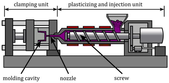
Figure 1.
Illustration of the basic structure of an injection molding machine.
The achievement of optimal injection molding results requires the careful coordination of a number of parameters, including those pertaining to the part properties, mold design, and material characteristics. This requires a process-oriented design approach, optimization of gating systems, and the establishment of appropriate speed profiles to ensure uniform filling of single and multiple cavities [11,12]. The injection molding process is inherently susceptible to significant inhomogeneities and often presents transient thermal or rheological behavior. For example, variations in mold thickness result in heterogeneous flow resistances [13]. Furthermore, the solidification of the melt’s boundary layers against the cooler mold wall induces local temporal changes in flow cross-sections, resulting in transient flow conditions [10].
Inhomogeneous filling conditions, which are characterized by varying flow velocities and shear stresses within the cavity, have an impact on the properties of the part, including the molecular chain orientations and the distribution of fillers. Such conditions can lead to typical processing defects, including geometric deformations such as shrinkage and warpage. Other phenomena that have been analyzed through injection molding simulation include weld lines, air traps, sink marks, surface defects, shrinkage voids, and burning [12]. A significant challenge is to achieve a balanced filling process, especially for complex geometries and multiple cavities. Consequently, numerical filling studies are of paramount importance during the early stages of product development and mold design, as they serve to identify and rectify potential design issues [10,14].
Subsequent validation of the mold can be conducted through systematic filling studies, which precisely reproduce the behavior of the injection mold under real conditions. This enables a direct comparison of the results with previously performed simulations, facilitating the identification and correction of potential inaccuracies in production that may have been undetected in the absence of simulations [10].
3. Numerical Modeling of the Filling Phase
3.1. Governing Equations
The filling phase employs a full volumetric approach, utilizing three-dimensional spatial discretization of the cavity. Both the cavity volume and the governing Navier-Stokes equations are discretized using the finite volume method (FVM), which has been established as standard for computational fluid dynamics (CFD) [6,9,15,16]. During the filling phase, the melt flow is assumed to be incompressible and, due to the relatively short process duration, isothermal [17]. Chang and Yang [17] demonstrated that isothermal models provide accurate and computationally efficient results for simulating the mold filling phase in injection molding, particularly when modeling three-dimensional isothermal flow of incompressible, highly viscous fluids. Furthermore, Shen [18] demonstrated that in thin-walled cavities, temperature differences within the polymer are negligible, confirming the accuracy of isothermal simplifications. The results showed that isothermal models are sufficient for characterizing the essential flow characteristics without introducing significant inaccuracies in the simulation. In Ansys CFX, the cavity filling can be modeled using either a homogeneous multiphase model or an inhomogeneous model. The homogeneous model assumes that both phases (air and polymer melt) are transported in the same ratio and share the same flow fields, such as velocity and temperature, allowing the transport equations to be combined [6,9]. Nevertheless, the findings of Igreja [19] demonstrate that the homogeneous model does not produce accurate results because the same boundary conditions are applied to both fluids. Haagh et al. [20,21] recommend the implementation of no-slip boundary conditions for the melt phase. The inhomogeneous model, as described by Mukras and Al-Mufadi [9], employs distinct flow fields for each phase, allowing the application of a free-slip boundary condition for the air phase. Interphase transfer terms are employed to regulate the interaction between phases. In addition, Baum et al. [10] describe a model incorporating a suitable rheological model for polymers, which enhances the accuracy of the simulation with Ansys CFX.
The following equations describe the two phases, designated as m and a, respectively (melt and air). The mass balance equation for each respective phase is as follows, as presented in [9,10,19,22]:
The aforementioned equation included time t, volume fraction r, density , velocity vector , and the dynamic viscosity . The momentum balance equation for each phase can be described by the following equation [9,10,19,22]:
It is assumed that the two phases fill the volume of the cavity completely. This condition is expressed as follows [9,10,19]:
In each phase, the terms and are related to the momentum caused by the gravitational force and are given by the following equations [9,19]:
As described in [9], the momentum balances include an interface that delimits the interphase interactions per unit volume. These interactions are characterized by the interphase momentum transfer terms and [10,19]. The relationship between these terms is defined as follows [9,10,19]:
As previously established by Igreja and Frank [19,22], it has been demonstrated that the interphase momentum transfer term, denoted here as , which incorporates both the drag coefficient and the interface length scale , can be described by the following equation:
3.2. Rheological Models
In the field of rheological modeling, the characterization of viscosity within a given material represents a crucial and fundamental objective. It has been observed that the viscosity of a polymeric melt can be substantially influenced by several variables, including the shear rate, temperature and pressure. It is also notable that thermoplastic polymers demonstrate pseudoplastic behavior at high shear rates [23]. The research conducted by Baum et al. [6] demonstrates the prevalence of various rheological models, many of which have applications in both the research and commercial sectors. It is notable that these models differ significantly in their mathematical approaches, which is of particular relevance in the context of injection molding simulation. An understanding of the rheological behavior of polymer melts is of significant importance for the accurate modeling and prediction of material flow.
3.2.1. Power-Law
One of the most frequently employed rheological models in the field of injection molding simulation is the Power-Law model, which posits a Power-Law relationship between the shear stress and shear rate of the polymer melt. The Power-Law model can be represented by the following mathematical formulation:
The parameters that are pertinent to this context are , which is defined as the Newtonian viscosity or the viscosity at zero shear rate, n is the Power-Law index, which takes on values between 0 and 1 for polymer melts and is the shear rate. When the viscosity at zero shear rate is equal to the constant fluid viscosity and the Power-Law index is equal to one, the resulting equation describes a Newtonian fluid [24,25].
3.2.2. Second-Order
The Second-Order model, developed by Moldflow, is aimed at enhancing the precision of viscosity estimations at low shear rates [24]. This model is mathematically formulated as follows [26]:
The equation presented herein encompasses material specific parameters A, B, C, D, E, and F, in addition to viscosity , shear rate , and temperature T.
3.2.3. Herschel-Bulkley
The Herschel-Bulkley model is a widely utilized non-Newtonian fluid model, particularly effective in characterizing fluids with a yield stress, such as Bingham fluids, which also display shear thinning behavior. This mathematical representation of the Herschel-Bulkley model is as follows [27,28]:
The Herschel–Bulkley model incorporates three key parameters: yield stress, consistency index, and flow index. The model is contingent upon the presence of a specific threshold stress . Below this threshold, the material behaves like a solid and can sustain stress without flow. Above the threshold, the material shows the characteristics of a Power-Law fluid. The value of n determines the fluid’s behavior: indicates shear thinning, indicates shear thickening and reduces the model to a Newtonian fluid behavior above the critical yield stress [28,29,30,31,32].
3.2.4. Carreau
The Carreau model is commonly employed to characterize the flow behavior of polymers. This model originated from the seminal works of Bird and Carreau [33,34], and further contributions by Yasuda et al. [35]. It can be described mathematically as follows:
The coefficients , , and each serve specific functions in characterizing the flow behavior of the material. Specifically, corresponds to zero viscosity, represents the transition region between Newtonian flow and structurally viscous behavior, and indicates the slope of the function within the structurally viscous region. It is important to note that all three coefficients are positive, with being less than 1 [36,37].
In their study, Menges et al. [38] adapted this model by incorporating the Williams-Landel-Ferry (WLF) temperature shift factor . This modification resulted in the Carreau-WLF model, whose equation is expressed as follows [39]:
The Williams-Landel-Ferry (WLF) equation, which was initially proposed by Williams [40] and subsequently refined by Ferry [41], provides the most accurate description of the temperature dependence of viscosity in amorphous thermoplastics at lower temperatures. This equation expresses the viscosity of the polymer at a given temperature relative to a reference viscosity, which is defined at a specified reference temperature.
The viscosity of the polymer is described in terms of its relative viscosity at a specific temperature T, in comparison to a reference viscosity at a reference temperature [30,42].
This equation applies to polymers only within the zero-shear viscosity range. The glass transition temperature is commonly used as the reference temperature , with constants and . As indicated in [40,43] is significantly lower than typical processing temperatures. In contrast to other proposed alternatives, van Krevelen [44] presents an alternative formulation for that is more suitable for the given context. The alternative formulation is expressed as , resulting in the values of and [45]. However, it is not typical to directly measure the viscosity of a polymer at the reference temperature . Instead, the measurement is conducted at a temperature within the processing temperature range . This necessitates the application of a secondary shift between the measurement or processing temperature and the reference temperature . The following equation represents the relationship between the viscosity at and the actual temperature T. [30,46]
The subsequent equation is composed of two distinct terms. The first term denotes the shift between the measurement temperature , and the reference temperature . The second term denotes the shift between the desired temperature T, and the reference temperature .
The approach proposed by Winter [47] is often employed in the denominator of Equation (14). This approach results in the term being commonly used [48,49,50,51]. This results in the approaches of the Carreau Winter model, as presented in Equation (18), and the Carreau-WLF Winter model, as described in Equation (19).
3.2.5. Bird-Carreau
The Bird–Carreau model represents a comprehensive mathematical framework for the characterization of the viscosity behavior of polymers as a function of shear rate [52,53]. The model is expressed in the following equation:
In this Equation, represents the viscosity at zero shear rate, denotes a characteristic time constant, is the shear rate, n represents the Power-Law index and is the infinite shear rate viscosity.
3.2.6. Cross
The Cross model accounts for the effects of shear rate and temperature on viscosity. It is comparable to the Carreau model and acquires both Newtonian and shear-thinning behavior [6]. The shear-thinning behavior is represented by the generalized Cross equation [54], which is a well-established alternative to the Bird–Carreau–Yasuda model [37]. The mathematical formulation of this model is expressed in the following equation [30].
The parameters utilized to characterize the rheological behavior of the fluid are the zero shear rate viscosity , the infinite shear rate viscosity , the time constant K, and the Power-Law index n. These parameters characterize the fluid’s shear thinning behavior. If the viscosity is negligible at infinite shear rate, the Cross model can be expressed in the following form [51].
Here, represented the critical shear stress at the transition from the Newtonian plateau. The defining characteristics include the Power-Law index n and the value .
The following equation can be employed for the purpose of determining the zero shear rate viscosity, with respect to the effects of temperature within the framework of the WLF approach [55,56,57]. This can be considered analogous to the temperature shift factor [55,56].
In this equation, represents the viscosity at the reference temperature , serves as a descriptor of the temperature, and serves as a descriptor of the polymer pressure dependence of the viscosity [5].
4. Modeling of the Filling Phase
For the purpose of this investigation, the same geometric configuration is employed in both the simulation and the experiments, cf. Figure 2. The mold filling simulation is configured and executed within the Ansys CFX framework. In this simulation, an inhomogeneous multiphase model [20] was employed to represent the filling process.
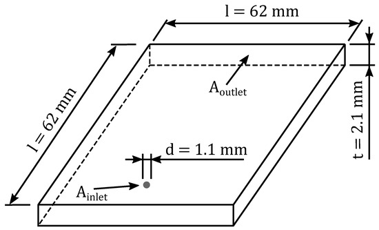
Figure 2.
Description of the geometric configuration.
The following boundary conditions are employed to reproduce the real process properties of the mold filling during injection molding, based on the research by Mukras and Al-Mufadi [9] and Baum et al. [10]. Two different boundary conditions are implemented to account for the complex interactions at the cavity wall boundaries. At the melt boundary, called the “melt wall” , a no-slip condition is imposed, characterized by a velocity vector . A free slip condition is imposed at the air boundary, called the “air wall” . This is represented mathematically by , where T is the stress tensor and n is the normal vector to the surface. The inlet surface, , is subjected to a constant mass flow rate of the melt, . In order to enhance computational efficiency, a symmetrical halved geometry is utilized. Furthermore, all variables are initialized with each prescribed initial boundary condition or appropriate estimated values [9].
The inlet conditions are specified with a constant mass flow rate of for the halved geometry. The outlet is configured as an opening and defined with a static pressure of . The inlet temperature is maintained at , while the wall temperature is fixed at . The CFD simulation in Ansys CFX employed a volumetric mesh comprising pyramids, tetrahedra, and wedges. The total number of elements in the model is 29,911. The mesh was prepared with five inflation layers at the walls and a maximum element size of . The simulation employs an adaptive time step control with a maximum time step of . For all equations, a residual convergence target of is employed, with a limit of 50 iterations.
The material properties of the air and the polymer PA66, designated as Schulamid 66 SK 1000 from LyondellBasell, are presented in Table 1 [10,14].

Table 1.
Overview of material properties of air and Schulamid 66 SK 1000 used for simulation.
The viscosity behavior of the rheological models was fitted based on data points extracted from the CAMPUS database. For this purpose, the nonlinear least-squares Levenberg-Marquardt (nlsLM) fitting algorithm was employed in the software R. In order to ascertain these data points, the viscosity values were considered in relation to the shear rate at three distinct temperatures. The data points are given in Table 2 [58].
Table 2.
Overview of the data points for the rheological properties of Schulamid 66 SK 1000.
The melt is conceptualized as a viscous fluid with a non-Newtonian, isothermal, and incompressible flow. The rheological properties of non-Newtonian fluids are described by several different mathematical models, including the Power-Law, Second-Order, Herschel-Bulkley, Carreau, Carreau-WLF, Carreau Winter, Carreau-WLF Winter, Bird-Carreau, Cross and Cross-WLF. Table 3 presents the parameters of the rheological models, as well as the coefficient of determination () and the Root Mean Square Error (RMSE) between rheological model and the data points of the CAMPUS database the determined parameters.
Table 3.
Overview of the parameters of the rheological models.
The evaluation of various rheological models based on their RMSE and values indicates significant differences in their predictive accuracy and quality of fit. The Second-Order model demonstrates the lowest RMSE (7.7517) and the highest value (0.9992), indicating superior predictive accuracy and an excellent fit to the data. Similarly, the Cross-WLF model also demonstrates good performance, with an RMSE of 8.217 and an value of 0.9991, establishing it as a leading model for predicting viscosity of polymer melts. Other models, including Herschel-Bulkley, Carreau, Carreau Winter, and Cross, also demonstrate good predictive accuracy, with RMSE values of approximately 80.7 and values of approximately 0.917. While these models are reliable, they do not show the same exceptional performance as the Second-Order and Cross-WLF models. In contrast, the Power-Law, Carreau-WLF Winter, and Bird-Carreau models exhibit higher RMSE values and lower values compared to the top-performing models, indicating less accuracy and fit.
Figure 3, Figure 4 and Figure 5 present the mathematical functions of the rheological models as a double-logarithmic plot for a specific temperature, with the viscosity as a function of the shear rate. It becomes evident that the Power-Law model can only approximate the viscosity curve to some extent due to its mathematical foundation and limitations. The remaining rheological models demonstrate a high degree of correlation with the RMSE and values presented in Table 3. Figure 3, Figure 4 and Figure 5 demonstrate that not all rheological models show an adequate representation of the temperature dependence, resulting in a greater discrepancy with the data points.
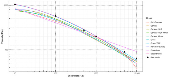
Figure 3.
Double-logarithmic plot of viscosity versus shear rate for the fitted rheological models and the data points of the CAMPUS database at a temperature of .
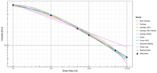
Figure 4.
Double-logarithmic plot of viscosity versus shear rate for the fitted rheological models and the data points of the CAMPUS database at a temperature of .
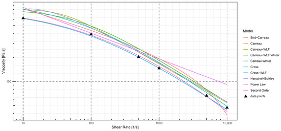
Figure 5.
Double-logarithmic plot of viscosity versus shear rate for the fitted rheological models and the data points of the CAMPUS database at a temperature of .
5. Experimental Design
The experimental design is based on the research of Baum et al. [10] on the flow behavior of the melt in an injection mold, which was conducted using various viscosity models. The focus of the experiments is the tracking of the flow front in the cavity. The experimental configuration involves a two-cavity mold for specimen production, with each cavity measuring in length and width and a thickness of . The experiments are conducted using an Engel EM 200/100 tie-bar-less all-electric injection molding machine, which has a screw diameter and a maximum clamping force of . In accordance with the simulation, the material Schulamid 66 SK 1000 from LyondellBasell will be employed in the experiments. Table 4 presents a summary of the material properties of the employed polymer [58].
Table 4.
Material properties Schulamid 66 SK 1000 used for experiments.
The injection molding experiments were employed to substantiate the results of the simulations. Initially, the parameters for the injection molding process were identified and established, as outlined in Table 5. Subsequently, a series of fills was conducted without holding pressure, starting with a metering volume set much lower than the required amount to fill the cavity and incrementally increasing it with each cycle. The parts ejected from the mold demonstrated the progression of the flow front [10]. This test involved two consecutive filling stages, allowing for detailed observation of the melt entering the cavity and progressing to full cavity filling.
Table 5.
Experimental set-up data for the injection molding machine Engel EM 200/100.
The influence of filling pressure causes the melt column to undergo compression between the screw tip and the flow front. After reaching the changeover point and stopping injection, this column decompresses, affecting the filling level achieved. As the simulation does not account for compressibility, it is crucial to maintain the melt column size constant to ensure accurate comparison with experimental results. Therefore, the filling series was conducted by adjusting the metering volume rather than altering the changeover point. This method ensures that the compressible melt column’s influence remains consistent across different filling levels, a factor that is not further analyzed in this study. All other parameters were maintained at their pre-determined values, and 10 initial cycles per set were performed to achieve a steady-state condition for the machine and mold [10]. After the experimental study, the molded parts were digitized for comparative evaluation against the simulation results. The components were positioned within the mold insert and photographed with the mold facing upwards, cf. Figure 6. In order to ensure a consistently optimal perspective for all images, a stationary camera was positioned above the mold insert. The point-shaped tunnel sprue ensures precise alignment of the molded parts within the mold cavity [10].
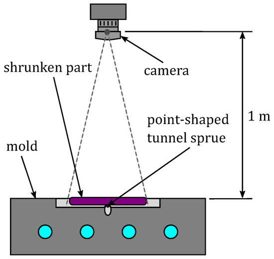
Figure 6.
Configuration for the digitization of molded parts.
After recording the filling levels, the images were first processed and scaled by the post-shrinkage of the parts. In this study, the volumetric homogeneous shrinkage was 1.95%. The shrunk parts no longer correspond to the dimensions of the actual filling level in the mold. Therefore, the complete filled part was initially utilized, and this was subsequently enlarged in both length and width in the image-processing stage until its dimensions corresponded entirely to those of the cavity. The scaling factors thus obtained were then applied similarly to the other images of the filling stages [10].
6. Evaluation of Simulation and Experimental Results
In order to compare the simulation results with the results of the experiments, the time steps and of the filling process were selected as representative examples. The images of the mold parts from the respective experiments at the indicated points in time are presented in Figure 7. The setup for digitizing molded parts was used to transfer the experimental flow front data into a two-dimensional coordinate system. The data extraction software DigitizeIt is employed to calculate the respective point data from digitized images and make it available for the specified two-dimensional coordinate system. This software is used to convert graphical information into digital information in the form of coordinate points [10,59,60].
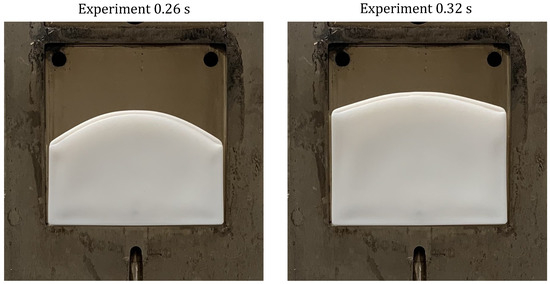
Figure 7.
Digitization of the molded parts at the time and .
In order to accurately and quantitatively compare the rheological models, the coordinates of the points characterizing the flow front in the mid-plane of the volume are extracted from Ansys CFX. The parabolic shape of the flow front in the thickness direction allows for the effective utilization of the outermost region of the flow front in the mid-plane for analytical purposes. The digitized data points of the experiments and the simulation of the rheological models at the time points under consideration are presented in Figure 8 and Figure 9.
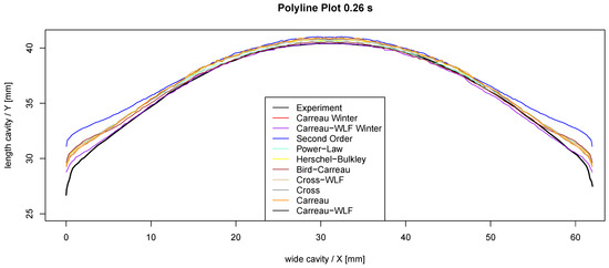
Figure 8.
Simulation and experimental results for the flow front at .
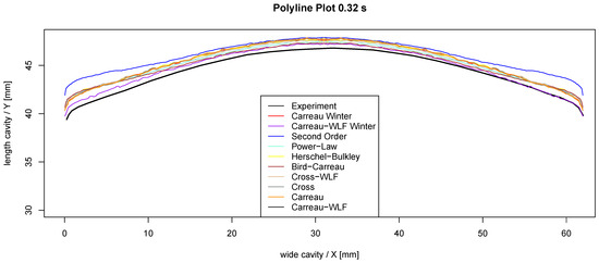
Figure 9.
Simulation and experimental results for the flow front at .
Figure 8 and Figure 9 demonstrate that the majority of rheological models reproduce the flow behavior in a similar manner. However, the Second-Order model shows a significant deviation in the edge region from the other rheological models and the experimental results. While the models are quite close to the experiments in the middle range of the flow front at the time step of , they are slightly ahead at the time step of . Both time steps demonstrate that the models approximate the experiments quite good in the middle of the flow front, while they run slightly further ahead in the edge region of the flow front. It is evident that the real flow front of the experiments is not perfectly symmetrical. This discrepancy can be attributed to minor asymmetries in the temperature distribution of the mold, surface roughness, and manufacturing tolerances. It is also pertinent to note that the Carreau-WLF Winter model has a better approximation of the wall region compared to the other models.
The Table 6 presents the results of the RMSE for various rheological models in comparison to the experimental data at two time steps. A lower RMSE value indicates a more accurate representation of the flow front. The Carreau-WLF Winter model shows the lowest RMSE values at both time steps, with values of 0.5751 at and 0.4192 at . This indicates that this model predicts the flow most accurately. The Carreau model also shows low RMSE values, 0.9563 at and 0.9763 at , providing reliable predictions. However, it is less accurate than the Carreau-WLF Winter model. The Power-Law model shows moderate performance, with RMSE values of 1.0978 at and 0.9258 at . While the model performs better than some existing models, it is not the most accurate solution. The Second-Order model shows the highest RMSE values, 2.0186 at and 1.8669 at , indicating the poorest model performance. This indicates that the model is less suitable for accurately predicting the flow. The Herschel-Bulkley model presents satisfactory performance, with RMSE values of 1.0606 at and 1.0125 at . However, it is not the most accurate model. The Cross and Cross-WLF models have moderate RMSE values. The Cross model shows values of 1.0948 at and 1.0122 at , while the Cross-WLF model performs better at (0.9018) but is not as good at (1.112). The Bird-Carreau model shows moderate performance, RMSE values of 1.1020 at and 0.9963 at . The values of the RMSE show a high comparison with the visual results presented in Figure 8 and Figure 9. It can be observed that the Second-Order model shows a significant deviation. However, the Carreau-WLF winter model represents the optimal approximation of the flow front. This can be attributed primarily to the more accurate representation of the edge region of the flow front.
Table 6.
RMSE between the rheological models and the experimental data at the time and .
Figure 10 presents the temperature distribution of various rheological models at the specified time points of and in the mid-plane. It is evident that the rheological models show disparate temperature influence characteristics. While the Power-Law, Second-Order, and Cross-WLF models demonstrate a pronounced temperature fluctuation within the filling volume, the other rheological models shows a markedly more homogeneous temperature distribution. All rheological models demonstrate a higher temperature in the edge region and in the region of the sprue.
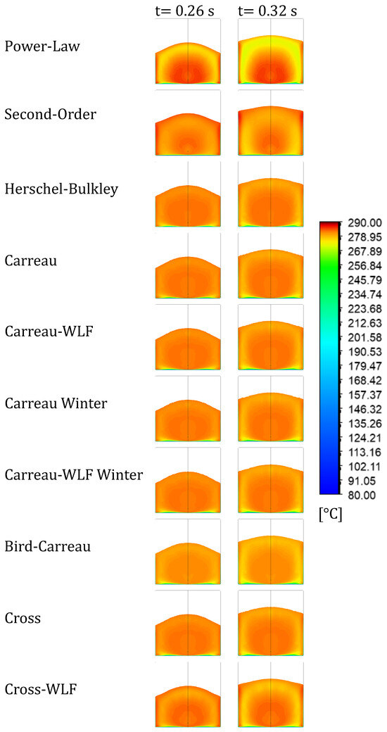
Figure 10.
Temperature distribution of the simulated rheological models in the mid-plane at and .
Figure 11 presents the distribution of the shear rate for the various rheological models. It can be observed that the shear rate for the Power-Law, Second-Order, and Cross-WLF models is more significant and more homogeneously distributed than for the other rheological models. In contrast, the shear rate for the Herschel-Bulkley, Carreau, Carreau-WLF, Carreau Winter, Carreau-WLF Winter, Bird-Carreau, and Cross models is more inhomogeneously distributed. In the wall region of the flow front and near the sprue, these models have a higher shear rate in the middle region of the filling volume.
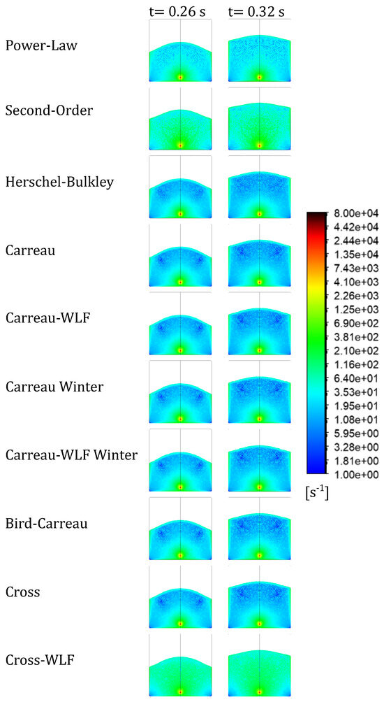
Figure 11.
Shear rate distribution of the simulated rheological models in the mid-plane at and .
Figure 12 presents the viscosity distributions of the rheological models. The characteristics of the viscosity distributions are different. The results demonstrate a clear correlation between shear rate and viscosity in all models. The Power-Law, Second-Order, Cross, and Cross-WLF models show a lower viscosity in the region close to the sprue and the middle region. In the wall region near the flow front, these rheological models show a lower viscosity. The Herschel-Bulkley and Bird-Carreau models show similar viscosity characteristics in the wall and near-sprue regions as the previous models. However, in the middle region of the filling volume, the Herschel-Bulkley model does show an average higher viscosity, with small low-viscosity spots, than the Bird-Carreau model. The Carreau, Carreau-WLF, Carreau Winter, and Carreau-WLF Winter models have a similar homogeneous viscosity in the middle region and the region close to the sprue. This viscosity is similarly low as in all other models. However, the wall region and that of the sprue are more clearly characterized by a low viscosity in the winter models.
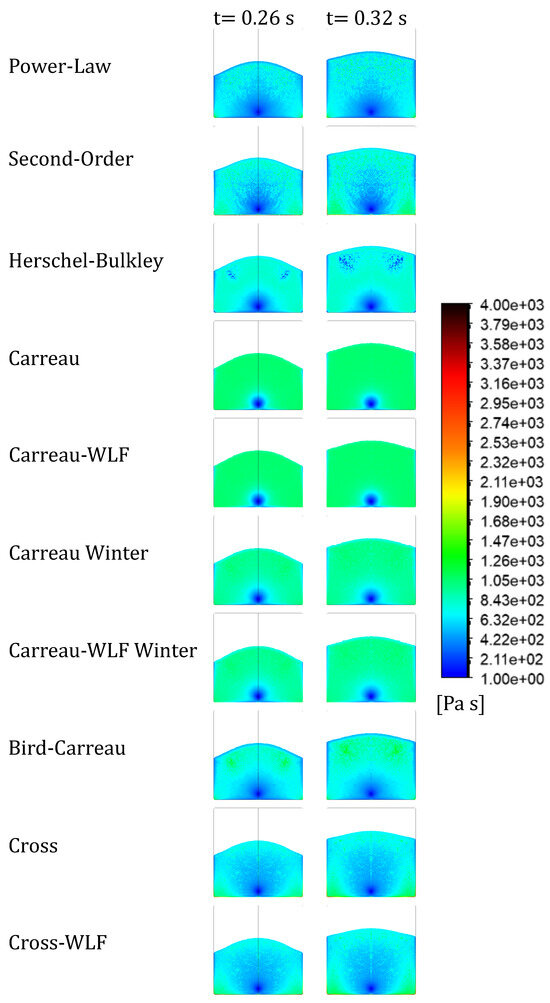
Figure 12.
Viscosity distribution of the simulated rheological models in the mid-plane at and .
In order to illustrate the influence of shear rate and temperature on viscosity in different rheological models, a comparison is made between the specific characteristics of each model in Table 7. The relationship between the influence on viscosity is demonstrated by comparing Figure 10, Figure 11 and Figure 12. The Power-Law model demonstrates a distinct correlation between viscosity and shear rate, with no temperature influence. This indicates that the viscosity in this model decreases with increasing shear rate, regardless of the temperature. In contrast, the Second-Order model demonstrates a sensitivity to changes in both shear rate and temperature. This model shows a decrease in viscosity with both increasing shear rate and increasing temperature. The Herschel-Bulkley model and the Carreau model appear similar to the Power-Law model in that they both demonstrate a strong dependence on the shear rate but no dependence on the temperature. The viscosity of these models decreases with increasing shear rate, but remains independent of temperature. The Carreau-WLF, Carreau-WLF Winter, and Cross-WLF models are notable for their dependence on both shear rate and temperature. In these models, it is observed that both an increase in the shear rate and an increase in temperature result in a decrease in viscosity. In contrast, the Carreau-Winter model demonstrates a dependence on the shear rate alone, with no temperature-related influence. Consequently, viscosity decreases as the shear rate increases, irrespective of the temperature. As with the other models, which are not temperature-dependent, the Bird-Carreau model and the Cross model also have a main reaction to the shear rate. In these models, viscosity is observed to decrease with increasing shear rate, independent of the temperature. It is evident that the viscosity of all rheological models depends on the shear rate. This implies that the viscosity of these models decreases with increasing shear rate. Only the Second-Order, Carreau-WLF, Carreau-WLF Winter, and Cross-WLF models in particular demonstrate a dependence on temperature, i.e., a decrease in viscosity with increasing temperature. These models offer a more differentiated adjustment of the viscosity under varying process conditions, while the other models, which only react to changes in the shear rate, remain less sensitive to temperature changes.
Table 7.
Overview of the rheological models and their influencing variables.
7. Conclusions and Outlook
The flow front contours in Figure 8 and Figure 9 show that most rheological models reproduce the flow behavior on a similar accuracy level. However, the Second-Order model differs significantly in the edge region of the flow front from the other models and the experimental results. While the rheological models in the middle region of the flow front come close to the experimental values at the time of , they are slightly ahead of the experiments at the time of . This shows that the rheological models approximate the experiments well in the middle region of the flow front, but run slightly ahead in the wall region. This effect results form the lack of modeling of the back pressure in the cavity and the associated -relationships. The real flow front of the experiments is not perfectly symmetrical, which is due to slight asymmetries in the temperature distribution of the mold, surface roughnesses and manufacturing tolerances. The Carreau-WLF Winter model shows the best approximation to the wall region compared to the other models. This observation confirms similar research findings that highlight the enhanced capability of the Carreau-WLF Winter model in modeling temperature-dependent viscosity effects during injection molding simulations [5,6]. The RMSE values presented in Table 6 confirm these observations. The Carreau-WLF Winter model provides the most accurate prediction of the flow, as indicated by the lowest RMSE values. The Carreau model and the Power-Law model follow with moderate RMSE values, while the Second-Order model has the highest RMSE values and thus the lowest accuracy. These RMSE values are in strong agreement with the visual results, which underlines the significant deviation in the edge region of the Second-Order model and the optimal approximation of the Carreau-WLF Winter model.
The analysis of the variables that influence viscosity indicates that all models are dependent on shear rate. This implies that viscosity decreases as shear rate increases. In addition, the Second-Order, Carreau-WLF, Carreau-WLF Winter, and Cross-WLF models exhibit a temperature-dependent viscosity, whereby the viscosity decreases with increasing temperature. The models allow for a differentiated adjustment of the viscosity under varying process conditions, whereas the other models remain less sensitive to temperature changes. Although all models demonstrate a comprehensible viscosity distribution influenced by the shear rate and temperature, there are slight differences in the middle region. The viscosity in the wall and sprue region is less than that observed in the middle region. However, the middle region shows notable differences. While the Carreau models depict a relatively homogeneous viscosity distribution, the middle region shows a significantly more heterogeneous viscosity distribution in the other rheological models. The real viscosity cannot be definitively determined at this point. This would require the development of innovative measurement techniques that can accurately quantify viscosity within the cavity.
All rheological models demonstrate a comparable characteristic of the flow front, which indicates that the shear rate is the dominant factor in this context. The viscosity versus shear rate in Figure 3, Figure 4 and Figure 5 and the mathematical approximations of the rheological models do not directly indicate this context. Due to the linear representation of the Power-Law model in the double-logarithmic diagram, there is a potential for the model to be incorrectly interpreted as demonstrating a significantly worse filling behavior. Figure 10 presents the shear rate range, which demonstrates that the Power-Law model is in close alignment with the data points within the designated shear rate range. However, the results indicate that this is not the case. In conclusion, models that consider both shear rate and temperature offer the most accurate predictions for flow behavior and viscosity, demonstrating their superiority in modeling the filling phase of injection molding simulation. It is important to note that, while mathematical modeling of viscosity characteristics is a fundamental aspect, it is not a standalone solution. Furthermore, it is crucial to experimentally validate the effects of the polymer on the flow behavior. However, the results of this study are valid for the considered the geometry and polymer PA66. Although the results may serve as a reference for other polymers and more complex geometries, further research is required to thoroughly explore these aspects.
The obtained results show the potential for several promising research and development directions. It is also of great importance to pursue further refinement of the rheological models, particularly by incorporating additional influencing variables, such as pressure and specific material properties, with the aim of enhancing the precision of the predictions. The Carreau-WLF Winter model demonstrated the most accurate predictions of the flow front for PA66, suggesting that a detailed investigation and optimization of this model could provide new insights and potentially more effective modification possibilities. An alternative approach could be the development of hybrid models that combine the strengths of different models in order to achieve an even more accurate representation of flow behavior and viscosity under varying process conditions. Furthermore, the investigation and implementation of machine learning techniques and data-driven approaches to modeling and prediction could also open up new possibilities and improve the flexibility and accuracy of the rheological models. In the long term, the models developed should be integrated into industrial practice and their applicability tested in real production settings. This process includes the validation and adaptation of the models in a variety of industrial contexts, as well as the development of user-friendly software tools that facilitate the advanced modeling techniques accessibility to engineers and researchers. The combination of enhanced rheological models, advanced data acquisition techniques, and contemporary analysis and optimization methods presents a promising potentials for future research and development in the field of material processing and polymer flow modeling.
Author Contributions
Conceptualization, M.B.; methodology, M.B.; software, M.B.; validation, M.B., D.A. and T.R.; formal analysis, M.B., D.A. and T.R.; investigation, M.B.; resources, M.B.; data curation, M.B.; writing—original draft preparation, M.B.; writing—review and editing, M.B., D.A. and T.R.; visualization, M.B.; supervision, M.B., D.A. and T.R.; project administration, M.B.; funding acquisition, M.B. and D.A. All authors have read and agreed to the published version of the manuscript.
Funding
This research received no external funding.
Institutional Review Board Statement
Not applicable.
Informed Consent Statement
Not applicable.
Data Availability Statement
Data supporting this study are included within the article.
Conflicts of Interest
The authors declare no conflicts of interest.
References
- Li, B.; Wei, S.; Xuan, H.; Xue, Y.; Yuan, H. Tailoring fineness and content of nylon–6 nanofibers for reinforcing optically transparent poly(methyl methacrylate) composites. Polym. Compos. 2021, 42, 3243–3252. [Google Scholar] [CrossRef]
- Sim, K.; Gao, Y.; Chen, Z.; Song, J.; Yu, C. Nylon Fabric Enabled Tough and Flaw Insensitive Stretchable Electronics. Adv. Mater. Technol. 2019, 4, 1800466. [Google Scholar] [CrossRef]
- Li, J.; Yi, Y.; Wang, C.; Lu, W.; Liao, M.; Jing, X.; Wang, W. An Intrinsically Transparent Polyamide Film with Superior Toughness and Great Optical Performance. Polymers 2024, 16, 599. [Google Scholar] [CrossRef] [PubMed]
- Tutar, M.; Karakus, A. Numerical study of polymer melt flow in a three-dimensional sudden expansion: Viscous dissipation effects. J. Polym. Eng. 2014, 34, 755–764. [Google Scholar] [CrossRef]
- de Miranda, D.A.; Rauber, W.K.; Vaz Júnior, M.; Nogueira, A.L.; Bom, R.P.; Zdanski, P.S.B. Evaluation of the Predictive Capacity of Viscosity Models in Polymer Melt Filling Simulations. J. Mater. Eng. Perform. 2022, 32, 1707–1720. [Google Scholar] [CrossRef]
- Baum, M.; Anders, D.; Reinicke, T. Approaches for Numerical Modeling and Simulation of the Filling Phase in Injection Molding: A Review. Polymers 2023, 15, 4220. [Google Scholar] [CrossRef]
- Wilczyński, K.; Narowski, P. Simulation Studies on the Effect of Material Characteristics and Runners Layout Geometry on the Filling Imbalance in Geometrically Balanced Injection Molds. Polymers 2019, 11, 639. [Google Scholar] [CrossRef]
- Bakrani Balani, S.; Mokhtarian, H.; Coatanéa, E.; Chabert, F.; Nassiet, V.; Cantarel, A. Integrated modeling of heat transfer, shear rate, and viscosity for simulation-based characterization of polymer coalescence during material extrusion. J. Manuf. Process. 2023, 90, 443–459. [Google Scholar] [CrossRef]
- Mukras, S.M.S.; Al-Mufadi, F.A. Simulation of HDPE Mold Filling in the Injection Molding Process with Comparison to Experiments. Arab. J. Sci. Eng. 2016, 41, 1847–1856. [Google Scholar] [CrossRef]
- Baum, M.; Jasser, F.; Stricker, M.; Anders, D.; Lake, S. Numerical simulation of the mold filling process and its experimental validation. Int. J. Adv. Manuf. Technol. 2022, 120, 3065–3076. [Google Scholar] [CrossRef]
- Ding, Y.; Hassan, M.H.; Bakker, O.; Hinduja, S.; Bártolo, P. A Review on Microcellular Injection Moulding. Materials 2021, 14, 4209. [Google Scholar] [CrossRef] [PubMed]
- Zhou, H. Computer Modeling for Injection Molding: Simulation, Optimization, and Control; Wiley: Hoboken, NJ, USA, 2013. [Google Scholar] [CrossRef]
- Bociaga, E.; Jaruga, T. Visualization of melt flow lines in injection moulding. J. Achiev. Mater. Manuf. Eng. 2006, 18, 331–334. [Google Scholar]
- Baum, M.; Anders, D. A numerical simulation study of mold filling in the injection molding process. Comput. Methods Mater. Sci. 2021, 21, 25–34. [Google Scholar] [CrossRef]
- Anders, D.; Baum, M.; Alken, J. A Comparative Study of Numerical Simulation Strategies in Injection Molding. In Proceedings of the 14th WCCM-ECCOMAS Congress, Virtual, 11–15 January 2021. [Google Scholar] [CrossRef]
- Rusdi, M.S.; Abdullah, M.Z.; Mahmud, A.S.; Khor, C.Y.; Abdul Aziz, M.S.; Abdullah, M.K.; Yusoff, H.; Firdaus, S.M. Numerical Investigation on the Effect of Injection Pressure on Melt Front Pressure and Velocity Drop. Appl. Mech. Mater. 2015, 786, 210–214. [Google Scholar] [CrossRef]
- Chang, R.Y.; Yang, W.h. Numerical simulation of mold filling in injection molding using a three-dimensional finite volume approach. Int. J. Numer. Methods Fluids 2001, 37, 125–148. [Google Scholar] [CrossRef]
- Shen, S.F. Simulation of polymeric flows in the injection moulding process. Int. J. Numer. Methods Fluids 1984, 4, 171–183. [Google Scholar] [CrossRef]
- Igreja, R. Numerical Simulation of the Filling and Curing Stages in Reaction Injection Moulding, Using CFX. Ph.D. Thesis, Universidade de Aveiro, Aveiro, Portugal, 2007. [Google Scholar] [CrossRef]
- Haagh, G.A.A.V.; van de Vosse, F.N. Simulation of three-dimensional polymer mould filling processes using a pseudo-concentration method. Int. J. Numer. Methods Fluids 1998, 28, 1355–1369. [Google Scholar] [CrossRef]
- Haagh, G.A.A.V.; Peters, G.W.M.; van de Vosse, F.N.; Meijer, H.E.H. A 3-D finite element model for gas-assisted injection molding: Simulations and experiments. Polym. Eng. Sci. 2001, 41, 449–465. [Google Scholar] [CrossRef]
- Frank, T. Advances in Computational Fluid Dynamics (CFD) of 3-dimensional gasliquid multiphase flows. In NAFEMS Seminar: Simulation of Complex Flows (CFD)—Applications and Trends; NAFEMS: Wiesbaden, Germany, 2005; pp. 1–18. Available online: https://www.researchgate.net/profile/Thomas-Frank-9/publication/291026181_Advances_in_computational_fluid_dynamics_CFD_of_3-dimensional_gas-liquid_multiphase_flows/links/5aacd9c7458515ecebe65a3e/Advances-in-computational-fluid-dynamics-CFD-of-3-dimensional-gas-liquid-multiphase-flows.pdf (accessed on 10 June 2024).
- Ahmad, Z.; Abdullah, M.K.; Ali, M.Z.; Md Zawawi, M.A. Electronic packaging and thermal management. In Polymers in Electronics; Elsevier: Amsterdam, The Netherlands, 2023; pp. 389–427. [Google Scholar] [CrossRef]
- Koszkul, J.; Nabialek, J. Viscosity models in simulation of the filling stage of the injection molding process. J. Mater. Process. Technol. 2004, 157–158, 183–187. [Google Scholar] [CrossRef]
- Mavridis, H.; Hrymak, A.N.; Vlachopoulos, J. Finite element simulation of fountain flow in injection molding. Polym. Eng. Sci. 1986, 26, 449–454. [Google Scholar] [CrossRef]
- Wang, W.; Li, X.; Han, X. Numerical simulation and experimental verification of the filling stage in injection molding. Polym. Eng. Sci. 2012, 52, 42–51. [Google Scholar] [CrossRef]
- Herschel, W.H.; Bulkley, R. Konsistenzmessungen von Gummi-Benzollösungen. Kolloid-Zeitschrift 1926, 39, 291–300. [Google Scholar] [CrossRef]
- Valencia, A.; Morales, H.; Rivera, R.; Bravo, E.; Galvez, M. Blood flow dynamics in patient-specific cerebral aneurysm models: The relationship between wall shear stress and aneurysm area index. Med. Eng. Phys. 2008, 30, 329–340. [Google Scholar] [CrossRef] [PubMed]
- Tosello, G.; Marhöfer, D.M.; Islam, A.; Müller, T.; Plewa, K.; Piotter, V. Comprehensive characterization and material modeling for ceramic injection molding simulation performance validations. Int. J. Adv. Manuf. Technol. 2019, 102, 225–240. [Google Scholar] [CrossRef]
- Osswald, T.A.; Rudolph, N. Polymer Rheology: Fundamentals and Applications; Hanser eLibrary, Hanser: Munich, Germany, 2014. [Google Scholar] [CrossRef]
- Kutsbakh, A.A.; Muranov, A.N.; Semenov, A.B.; Semenov, B.I. The Rheological Behavior of Powder–Polymer Blends and Model Description of Feedstock Viscosity for Numerical Simulation of the Injection Molding Process. Polym. Sci. Ser. D 2022, 15, 701–708. [Google Scholar] [CrossRef]
- Rudert, A.; Schwarze, R. Numerical simulation of the filling behavior of a Non-Newtonian Fluid. Proc. Appl. Math. Mech. 2006, 6, 585–586. [Google Scholar] [CrossRef]
- Bird, R.B.; Carreau, P.J. A nonlinear viscoelastic model for polymer solutions and melts—I. Chem. Eng. Sci. 1968, 23, 427–434. [Google Scholar] [CrossRef]
- Carreau, P.J. Rheological Equations from Molecular Network Theories. Trans. Soc. Rheol. 1972, 16, 99–127. [Google Scholar] [CrossRef]
- Yasuda, K.; Armstrong, R.C.; Cohen, R.E. Shear flow properties of concentrated solutions of linear and star branched polystyrenes. Rheol. Acta 1981, 20, 163–178. [Google Scholar] [CrossRef]
- Geiger, K.; Khnle, H. Analytische Berechnung einfacher scherstrmungen aufgrund eines fliegesetzes vom carreauschen typ. Rheol. Acta 1984, 23, 355–367. [Google Scholar] [CrossRef]
- Hieber, C.A.; Chiang, H.H. Shear-rate-dependence modeling of polymer melt viscosity. Polym. Eng. Sci. 1992, 32, 931–938. [Google Scholar] [CrossRef]
- Menges, G.; Wortberg, J.; Michaeli, W. Estimating the Viscosity Function via the Melt Flow Index. Kunstst Ger Plast 1978, 68, 47–50. [Google Scholar]
- Karrenberg, G. CFD-Simulation der Kunststoffplastifizierung in einem Extruder mit durchgehend genutetem Zylinder und Barriereschnecke. Z. Kunststofftechnik 2016, 1, 205–238. [Google Scholar] [CrossRef]
- Williams, M.L.; Landel, R.F.; Ferry, J.D. The Temperature Dependence of Relaxation Mechanisms in Amorphous Polymers and Other Glass-forming Liquids. J. Am. Chem. Soc. 1955, 77, 3701–3707. [Google Scholar] [CrossRef]
- Ferry, J.D. Viscoelastic Properties of Polymers, 3rd ed.; John Wiley & Sons: New York, NY, USA; Chichester, UK; Brisbane, Australia; Toronto, ON, Canada; Singapore, 1980. [Google Scholar]
- Laun, H.M. Description of the non-linear shear behaviour of a low density polyethylene melt by means of an experimentally determined strain dependent memory function. Rheol. Acta 1978, 17, 1–15. [Google Scholar] [CrossRef]
- Angell, C.A. Why C1 = 16–17 in the WLF equation is physical—And the fragility of polymers. Polymer 1997, 38, 6261–6266. [Google Scholar] [CrossRef]
- van Krevelen, D.W. Properties of Polymers, 2nd ed.; Elsevier: Amsterdam, The Netherlands, 1976. [Google Scholar]
- Rowland, H.D.; King, W.P.; Sun, A.C.; Schunk, P.R.; Cross, G.L.W. Predicting Polymer Flow during High-Temperature Atomic Force Microscope Nanoindentation. Macromolecules 2007, 40, 8096–8103. [Google Scholar] [CrossRef]
- Fan, B.; Kazmer, D.O. Low-temperature modeling of the time-temperature shift factor for polycarbonate. Adv. Polym. Technol. 2005, 24, 278–287. [Google Scholar] [CrossRef]
- Winter, H.H. Temperature-induced pressure gradient in the clearance between screw flight and barrel of a single screw extruder. Polym. Eng. Sci. 1980, 20, 406–412. [Google Scholar] [CrossRef]
- Schroeder, T. Rheologie der Kunststoffe: Theorie und Praxis; Hanser: Munich, Germany, 2018. [Google Scholar]
- Ilinca, F.; Hétu, J.F. Three-dimensional simulation of multi-material injection molding: Application to gas-assisted and co-injection molding. Polym. Eng. Sci. 2003, 43, 1415–1427. [Google Scholar] [CrossRef]
- Kamal, M.R.; Isayev, A.I.; Liu, S.J.; White, J.L. (Eds.) Injection Molding: Technology and Fundamentals; Progress in Polymer Processing; Hanser: Munich, Germany, 2009. [Google Scholar]
- Yavari, R.; Khorsand, H.; Sardarian, M. Simulation and modeling of macro and micro components produced by powder injection molding: A review. Polyolefins J. 2020, 7, 45–60. [Google Scholar] [CrossRef]
- Buchmann, M.; Theriault, R.; Osswald, T.A. Polymer flow length simulation during injection mold filling. Polym. Eng. Sci. 1997, 37, 667–671. [Google Scholar] [CrossRef]
- Domurath, J.; Saphiannikova, M.; Férec, J.; Ausias, G.; Heinrich, G. Stress and strain amplification in a dilute suspension of spherical particles based on a Bird–Carreau model. J. Non-Newton. Fluid Mech. 2015, 221, 95–102. [Google Scholar] [CrossRef]
- Cross, M.M. Rheology of non-Newtonian fluids: A new flow equation for pseudoplastic systems. J. Colloid Sci. 1965, 20, 417–437. [Google Scholar] [CrossRef]
- Shi, X.Z.; Huang, M.; Zhao, Z.F.; Shen, C.Y. Nonlinear Fitting Technology of 7-Parameter Cross-WLF Viscosity Model. Manuf. Process. Technol. 2011, 189–193, 2103–2106. [Google Scholar] [CrossRef]
- Mishra, A.A.; Momin, A.; Strano, M.; Rane, K. Implementation of viscosity and density models for improved numerical analysis of melt flow dynamics in the nozzle during extrusion-based additive manufacturing. Prog. Addit. Manuf. 2022, 7, 41–54. [Google Scholar] [CrossRef]
- Zhu, H.Y.; Xiao, X.T.; Zhang, Z.H. Fitting and Verification Viscosity Parameter of ABS/Aluminum Blends. Manuf. Process. Technol. 2011, 308–310, 824–830. [Google Scholar] [CrossRef]
- M-Base Engineering + Software GmbH. CAMPUSplastics|Datenblatt SCHULAMID® 66 SK 1000. Available online: https://www.campusplastics.com/material/pdf/141558/SCHULAMID66SK1000?sLg=de (accessed on 10 June 2024).
- Phan, K.; Tian, D.H.; Cao, C.; Black, D.; Yan, T.D. Systematic review and meta-analysis: Techniques and a guide for the academic surgeon. Ann. Cardiothorac. Surg. 2005, 4, 112–122. [Google Scholar] [CrossRef]
- Atkinson, G. Shear rate normalization is not essential for removing the dependency of flow-mediated dilation on baseline artery diameter: Past research revisited. Physiol. Meas. 2014, 35, 1825–1835. [Google Scholar] [CrossRef]


Disclaimer/Publisher’s Note: The statements, opinions and data contained in all publications are solely those of the individual author(s) and contributor(s) and not of MDPI and/or the editor(s). MDPI and/or the editor(s) disclaim responsibility for any injury to people or property resulting from any ideas, methods, instructions or products referred to in the content. |
© 2024 by the authors. Licensee MDPI, Basel, Switzerland. This article is an open access article distributed under the terms and conditions of the Creative Commons Attribution (CC BY) license (https://creativecommons.org/licenses/by/4.0/).