Abstract
Optimizing energy consumption is an important aspect of industrial competitiveness, as it directly impacts operational efficiency, cost reduction, and sustainability goals. In this context, anomaly detection (AD) becomes a valuable methodology, as it supports maintenance activities in the manufacturing sector, allowing for early intervention to prevent energy waste and maintain optimal performance. Here, an AD-based method is proposed and studied to support energy-saving predictive maintenance of production lines using time series acquired directly from the field. This paper proposes a deep echo state network (DeepESN)-based method for anomaly detection by analyzing energy consumption data sets from production lines. Compared with traditional prediction methods, such as recurrent neural networks with long short-term memory (LSTM), although both models show similar time series trends, the DeepESN-based method studied here appears to have some advantages, such as timelier error detection and higher prediction accuracy. In addition, the DeepESN-based method has been shown to be more accurate in predicting the occurrence of failure. The proposed solution has been extensively tested in a real-world pilot case consisting of an automated metal filter production line equipped with industrial smart meters to acquire energy data during production phases; the time series, composed of 88 variables associated with energy parameters, was then processed using the techniques introduced earlier. The results show that our method enables earlier error detection and achieves higher prediction accuracy when running on an edge device.
1. Introduction
In recent years, the relationship between industrial production activities and climate change has become increasingly evident; greenhouse gas (GHG) emissions have been highlighted in United Nations climate change conferences [1] as particularly worrying, with the goal of improving the efficiency of industrial production and manufacturing systems by reducing global emissions by by 2030. Industrial processes are one of the pillars of the world economy, but it is important that they evolve through the use of more sustainable designs of production plants with the aim of reducing their environmental impact in terms of pollution and using resources more efficiently. In this context, in order to optimize energy costs, reduce waste, and improve environmental management, one of the crucial aspects for the industrial sector is energy management. For this reason, the analysis of production performance both in terms of efficiency and in terms of consumption has increasingly attracted attention [2,3]. Energy saving can be achieved in different ways, for example, through the application of energy-efficient technologies in production areas, operational planning improvement, and effective maintenance of all actors located in the factory. Indeed, in order to ensure the energy optimization of machinery and processes, both scheduled and predictive maintenance become essential. To ensure that a plant achieves the desired performance, it is important to design a monitoring system to gather information about the performance on maintenance operations and maintenance results. Usually, in a production plant, not only do normal wear and deterioration occur—which can often be detected by diagnostic techniques based on models, signals, or data, such as those reported in [4,5,6]—but other anomalies may also result from less easily diagnosed or measurable phenomena, especially if caused by manual operating errors, incorrect settings, or when the systems are pushed beyond their design limits. As a result, problems with production inefficiency, energy losses, increased costs, equipment downtime, plant unavailability, and excessive environmental pollution can eventually arise [7].
The effects of correct process design and operational maintenance on energy consumption have been addressed, for example, in energy-intensive sectors such as the steel industry [8] as well as in the study of the selection and diagnosis of cutting tools [9,10], optimizing the performance of machine parameters [11,12], and even preservation strategies for air pressure systems [13]. Further approaches used to account for inefficiencies are based on performance indicators, e.g., Miguel Calvo et al. [14] introduced overall environmental equipment effectiveness (OEEE), which allows one to take into account energy efficiency and sustainability when evaluating the effectiveness of the production processes, while in [15], a new performance indicator is proposed that also takes labor’s effectiveness into account. Regarding maintenance improvement, many different policies for industrial maintenance are available, but one of the most promising is predictive maintenance (PdM), which is generally defined as the use of prediction techniques and tools to estimate the remaining useful life (RUL) of a device or machinery, i.e., when repairs and corrections are needed in order for the production machinery to continue functioning properly [16]. Instead, Ref. [17] proposed a risk-based predictive maintenance approach for multi-state production systems, using mission reliability as the primary criterion considering three types of operational risks—fundamental, explicit, and implicit—to optimize maintenance strategies and minimize overall production costs. Several older approaches used to identify linear relationships in time series are based on statistical methods. Some of them are the autoregressive integrated moving average (ARIMA) [18], a prediction method based on past observations which differs in ensuring stationarity and residuals; seasonal ARIMA (SARIMA) [19], which allows one to include seasonal components; and Seasonal ARIMA with exogenous variables (SARIMAX) [20], which allows one to incorporate exogenous variables that exert influence over the series, thus enabling the modeling of external factors for more precise forecasts. Some noteworthy approaches are based on machine learning (ML) techniques to estimate the time remaining before a production line no longer functions properly [21,22]. Although this may sound attractive, it requires the availability of labeled or experimental data and complex mathematical or logical models, which makes their practical implementation difficult [23]. A further, often effective, approach is anomaly detection (AD). It not only focuses on predicting RUL, but it is based on detecting the first signs of a malfunction, or an anomaly, based on the analysis of time series collected from the machinery, which could indicate an impending failure. It can be used to discover interesting and unusual patterns and events [24]. However, most of the literature on the subject focuses mainly on the maintenance of power generation systems, such as wind farms [25,26,27], ocean wave farms [28], and so on, in order to improve their performances [29]. Although time series are widely used for AD purposes on production lines, to the authors’ knowledge, an AD method using DeepESN to support energy-saving maintenance for production lines by acquiring data directly from the field has not yet been investigated. Only a few works analyze online data streaming [30,31,32]. Furthermore, parts of the literature try to model complex system dynamic behaviors [33,34], requiring additional computational resources. The vehicle sector could also benefit from AD related to energy consumption, but their physical modeling is still very complex, e.g., Refs. [35,36], and poses serious limitations to traditional techniques, which could alternatively be addressed with new approaches based on data, as, for example, has been done for other equally complex systems such as robots [37]. Finally, there are still few ML solutions that can be trained and tested at the edge, i.e., on an embedded devices or on devices close to the data source, enabling processing at higher speeds and volumes [38] and in real time [39].
In this context, this paper proposes a method based on DeepESN for anomaly prediction in non-linear dynamical systems. Compared with traditional prediction methods such as the long short-term memory (LSTM) and recurrent neural networks (RNN), although both models show a similar trend in the time-series, the DeepESN-based method presents timelier error detection and achieves a higher prediction accuracy. Furthermore, the time-series prediction made by the DeepESN-based method proved to be more accurate, with the ability to predict the occurrence of a fault as clearly as the LSTM. In particular, by incorporating DeepESN into the developed AD algorithm, the temporal features of the time series data are extracted in order to predict the occurrence of an anomaly. In short, the main contributions of this work can be summarized as follows:
- Industrial solution proposal:A modular and commercial IIoT architecture is proposed which combines a Seneca S406 Smart Meter and an embedded device to ensure the repeatability of our solution across all available production lines in a factory scenario and the low latency requirements of future smart manufacturing systems. Specifically, the embedded device at the edge collects information from the IIoT module connected to the production line using the Modbus-TCP/IP protocol and considers all the energy parameters needed to apply the fault detection method.
- Anomaly detection modeling:The anomaly prediction problem is identified, experiments are carried out on a nonlinear dynamic system, and a DeepESN-based AD method is proposed to solve the prediction problem.
- Running at the Edge: Due to the limitations of the computational resources available in industrial plants, a model is proposed that can be trained and tested on devices embedded at the edge. The scheme proposes a deep network based on ESN units which captures complex temporal influences and requires low computational resources.
- Results and evaluations:Extensive experiments are conducted in a real scenario to evaluate the performance of the proposed method. The dataset contains the time series values of the 88 variables, which are associated with energy parameters acquired using the industrial smart meter and IIoT sensors already available on the market in order to promote the replication our experiments. The results show that our method presents timelier error detection and achieves a higher prediction accuracy.
The remainder of the article is organized as follows: Section 2 shows the works related to machine learning techniques used in the context of anomaly detection with a focus on those used for forecasting outcomes and requiring a few hardware resources. Section 3 describes preliminaries in introducing the two main architectures used for our purposes: ESN and LSTM. The proposed novel DeepESP-based anomaly detection method is introduced in Section 4, while Section 5 presents materials and methods describing the whole architecture from a hardware and software point of view. The experimental analysis, visualization of results, and discussion comparing different techniques are highlighted in Section 7. Finally, the last Section 8 points out the conclusions and future developments.
2. Related Work
Different ML techniques can be applied for AD, and the most significant can be summarized as follows:
- Recurrent Neural Network (RNN):This is an artificial neural network (ANN) that recognizes patterns in sequences of data such as those from sensors [40]. As an example, in [41], the authors proposed OC4Seq, a multi-scale one-class RNN used to capture different levels of sequential patterns simultaneously and to embed the discrete event sequences into latent spaces, where anomalies can be detected.
- Autoencoder Neural Networks (AE):These are a specific type of neural network that belongs to the class of generative models used in unsupervised learning. AEs are designed to efficiently compress input data into a lower-dimensional representation and then use that compressed information to reconstruct the original input. This process involves two main components: the encoder, which compresses the input data, and the decoder, which reconstructs the data from its compressed form. AEs are widely used for tasks such as dimensionality reduction, image denoising, and feature learning, improving the ability to capture the essential features of input data while eliminating noise and redundancy. The goal is to ensure that its latent space has good properties, which allows for the generation of new data [42].An unsupervised AD approach is proposed in [43] where the authors introduce a sliding-window convolutional variational autoencoder (SWCVAE) which can automatically learn normal patterns from time series data in training and can detect AD in real time, both spatially and temporally, by dealing with multivariate time series data. In [44], to improve the identification of values within a dataset that vary greatly from the others, the outliers, the authors propose using stacked autoencoders to extract features and then an ensemble of probabilistic neural networks to conduct majority voting and find outliers.
- Generative Adversarial Network (GAN):Deep adversarial neural networks are composed of two networks competing with each other. This setup creates a challenging adversary for the model, namely a discriminative network that learns to discern whether a sample originates from the distribution of false data or from the model. In this particular class of algorithms, the training consists of only ordinary data. Anything that is not classified in this way is labeled as an anomaly [45]. A conditional GAN was proposed in [46], and it jointly learns the generation of high-dimensional image space and the inference of latent space. This model consists of two encoders, a decoder, and a discriminator. Bidirectional GAN (BiGAN) was developed in [47], and it learns an encoder E which simultaneously maps input samples x to a latent representation z. This avoids the computationally expensive step of recovering a latent representation at test time. BiGANs was proposed in [48] to learn this inverse mapping produce a feature representation. In addition to the GAN framework, an encoder was used to map data to a latent representation.
AD is usually a difficult problem to solve. Most of the techniques in the literature are designed to address a specific application case of the general problem, e.g., related to the type of data input or model, the availability of labels for the training and testing data, or the types of anomalies. Furthermore, most of them require high computational efforts or resources and are too complex to be applied on different production lines. For these reasons, the focus of our work is on the DeepESN model as an alternative RNN model.
3. Preliminaries
This section presents an overview of the fundamental architectures underlying the DeepESN and LSTM models. The basic concepts of ESN are presented in Section 3.1, while those of LSTM are presented in Section 3.2. Finally, in Section 3.2.1, the efficiency of the long short-term memory model is discussed.
3.1. Fundamental Concepts of the Echo State Network
The ESN [49] is a particular RNN [50] model whose name comes from the concept that the historical encoding of the past (hidden state) is “echoed” in the future summed to the current time step. The ESN is a model of the reservoir computing framework [51] that collects extremely efficient recurrent neural network models.
3.1.1. Reservoir Computing
Reservoir computing models are characterized by an architecture divided into a reservoir and a readout. The reservoir represents the recurrent part that allows for encoding the temporal dependencies of time series and maps them into a vector with higher dimensionality called a hidden state. The readout can take the hidden state and provide the vector related to the prediction. The key concept that makes this framework efficient is related to the non-adaptability of the reservoir. Keeping the recurrent part of the network fixed can avoid the backpropagation through time (BPTT) learning function, which is related to issues of gradient vanishing and gradient exploding that are typical in RNN models [52]. The extremely high efficiency of the model allows us to use it in on-the-edge devices. The echo state network is a powerful reservoir computing model.
3.1.2. Echo State Network
In the ESN model, the reservoir is seen as a dynamic system in which the hidden state is moved from each time step of the input according to the dynamics expressed by the reservoir function, also called the state transition function. The ESN is effective when the reservoir is contractive, satisfying the echo state property (ESP). ESP causes the reservoir to be dependent only on the driven input signal, forgetting the initial condition (the first hidden state, usually represented as ). An ESN model is depicted in Figure 1. The reservoir equation is formalized as
where t is the current time step, is the input time series, is the vector of the hidden state, is the matrix of input weights, is the matrix of recurrent weights, is the bias vector of the reservoir, and is the non-linearity function. The ESN readout equation is formalized as
where is the predicted output vector, is the matrix of readout weights, and is the bias vector of the readout. The trained parameters are only and .
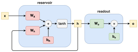
Figure 1.
Echo state network architecture.
An efficient and effective training function used to fit the readout is the ridge regression, a one-shot training function formalized in the following way:
where is the matrix of the output of the training set, is the matrix of the hidden states, is a vector of ones, and is the scalar Thikonov regularization hyperparameter ( represents the number of examples in the training set).
3.2. Long Short-Term Memory
LSTM [53] is often considered an advancement of RNNs [54]. While RNNs offered short-term memory capabilities, allowing the use of preceding information at a specific point in time for the ongoing task, LSTM takes this a step further. In contrast to RNNs, LSTM architecture introduces the concept of long-term memory, providing access to a comprehensive history of previous information rather than just a snapshot at a specific time. This extended memory capacity enhances the learning and decision-making capabilities of the neural network.
3.2.1. Long Short-Term Memory Model Efficiency
LSTMs overcome the limitations related to the short-term memory of RNNs by introducing the concept of long-term memory. To train LSTM models and recurrent models in general, the backpropagation through time (BPTT) algorithm is often used. This algorithm is known to be computationally expensive, as it involves backpropagation through the various time steps of the model, essentially treating the model as its “unrolled” version for each time step. This implies that the efficiency of BPTT directly depends on the number of time steps present in the time series being trained. However, it is important to note that training an LSTM model using BPTT may become impractical for IoT devices. These devices often have significant constraints in terms of memory and computing capacity. Deploying BPTT over long-term sequences can require computational and memory resources that exceed the capabilities of these devices, making it difficult or even impossible to implement such models on IoT platforms. Currently, computational problems are addressed using time-truncated backpropagation [55]. Despite its effectiveness in some contexts, BPTT is chosen due to its similarities with classical backpropagation [56]. This choice takes into account the computational constraints and resource limitations on IoT devices as well as the challenges associated with training over long time sequences.
3.2.2. LSTM Architecture
A typical LSTM model is illustrated in Figure 2. It comprises a cell, an input gate, an output gate, and a forget gate. Each of these components plays a crucial role in governing the flow of information within the network:
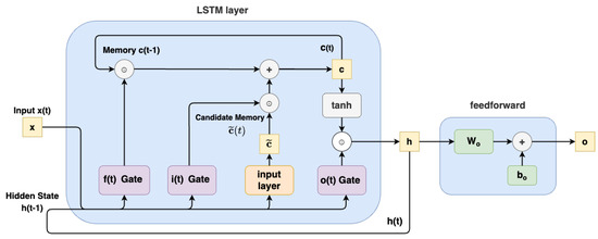
Figure 2.
Long short-term memory architecture.
- Cell State: This signifies the ongoing long-term memory of the network, retaining a list of past information.
- Previous Hidden State: This refers to the output from the preceding time point, akin to short-term memory.
- Input Data: This includes the input value of the current time step.
By incorporating these elements, the LSTM effectively manages both short-term and long-term memory, enabling more sophisticated learning and decision processes in neural networks (See Figure 2).
The recurrent part of LSTM is divided into three main gates (forget, input, and output), and each gate has the structure shown in Figure 3.
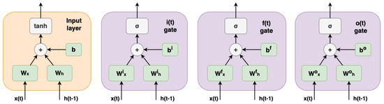
Figure 3.
Input layer and gates architecture.
A brief analysis of the different gates in the LSTM architecture is provided below. It is assumed that is the input of the system, and is the hidden state of the system.
3.2.3. Forget Gate
The forget gate plays a crucial role in determining the relevance of bits in the cell state. It evaluates both the previous hidden state and the new input data to generate a vector with elements in the interval [0,1] by means of a sigmoid activation function (). Trained to output values close to 0 for irrelevant components and close to 1 for relevant ones, the outputs of the forget gate are multiplied by the previous state of the cell. Mathematically, the results () of the forget gate are expressed as
where is the sigmoid activation function, is the input weights, is the recurrent weights, and is the bias of the forget gate.
3.2.4. Input Gate
The input gate has two purposes: First, it evaluates whether it is worth keeping the new information in the cell state, and second, it decides what new information to add. The gate involves two processes. The first process generates a new memory update vector by combining the previous hidden state and new input data using a tanh activation function. This vector determines how much each component of the cell state is updated. The process is expressed as
The second process identifies which components of the new input are worth remembering, given the context of the previous hidden state. Similar to the forget gate, the input gate outputs a vector of values in the interval [0,1] using the sigmoid activation function:
where is the sigmoid activation function, is the input weights, is the recurrent weights, and is the bias of the input gate. These processes are combined through point-wise multiplication (here, the ⊙ symbol), and the resulting vector is added to the cell state, updating the long-term memory:
3.2.5. Output Gate
After updating the long-term memory, the output gate determines the new hidden state. It uses the newly updated cell state, the previous hidden state, and the new input data. The output gate applies the previous hidden state and current input data through a sigmoid-activated network to obtain the filter vector . This vector is obtained as
where is the sigmoid activation function, is the input weights, is the recurrent weights, and is the bias of the output gate. The cell state undergoes a tanh activation function to create a squished cell state, which is then multiplied point wise (⊙ symbol) with the filter vector to create the new hidden state :
The new cell state becomes the previous cell state for the next LSTM unit, while the new hidden state becomes the previous hidden state for the subsequent LSTM unit. This process repeats until all time series sequences are processed by the LSTM cells.
3.2.6. Key Differences between LSTM and ESN
As mentioned above, LSTM networks are very powerful but computationally intensive models suitable for applications involving complex long-range dependencies, while ESNs offer a more computationally efficient alternative when speed and computational efficiency are paramount. Indeed, LSTMs require backpropagation through time (BPTT) to train both the recurrent and output layers, while the ESNs use a simpler training approach in which the recurrent part is not trained and only the output weights are adjusted in a one-shot learning function called ridge regression, avoiding the complexities of BPTT. The main advantages of using ESN are as follows:
- Fast training process
- Low computational cost
- Fairly simple implementation
- Suitable for real-time applications
4. Anomaly Detection Method Based on DeepESN
The proposed new AD methodology based on DeepESN is described in the following subsections.
4.1. Deep Echo State Network
A DeepESN model is shown in Figure 4. The DeepESN [57] is an echo state network model with more reservoir layers.
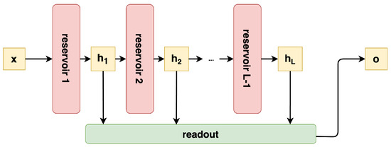
Figure 4.
Deep echo state network architecture.
Applying the deep learning paradigm [58] to the ESN model, it is possible to exploit multiple hidden states (one for each layer) related to different degrees of abstraction of the processed inputs. All of the reservoir layers are connected sequentially, meaning that the input of a deep reservoir layer is the hidden state of the previous one. All of the hidden states computed by all of the reservoirs are concatenated and passed to the readout for computing the prediction.
The DeepESN can be formalized by reusing the equations from Section 3.1.2, while the reservoir layers of the DeepESN can be formalized as follows:
where l is the number of layers, , and the hidden state of layer zero is the input time series. The readout maps the concatenation of the collection of all into the output prediction. It can be formalized as follows:
where , and the square parentheses represent the concatenation of the hidden state vectors in a unique vector with size . The ridge regression formula is the same as (3), where the only change is in terms of size, i.e., .
4.2. Anomaly Detector
The methodology introduced here aims to provide a way to detect anomalies in an unsupervised manner. The main architecture proposed is composed of two main parts: the deep learning model and the anomaly detector. The deep learning model is a RNN with a focus on comparing LSTM and ESN models and capable of performing a next-step prediction task taking as input and providing the prediction . The anomaly detector takes as input the prediction of the deep learning model , the related real input , and the standard deviation of errors of the training set and indicates class 0 for normal behavior or class 1 when it detects an anomaly. Going deeply into the anomaly detector (architecture shown in Figure 5), it performs the squared error between and and adds it to a queue of fixed size Q. To detect the anomaly, the standard deviation () of the queue Q is computed resulting in a vector of 1 and 0 according to the condition . A vector is provided for the detection of anomalies for each feature.
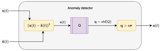
Figure 5.
Anomaly detector architecture.
4.3. DeepESN Anomaly Detection Architecture
The whole architecture proposed here is composed of the DeepESN model and the anomaly detector. The three phases that make up the global architecture are represented in Figure 6. To work in the inference phase, the anomaly detector requires and as hyperparameters. To compute them and determine the best hyperparameters for the construction of the DeepESN model, the model selection and the model assessment phase are performed. For both of them, three steps must be performed (see Figure 6), and these are called, respectively, model training, computation, and the evaluation phase. During model selection, the performances of different combinations of hyperparameters are registered together with a related metric result in order to determine the best hyperparameters for the DeepESN model and the best hyperparameter. In this phase, the training set is used to train the model and to compute , while the evaluation phase is run with the validation set. The true used in inference is computed in the model assessment phase. In the model assessment phase, after retraining the model, it is initialized using the best selected hyperparameters, and is computed on the training set. The final evaluation phase is performed on the test set to retrieve the final results of the method’s performance.
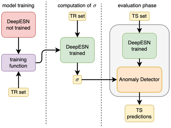
Figure 6.
The sub-phases in the global architecture of the proposed AD methodology.
The model training phase is described in Section 3 concerning preliminaries, while the computation of is conducted by taking the trained model and computing the prediction for each time series in the training set. Then, the predictions are compared with the true outputs to get the squared error. In the end, the standard deviation of all the squared errors, called , has been computed.
4.4. Key Benefits of the DeepESN Architecture
Compared with ESN, the DeepESN constrains the non-linear time series modeling capability of ESN by incorporating efficient deep learning functionality. The main advantages of using the DeepESN architecture are
- A deep layering of DeepESNs allows for the effective diversification of temporal representations in the layers of the hierarchy, amplifying the effects of the factors influencing the time scales and the richness of the dynamics, measured as the entropy of recurrent units’ activations [59].
- The short-term memory capacity of DeepESN is higher than that of ESN. The short-term memory capacity is used to determine how well the most recent data (input) can be remembered based on the current context [60]. The number of recurrent units is quite similar in both the DeepESN and ESN mechanisms. However, experiments have demonstrated that the DeepESN mechanism exhibits a higher short-term memory capacity than the basic ESN [61].
- The proposed DeepESN solution can be seen as a reduced form of the basic ESN model. Specifically, influences greater than one are eliminated from the initial layer to the reservoir, and connections between the higher layers and the lower states are removed, thereby ensuring fewer recurrent non-zero connections [62]. Furthermore, for both ESN and DeepESN (“layerization” of the ESN), the costs of updating each state are, respectively, and [63], where is the number of time steps, L the number of layers, and the size of the reservoir. Given that ESN is a “layerization” of DeepESN, its reservoir size is . DeepESN demonstrates significantly lower costs compared to the basic ESN system. In fact, DeepESN surpasses the basic ESN in both computational efficiency and accuracy.
Overall, the proposed DeepESN overcomes the standard ESN by increasing its computational efficiency, short-term memory capacity, and reservoir state richness. Accordingly, in this work it is proposed to use DeepESN to generate short-term predictions of electrical parameters. The general architecture of the proposed method, along with its associated input/output components, is depicted in Figure 7.
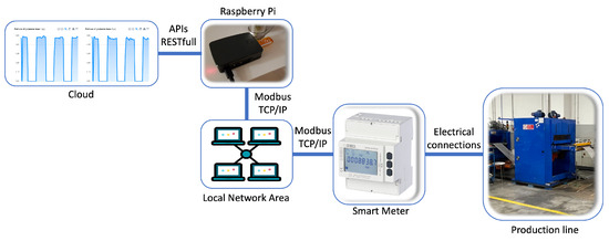
Figure 7.
System architecture.
4.5. Model Evaluation Metrics
The metrics proposed to quantify the obtained results can be divided into those that evaluate effectiveness and those that evaluate efficiency.
- Effectiveness metricsAll of the effectiveness metrics are executed on the test set. They are used to evaluate the entirety of the methodology performing a binary classification task. For this reason, we used the main metrics in binary classification scenarios, which are accuracy, precision, recall, and F1 score. The accuracy provides the percentage of correct predictions:where stands for true positive, for true negative, for false positive (1), and for false negative (0). The precision provides the percentage of true positives out of all positive predictions:The recall provides the percentage of true positives out of all positive real examples:The F1 score provides a balance between precision and recall:
- Efficiency metricsThe metrics used to evaluate the efficiency of the methodology include time-related measures and CO2 emissions. In terms of time, the seconds spent to train the model on the training set (training time) and those spent to predict all the results of the test set (inference time) have been measured. The time metric tells us how fast the model is during the training and inference phases. Additionally, the CO2 emissions are measured during the training phase and inference phase. This metric indicates the volume of carbon dioxide emissions (kgCO2) generated during the training and inference process. The CO2 emissions are computed starting from power resource consumption. Specifically, the emissions are measured using the codecarbon python library version 2.7.1, which allows for the registration of the kWh for the CPU and RAM of the device. kWh are converted into CO2 emissions by multiplying them by the carbon intensity of the current country in kg/kWh. The formula used is the following:and are monitored and measured during the run, while the country’s carbon intensity (cci) is a constant taken from the work in [64] where are the carbon intensity of each country is listed. In our case, the cci is 0.373 kg/kWh, which is the carbon intensity for Italy in the year 2022.
5. Experimental Setup
This section provides details of the experiment, including the real system hardware architecture, the devices involved in the proposed method, the environment setup, and the list of all energy variables acquired from the field. In detail, Section 5.1 describes the case study and the hardware on the edge, while in Section 5.1.1, the pilot case composed of a production line and the energy acquisition module is introduced. Subsequently, in Section 6, the data type and acquisition methods are highlighted.
5.1. Case Study
The proposed solution has been applied to a real test case composed of four actors that, when combined, allow for the creation of an infrastructure that can be replicated in many other industrial scenarios. The experimental setup consists of four actors. The first is the production line. It is the main system to be monitored in order to analyze the electrical parameters of the AD. The second actor is a smart meter module, which is directly connected both to the three-phase electrical connections of the industrial machine and to the third actor, the Raspberry Pi, using a Modbus TCP/IP protocol. The results of the AD are then sent to the fourth actor, the cloud, for further analysis and notification. In addition to this, to test and debug the proposed solution on the edge, the interconnection between the embedded device and the S604 module is not established directly but instead passes through the local area network (see Figure 7).
In the next paragraphs, the production line and the smart monitoring module are described.
5.1.1. Pilot Case
The proposed solution has been tested on a production line used for the production of metal filters by SIFIM Srl (Jesi, Ancona, Italy), an Italian company leader which specializes in the production of this type of component for the household appliances industry and community kitchen industry (restaurant, hotels, canteens, etc.). SIFIM’s production line can be divided into three functional blocks associated with the three production phases (See Figure 8):
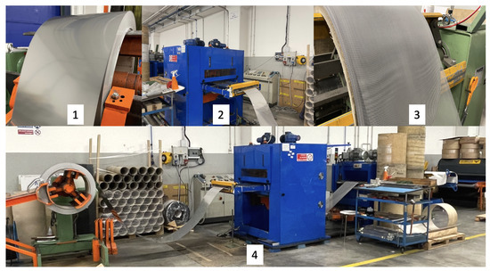
Figure 8.
Sifim’s production line. (1) Loading station. (2) Working area. (3) Unloading station. (4) Complete overview.
- Loading station: This is where the iron, steel, or aluminum sheet coil is loaded onto a decoiler.
- Work area: This is composed of a punching press that creates the weave of the metal mesh and a straightening area in which the mesh, passing through opposing rollers, is stretched and flattened.
- Unloading station: Here, a winding reel collects the coil of metal mesh produced.
The first and the third module are equipped with a 3 kw and kw three-phase asynchronous motor, respectively, while the second module uses four different types of motors: two three-phase asynchronous motors (one of kw for the main activity and the other of kw to manage the back-and-forth movement of the press in relation to the desired settings) and two brushless motors (2 kw and kw) used to control the oscillation and lateral displacement of the press head. The production line overall has an average consumption ranging from 5 to 8 amps depending on the type of material used to produce the filters and the production velocity (aluminum, stainless steel, etc.). In fact, even though the nominal power of the production line is over 25 kw, the actuators work only for a few milliseconds in a time range of one second.
5.1.2. Data Acquisition
The acquisition system has been chosen for the proposed approach based on the flexibility and manageability that an industrial monitoring system should have. Generally, a production line does not have a complete acquisition system containing all the information about the state of all variables involved in the process but instead exposes only a few details related to the production state, such as the production ID, the alarms, the on/off state, the number of items to be produced, etc. [65,66]. In addition to this, installing sensors on the production line can be expensive from an economic point of view and sometimes invasive in terms of wiring and CE certification. Based on these considerations, an energy IoT monitoring module, the S604 by Seneca [67], that includes a three-phase network analyzer, has been installed following the electrical connection guidelines as shown in Figure 9.
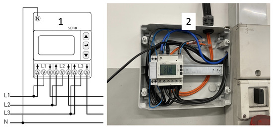
Figure 9.
Seneca S604’s IoT module. (1) Electric schema. (2) Installed module.
The module carries out one reading per second of over 250 different electrical parameters (current, voltage, power factor, displacement power factor, active energy, etc.) and performs calculations (every ten seconds) to define complex variables such as the minimum, maximum, or average value of another 150 variables. Furthermore, the harmonic calculation is performed every seven seconds. Due to the limited hardware resources, only 88 variables are acquired every second, as listed in Table 1.

Table 1.
List of acquired variables.
In the Figure 10, some values of the acquired variables during the operational tests are shown. Next, the data are saved in a csv file and organized by day in order prepare the dataset for feeding into the proposed model.
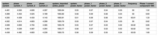
Figure 10.
Example of acquired data.
6. Materials and Methods
This section consists of a detailed explanation of the data and data preparation (Section 6.1), the hyperparameter settings (Section 6.2), and the model training and inference phase for the proposed solution (Section 6.3).
6.1. Data Preparation and Preprocessing
The raw data are represented by the matrix , where is the number of time steps during which each , where is the number of input features. The raw data come directly from the field, and in order to use them as an input for the model, it is important to prepare the data in a correct way. In fact, even though there are many available techniques for data scaling, choosing the best scaling method continues to be one of the most challenging problems because the performance of ML algorithms and the selection of standardization methods are interconnected [68,69,70]. For the proposed approach, based on the reduced computational resources available, six different types of data preparation are used:
- Data rectification:Generally, when the machine is not running, it is not turned off, and therefore, the data, such as voltage, frequency, etc., continue to have a non-zero value. Analyzing the data when the machine is not working, when the phase current is equal to zero, is useless for our purposes, so, in order to reduce the size of the time series, the data during the off period have been removed.
- Data cleaning:The whole dataset not only contains information about electrical parameters but also generic information such as serial numbers, IDs, and time information is not useful. This type of information does not support analysis of the anomaly estimation.
- Data operation:A type of data operation has been performed in order to adjust the values of the numerical columns of the dataset to a standard scale. Specifically, the data has been standardized to a probability distribution in which the mean is zero and the standard deviation is 1 according to Equation (17):where is the mean, and is the standard deviation of the time series.
- Dataset splitting:The dataset consisted of 269 time series () with 300 time steps () and 88 features (). The training set is about 60%, and the validation and test sets are about 20% and 20%, respectively.
- Data labeling:The validation and test sets present faults from halfway through the time series to the end. These anomalies are emulated by summing the noise with the original time series. The noise is generated from a normal distribution and is multiplied by 20% of the standard deviation of the dataset. Class 0 is used for no faults and Class 1 for the added faults.
6.2. Hyperparameter Settings
Based on the recommendations presented in [71,72], the hyperparameters for DeepESN and LSTM are obtained using the trial-and-error method. This method achieves satisfactory results by trying different hyperparameter combinations until the error is sufficiently reduced, which is effective and frequently used in hyperparameter setting [73,74]. This phase is called model selection, and the hyperparameter combinations are used to initialize and train new models on the training set and evaluate them on the validation set. In our case, being a binary classification method, instead of using an error minimization technique, we decided to leverage the accuracy metric in order to choose the best hyperparameter configuration that maximizes it (See Table 2).
Table 2.
Final best hyperparameter values.
6.3. Training Phase
In the initial training phase, several hyperparameters are explored for experimentation with the LSTM and DeepESN models. This in-depth analysis allows us to identify the optimal combination that leads to superior levels of accuracy. The optimal hyperparameters are identified through a targeted experimentation phase in order to maximize the performance of the LSTM and DeepESN models on the specific tasks to which they were applied. In the training phase, the model is adapted to predict the next step (next-step prediction). Training occurs using the training set, allowing the model to learn temporal relationships in the input data. In particular, for LSTM, the mean squared error (MSE) is used as the loss function, and Adam is used as the optimizer, while for DeepESN, the learning function is the one-shot ridge regression learning rule. After training, the next step is the calculation of errors in the training set, measuring the discrepancy between the model predictions and the respective time steps of the training set. These errors are recorded in a buffer, and the standard deviation is generated. This step is crucial for the dynamic calculation of the sigma value, which will subsequently be used to verify anomalies. The standard deviation of the errors of the time steps of the training set () and of the queue (queue, ) is not a single value but a vector of standard deviations, each associated with a specific feature (in our case, a composite vector from the 88 features of the time series). This approach allows for more accurate anomaly detection, since the detection process is performed separately for each feature in the time series. A visual representation of vectors is shown in Figure 11.
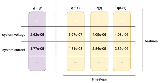
Figure 11.
Example of and vectors.
Inference Phase
During this phase, the trained model is combined with the anomaly detector to work in a real case. This phase is described by Algorithm 1.
In this scenario, each time a new time step arrives in the stream, it is processed by the deep learning model, which provides the prediction of the next step. The result is passed to the anomaly detector with the real value of the next step, which arrives in the following moment. The anomaly detector generates , the vector that contains the predictions of anomalies for each feature at time step t. Fixing a certain threshold , a general anomaly can be identified when more features than the threshold are detected as failures.
| Algorithm 1 Inference phase pseudocode | |
| standard deviation of errors in the training set | |
| hyperparameter related to the threshold of standard deviation error | |
| Q queue of last errors | |
| M trained model (DeepESN or LSTM) | |
| threshold of feature detected to send a notification of the anomaly | |
| for new input do | |
| next step prediction | |
| computation of current error | |
| addition of error in the queue Q | |
| computation of standard deviation of Q | |
| anomaly detection for each feature | |
| if then | |
| send_notification() | |
| end if | |
| end for | |
7. Results and Discussion
Experimental results are discussed in this section as well as comparative analysis among low-level and high-level models. In Table 3, the results of each metric described in Section 4.5 for the use of the DeepESN (our proposal) and LSTM (state-of-the-art) models in combination with the anomaly detector are described.
Table 3.
Results for individual metrics with the use of DeepESN and LSTM deep-learning models.
The first results are related to effectiveness, while the latter results are related to efficiency. Regarding effectiveness metrics, our proposal is better than the state-of-the-art in terms of accuracy, recall, and F1 score, respectively, by around 2%, 9%, and 4%, while is worse in terms of precision by around 5%. In general, from the point of view of effectiveness, the use of DeepESN brings about better results than LSTM, except in terms of precision. In terms of efficiency, the use of DeepESN is better than the LSTM model. The time measured in training is improved by three orders of magnitude, while the time spent in inference is less than one-third of the state-of-the-art. Regarding CO2 emissions, our proposal outperforms the state-of-the-art by two orders of magnitude in the training phase and one order of magnitude in the inference phase. Efficiency results prove that our proposal is highly efficient with respect to the state-of-the-art. This consideration promotes the usage of our proposal directly in on-the-edge devices instead of exploiting a remote server both for training and inference. The LSTM model is trained using the backpropagation through time (BPTT) algorithm, while the DeepESN model uses the ridge regression algorithm. BPTT is iterative (the iterations of the algorithm are called epochs), while ridge regression is one-shot. In the following analysis, the performance of the LSTM model combined with the anomaly detector during the iterations of training is compared with the one-shot-trained DeepESN.
Figure 12 shows the evolution of accuracy and F1 score for the effectiveness metrics and time and CO2 emissions for the efficiency metrics. In all the plots, the x-axis is related to the epochs of the BPTT training algorithm, while the y-axis is related to the analyzed metric. The accuracy and F1 score metrics are computed on the test set, and they show that DeepESN outperforms LSTM at each epoch of training. In terms of efficiency, a low result is desired for both time and CO2 emissions. Both in terms of time and CO2 emissions, the LSTM is inefficient at the first epoch. Over the course of subsequent epochs, which bring with them an improvement in effectiveness, the methodology becomes more and more expensive, with a linear increase. The inefficiency of the BPTT algorithm promotes its usage inside of a server, while our proposal can be implemented directly inside of on-the-edge devices due to its good efficiency. In order to emphasize the results obtained, a graphic visualization has been chosen. In the representation, the left side of the graph offers a comparison between the two models, DeepESN and LSTM, regarding standard deviation.
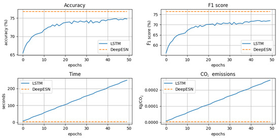
Figure 12.
Development of the accuracy, F1 score, time, and CO2 emissions metrics for each epoch of LSTM model training compared with the one-shot DeepESN results.
In the legend, the standard deviation values are indicated as follows:
- q: Standard deviation of the error.
- Anomaly threshold: This represents the average of the values used to calculate the upper (+). This dashed green band indicates the range in which the standard deviation of the error must remain in order to prevent a failure from occurring.
- Actual anomaly: This indicates the start of the actual anomaly.
- Predicted anomaly: This indicates the start of the predicted anomaly.
On the right-hand side of the graph, the time series values are presented, with the following legend:
- Effective time series: This represents the actual trend of the time series.
- Predicted time series: This shows the predicted trend of the time series.
- Actual anomaly: This indicates the start of the actual anomaly.
- Predicted anomaly: This signals the start of the predicted anomaly.
This visual representation provides a clear comparison between the two models in terms of standard deviation and offers a detailed overview of the temporal trend of the time series, highlighting both actual and predicted anomalies. The analysis begins by focusing on the system current as the first feature. As highlighted in Figure 13, although both models show a similar trend in the time series, the DeepESN presents timelier error detection. The prediction of the time series by DeepESN has a slightly more indented behavior than the LSTM model. DeepESN allows us to find the fault before LSTM because after the effective fault, the prediction starts to look very different from the effective time series.
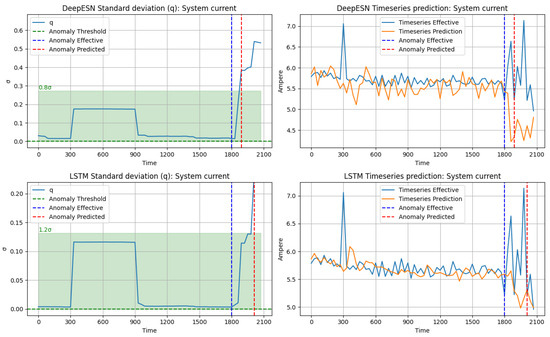
Figure 13.
Current system anomaly detection.
A further indicator used to evaluate the performance of the proposed model is the confusion matrix (CM), which allows for the calculation of metrics such as precision, recall, and accuracy, providing a detailed view of the classification errors. As shown in Table 4, the percentage of is higher than , confirming the lower value of recall with respect to precision.
Table 4.
DeepESN confusion matrix.
Another useful indicator is the receiver operating characteristic (ROC) curve shown in Figure 14. It shows that the model is effective in distinguishing between positive and negative instances.
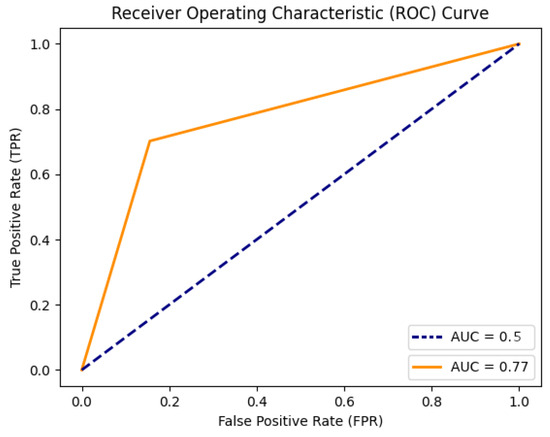
Figure 14.
DeepESN receiver operating characteristic (ROC) curve.
Indeed, the area under the curve (AUC) score, equal to , further quantifies its performance, showing that the proposed model correctly ranks a randomly chosen positive instance higher than a negative instance of the time.
8. Conclusions
This work presented a novel methodology for anomaly detection, leveraging the combination of a deep learning model and an anomaly detector. The deep learning model, implemented as a RNN, was compared with both LSTM and DeepESN architectures, with our findings demonstrating the superiority of the proposed DeepESN approach. This architecture proved to be not only efficient but also faster and lightweight, making it well-suited for deployment on resource-constrained embedded devices at the edge. The anomaly detector, a critical component of our framework, exhibited its effectiveness in distinguishing normal behavior from anomalies based on the comparison of predicted and real inputs, further augmented by the standard deviation of errors. The three-phase model selection and model assessment approach facilitated the identification of optimal hyperparameters, ensuring the robustness and adaptability of the deep learning model. The introduction of DeepESN, a hybrid model combining efficient deep learning functionality with the strengths of ESN, proved advantageous. DeepESN exhibited enhanced temporal representation diversification, powerful short-term memory capacity, and amplified computing efficiency compared to the baseline ESN mechanism. These advantages position DeepESN as a formidable choice for the short-term forecasting of electrical parameters within our proposed methodology. Experimental results showcased the effectiveness and efficiency of our proposal, particularly when compared to the state-of-the-art LSTM model. Despite the slight superiority of LSTM in the mean squared error metric, our approach demonstrated comparable effectiveness metrics, with notable improvements in efficiency. The significant reduction in training time and CO2 emissions highlights the potential environmental and cost benefits of our proposed methodology. In summary, our comprehensive evaluation demonstrates the feasibility and advantages of our proposed approach, making it a compelling solution for on-the-edge deployment, directly addressing the limitations of traditional server-based implementations. The proposed methodology, grounded in the robustness of DeepESN and the efficiency of the anomaly detector, sets the stage for advancements in real-time anomaly detection on resource-constrained devices at the edge of the network. However, although the initial findings are promising, there is still a need for further exploration with objectives such as:
- Monitoring the production line as different types of items are manufactured, linking time-series data to the specific products being produced;
- Labeling all types of faults and malfunctions to continuously improve the performance of the AD model;
- Implementing a continuous learning technique to enable the model to update itself and adapt to temporal changes in the degradation of the production line.
Author Contributions
Methodology, A.B., M.P. and S.L.; validation, A.B., M.P., G.P. and L.L.; formal analysis, A.B. and M.P.; investigation, M.P., L.F., R.K., G.P. and L.L.; resources, M.P., G.P., L.F., R.K., L.L., A.B. and C.V.; data curation, G.P., L.L. and C.V.; writing—original draft preparation, M.P., G.P. and L.L.; writing—review and editing, A.B. and M.P.; visualization, A.B. and M.P.; supervision, M.P., A.B. and S.L.; project administration, A.B. and M.P. All authors have read and agreed to the published version of the manuscript.
Funding
This research has been supported by Italian PON “RICERCA E INNOVAZIONE” 2014-2020-AZIONE IV.6 “CONTRATTI DI RICERCA SU TEMATICHE GREEN”, and it was partially funded by the European project Horizon Europe “EDIH4Marche” (European Digital Innovation Hub for Marche), Call DIGITAL-2021-EDIH-01, Grant Agreement no. 101084027 on topic DIGITAL-2021-EDIH-INITIAL-01 (DIGITAL Simple Grants Acton).
Data Availability Statement
The original contributions presented in the study are included in the article, further inquiries can be directed to the corresponding author.
Acknowledgments
A special acknowledgment is given to Sifim Srl for their willingness to install a smart meter sensor on their production line, and sincere thanks is offered to Syncode Scarl for their crucial support in a significant research project, providing both the essential hardware devices and software infrastructure.
Conflicts of Interest
Author Carlo Verdini was employed by the company Syncode Scarl. The remaining authors declare that the research was conducted in the absence of any commercial or financial relationships that could be construed as a potential conflict of interest.
Abbreviations
The following abbreviations are used in this manuscript:
| AD | Anomaly Detection |
| AE | Autoencoder Neural Networks |
| BiGAN | Bidirectional GAN |
| BPTT | Backpropagation Through Time |
| CNN | Convolutional Neural Network |
| DeepESN | Deep Echo State Network |
| ESN | Echo State Network |
| ESP | Echo State Property |
| GAN | Generative Adversarial Network |
| GHG | Greenhouse Gas |
| IIoT | Industrial Internet of Things |
| IoT | Internet of Things |
| LSTM | Long Short-Term Memory |
| ML | Machine Learning |
| MLP | Multilayer Perceptron |
| PdM | Predictive Maintenance |
| OEEE | Overall Environmental Equipment Effectiveness |
| RNN | Recurrent Neural Network |
| RUL | Remaining Useful Life |
| SWCVAE | Sliding-Window Convolutional Variational Autoencoder |
References
- Domingo, R.; Marin, R.R.; Claver, J.; Calvo, C. Climate change and COP26: Are digital technologies and information management part of the problem or the solution? An editorial reflection and call to action. Int. J. Inf. Manag. 2022, 63, 0268–4012. [Google Scholar]
- Zou, J.; Chang, Q.; Ou, X.; Arinez, J.; Xiao, G. Resilient adaptive control based on renewal particle swarm optimization to improve production system energy efficiency. Int. J. Manuf. Syst. 2019, 50, 135–145. [Google Scholar] [CrossRef]
- Chang, Q.; Xiao, G.; Biller, S.; Li, L. Energy saving opportunity analysis of automotive serial production systems. IEEE Trans. Autom. Sci. Eng. 2012, 63, 334–342. [Google Scholar]
- Henao, H.; Capolino, G.-A.; Fernandez-Cabanas, M.; Filippetti, F.; Bruzzese, C.; Strangas, E.; Pusca, R.; Estima, J.; Riera-Guasp, M.; Hedayati-Kia, S. Trends in fault diagnosis for electrical machines: A review of diagnostic techniques. IEEE Ind. Electron. Mag. 2014, 8, 31–42. [Google Scholar] [CrossRef]
- Bonci, A.; Longhi, S.; Nabissi, G. Fault Diagnosis in a belt-drive system under non-stationary conditions. An industrial case study. In Proceedings of the 2021 IEEE Workshop on Electrical Machines Design, Control and Diagnosis (WEMDCD), Modena, Italy, 8–9 April 2021; pp. 260–265. [Google Scholar]
- Nandi, S.; Toliyat, H.A.; Li, X. Condition monitoring and fault diagnosis of electrical motors—A review. IEEE Trans. Energy Convers. 2005, 20, 719–729. [Google Scholar] [CrossRef]
- Gordic, D.; Babic, M.; Jovicic, N.; Sustersic, V.; Koncalovic, D.; Jelic, D. Development of an energy management system—Case study of a Serbian car manufacturer. J. Energy Convers. Manag. 2010, 50, 2783–2790. [Google Scholar] [CrossRef]
- Zhang, Q.; Li, Y.; Xu, J.; Jia, G. Carbon element flow analysis and CO2 emission reduction in iron and steel works. J. Clean. Prod. 2018, 20, 709–723. [Google Scholar] [CrossRef]
- Domingo, R.; Marin, M.M.; Claver, J.; Calvo, R. Selection of cutting inserts in dry machining for reducing energy consumption and CO2 emissions. J. Energies 2015, 11, 13081–13095. [Google Scholar] [CrossRef]
- Bonci, A.; Di Biase, A.; Dragoni, A.F.; Longhi, S.; Sernani, P.; Zega, A. Machine learning for monitoring and predictive maintenance of cutting tool wear for clean-cut machining machines. In Proceedings of the IEEE 27th International Conference on Emerging Technologies and Factory Automation (ETFA), Stuttgart, Germany, 6–9 September 2022; pp. 1–8. [Google Scholar]
- Rajemi, M.F.; Mativenga, P.T.; Aramcharoen, A. Sustainable machining: Selection of optimum turning conditions based on minimum energy considerations. J. Clean. Prod. 2010, 18, 1059–1065. [Google Scholar] [CrossRef]
- Campatelli, G.; Lorenzini, L.; Scippa, A. Optimization of process parameters using a response surface method for minimizing power consumption in the milling of carbon steel. J. Clean. Prod. 2014, 66, 309–316. [Google Scholar] [CrossRef]
- Abdelaziz, E.A.; Saidur, R.; Mekhilef, S. A review on energy saving strategies in industrial sector. J. Renew. Sustain. Energy Rev. 2011, 15, 150–168. [Google Scholar] [CrossRef]
- Cercós, M.P.; Calvo, L.M.; Domingo, R. An exploratory study on the relationship of Overall Equipment Effectiveness (OEE) variables and CO2 emissions. J. Procedia Manuf. 2019, 41, 224–232. [Google Scholar] [CrossRef]
- Bonci, A.; Stadnicka, D.; Longhi, S. The Overall Labour Effectiveness to Improve Competitiveness and Productivity in Human-Centered Manufacturing. In Proceedings of the International Scientific-Technical Conference Manufacturing, Poznan, Poland, 16–19 May 2022; pp. 144–155. [Google Scholar]
- Susto, G.A.; Beghi, A.; De Luca, C. A Predictive Maintenance System for Epitaxy Processes Based on Filtering and Prediction Techniques. IEEE Trans. Semicond. Manuf. 2012, 25, 638–649. [Google Scholar] [CrossRef]
- Liao, R.; He, Y.; Feng, T.; Yang, X.; Dai, W.; Zhang, W. Mission reliability-driven risk-based predictive maintenance approach of multistate manufacturing system. J. Reliab. Eng. Syst. Saf. 2023, 236, 109273. [Google Scholar] [CrossRef]
- Ariyo, A.A.; Adewumi, A.O.; Ayo, C.K. Stock Price Prediction Using the ARIMA Model. In Proceedings of the 16th International Conference on Computer Modelling and Simulation, Cambridge, UK, 26–28 March 2014; pp. 106–112. [Google Scholar]
- Anderson, M.L.; Chen, Z.-Q.; Kavvas, M.L.; Feldman, A. Coupling HEC-HMS with Atmospheric Models for Prediction of Watershed Runoff. J. Hydrol. Eng. 2002, 7, 312–318. [Google Scholar] [CrossRef]
- Alharbi, F.R.; Csala, D. A Seasonal Autoregressive Integrated Moving Average with Exogenous Factors (SARIMAX) Forecasting Model-Based Time Series Approach. Inventions 2022, 7, 94. [Google Scholar] [CrossRef]
- Susto, G.A.; Beghi, A.; De Luca, C. Prognostic modelling options for remaining useful life estimation by industry. J. Mech. Syst. Signal Process. 2011, 25, 1803–1836. [Google Scholar]
- Prytz, R.; Nowaczyk, S.; Rögnvaldsson, T.; Byttner, S. Predicting the need for vehicle compressor repairs using maintenance records and logged vehicle data. J. Eng. Appl. Artif. Intell. 2015, 41, 139–150. [Google Scholar] [CrossRef]
- Zenisek, J.; Holzinger, F.; Affenzeller, M. Machine learning based concept drift detection for predictive maintenance. J. Comput. Ind. Eng. 2019, 137, 106031. [Google Scholar] [CrossRef]
- Haibin, C.; Tan, P.N.; Potter, C.; Klooster, S. Detection and characterization of anomalies in multivariate time series. In Proceedings of the 2009 SIAM International Conference on Data Mining, Sparks, Nevada, 30 April–2 May 2009; pp. 413–424. [Google Scholar]
- Seyr, H.; Muskulus, M.; Klooster, S. Use of Markov Decision Processes in the Evaluation of Corrective Maintenance Scheduling Policies for Offshore Wind Farms. J. Energies 2019, 12, 2993. [Google Scholar] [CrossRef]
- Erguido, A.; Marquez, A.C.; Castellano, E.; Fernandez, J.F.G. A dynamic opportunistic maintenance model to maximize energy-based availability while reducing the life cycle cost of wind farms. J. Energies 2017, 114, 843–856. [Google Scholar] [CrossRef]
- Hajej, Z.; Nidhal, R.; Anis, C.; Bouzoubaa, M. An optimal integrated production and maintenance strategy for a multi-wind turbines system. Int. J. Prod. Res. 2020, 58, 6417–6440. [Google Scholar] [CrossRef]
- Pradhan, P.; Kishore, S.; Defourny, B. Optimal Predictive Maintenance Policy for an Ocean Wave Farm. IEEE Trans. Sustain. Energy 2019, 10, 1993–2004. [Google Scholar] [CrossRef]
- Xia, T.B.; Xi, L.F.; Du, S.C.; Xiao, L.; Pan, E.S. Energy-Oriented Maintenance Decision-Making for Sustainable Manufacturing Based on Energy Saving Window. J. Manuf. Sci. Eng.-Trans. ASME 2018, 140, 051001. [Google Scholar] [CrossRef]
- Dong, Y.; Japkowicz, N. Threaded ensembles of autoencoders for stream learning. J. Comput. Intell. 2017, 34, 261–281. [Google Scholar] [CrossRef]
- Yu, K.; Shi, W.; Santoro, N. Designing a Streaming Algorithm for Outlier Detection in Data Mining—An Incremental Approach. J. Sensors 2020, 20, 1261. [Google Scholar] [CrossRef]
- Song, L.; Liang, H.; Zheng, T. Real-Time Anomaly Detection Method for Space Imager Streaming Data Based on HTM Algorithm. In Proceedings of the 2019 IEEE 19th International Symposium on High Assurance Systems Engineering (HASE), Hangzhou, China, 3–5 January 2019; Volume 20, pp. 33–38. [Google Scholar]
- Moghaddass, R.; Sheng, S. An anomaly detection framework for dynamic systems using a Bayesian hierarchical framework. J. Appl. Energy 2019, 240, 561–582. [Google Scholar] [CrossRef]
- Kroll, B.; Schaffranek, D.; Schriegel, S.; Niggemann, O. System modeling based on machine learning for anomaly detection and predictive maintenance in industrial plants. In Proceedings of the 2014 IEEE Emerging Technology and Factory Automation (ETFA), Barcelona, Spain, 16–19 September 2014; pp. 1–7. [Google Scholar]
- Bonci, A.; De Amicis, R.; Longhi, S.; Lorenzoni, E.; Scala, G.A. Motorcycle’s lateral stability issues: Comparison of methods for dynamic modelling of roll angle. In Proceedings of the 2016 20th International Conference on System Theory, Control and Computing (ICSTCC), Sinaia, Romania, 13–15 October 2016; pp. 607–612. [Google Scholar]
- Bonci, A.; Longhi, S.; Scala, G.A. Towards an All-Wheel Drive Motorcycle: Dynamic Modeling and Simulation. IEEE Access 2020, 8, 112867–112882. [Google Scholar] [CrossRef]
- Kermenov, R.; Nabissi, G.; Longhi, S.; Bonci, A. Anomaly Detection and Concept Drift Adaptation for Dynamic Systems: A General Method with Practical Implementation Using an Industrial Collaborative Robot. Sensors 2023, 23, 3260. [Google Scholar] [CrossRef]
- Patti, G.; Alderisi, G.; Bello, L.L. SchedWiFi: An Innovative Approach to support Scheduled Traffic in Ad-hoc Industrial IEEE 802.11 networks. In Proceedings of the 2015 IEEE 20th Conference on Emerging Technologies and Factory Automation (ETFA), Luxembourg, 8–11 September 2015. [Google Scholar]
- Bonci, A.; Longhi, S.; Nabissi, G.; Scala, G.A. Execution Time of Optimal Controls in Hard Real Time, a Minimal Execution Time Solution for Nonlinear SDRE. IEEE Access 2020, 8, 158008–158025. [Google Scholar] [CrossRef]
- Manaswi, N.K.; John, S. Deep Learning with Applications Using Python; Apress: Berkeley, CA, USA, 2018. [Google Scholar]
- Wang, Z.; Chen, Z.; Ni, J.; Liu, H.; Chen, H.; Tang, J. Multi-scale one-class recurrent neural networks for discrete event sequence anomaly detection. In Proceedings of the 27th ACM SIGKDD International Conference on Knowledge Discovery and Data Mining, Virtual Event, 14–18 August 2021; pp. 3726–3734. [Google Scholar]
- Kingmaand, D.P.; Welling, M. Auto-encoding variational Bayes. arXiv 2014, arXiv:1312.6114. [Google Scholar]
- Chen, T.; Liu, X.; Xia, B.; Wang, W.; Lai, Y. Unsupervised anomaly detection of industrial robots using sliding-window convolutional variational autoencoder. IEEE Access 2020, 8, 47072–47081. [Google Scholar] [CrossRef]
- Chakraborty, D.; Narayanan, V.; Ghosh, A. Integration of deep feature extraction and ensemble learning for outlier detection. Pattern Recognit. 2019, 89, 161–171. [Google Scholar] [CrossRef]
- Goodfellow, I.J.; Pouget-Abadie, J.; Mirza, M.; Xu, B.; Warde-Farley, D.; Ozair, S.; Courville, A.; Bengio, Y. Generative adversarial networks. Adv. Neural Inf. Process. Syst. 2014, 27. [Google Scholar] [CrossRef]
- Akcay, S.; Atapour-Abarghouei, A.; Breckon, T.P. Ganomaly: Semisupervised anomaly detection via adversarial training. In Proceedings of the Asian Conference on Computer Vision, Perth, Australia, 2–6 December 2018; pp. 622–637. [Google Scholar]
- Zenati, H.; Foo, C.S.; Lecouat, B.; Manek, G.; Chandrasekhar, V.R. Efficient ganbased anomaly detection. arXiv 2018, arXiv:1802.06222. [Google Scholar]
- Donahue, J.; Krähenbühl, P.; Darrell, T. Adversarial feature learning. arXiv 2016, arXiv:1605.09782. [Google Scholar]
- Jaeger, H.; Haas, H. Harnessing Nonlinearity: Predicting Chaotic Systems and Saving Energy in Wireless Communication. J. Sci. 2004, 304, 78–80. [Google Scholar] [CrossRef]
- Schmidt, R.M. Recurrent Neural Networks (RNNs): A gentle Introduction and Overview. arXiv 2019, arXiv:1912.05911. [Google Scholar]
- Verstraeten, D.; Schrauwen, B.U.; D’Haene, M.; Stroobandt, D. An experimental unification of reservoir computing methods. J. Neural Netw. 2007, 20, 391–403. [Google Scholar] [CrossRef]
- Werbos, P.J. Backpropagation through time: What it does and how to do it. Proc. IEEE 1990, 78, 1550–1560. [Google Scholar] [CrossRef]
- Yu, Y.; Si, X.; Hu, C.; Zhang, J. A Review of Recurrent Neural Networks: LSTM Cells and Network Architectures. Neural Comput. 2019, 31, 1235–1270. [Google Scholar] [CrossRef]
- Sherstinsky, A. Fundamentals of Recurrent Neural Network (RNN) and Long Short-Term Memory (LSTM) network. Phys. Nonlinear Phenom. 2020, 404, 132306. [Google Scholar] [CrossRef]
- Williams, R.J.; Peng, J. An efficient gradient-based algorithm for on-line training of recurrent network trajectories. Neural Comput. 1990, 2, 490–501. [Google Scholar] [CrossRef]
- Hecht-Nielsen, R. Theory of the Backpropagation Neural Network; Academic Press: Cambridge, MA, USA, 1992. [Google Scholar]
- Gallicchio, C.; Micheli, A. Deep Echo State Network (DeepESN): A Brief Survey. arXiv 2017, arXiv:1712.04323. [Google Scholar]
- Schmidhuber, J. Deep learning in neural networks: An overview. J. Neural Netw. 2015, 61, 85–117. [Google Scholar] [CrossRef]
- Gallicchio, C.; Micheli, A.; Pedrelli, L. Deep reservoir computing: A critical experimental analysis. J. Neurocomput. 2017, 268, 88–99. [Google Scholar] [CrossRef]
- Jaeger, H. Short Term Memory in Echo State Networks; GMD Forschungszentrum Informationstechnik: Sankt Augustin, Germany, 2001. [Google Scholar]
- Jaeger, H.; Lukoševičius, M.; Popovici, D.; Siewert, U. Optimization and applications of echo state networks with leaky-integrator neurons. J. Neural Netw.-Sci. 2007, 20, 335–352. [Google Scholar] [CrossRef]
- Gallicchio, C.; Micheli, A. Echo state property of deep reservoir computing networks. J. Cogn. Comput. 2017, 9, 337–350. [Google Scholar] [CrossRef]
- Gallicchio, C.; Micheli, A. Why Layering in Recurrent Neural Networks? A DeepESN Survey. In Proceedings of the International Joint Conference on Neural Networks (IJCNN), Rio de Janeiro, Brazil, 8–13 July 2018; pp. 1–8. [Google Scholar]
- Ritchie, H.; Rosado, P.; Roser, M. Energy. 2023. Available online: https://ourworldindata.org/ (accessed on 16 September 2024).
- Prist, M.; Longhi, S.; Monteriù, A.; Giuggioloni, F.; Freddi, A. An integrated simulation environment for Wireless Sensor Networks. In Proceedings of the IEEE 16th International Symposium on a World of Wireless, Mobile and Multimedia Networks (WoWMoM), Boston, MA, USA, 14–17 June 2015; Volume 4, pp. 1–5. [Google Scholar]
- Grisostomi, M.; Ciabattoni, L.; Prist, M.; Ippoliti, G.; Longhi, S. Application of a wireless sensor networks and Web2Py architecture for factory line production monitoring. In Proceedings of the IEEE 11th International Multi-Conference on Systems, Signals & Devices (SSD14), Castelldefels-Barcelona, Spain, 11–14 February 2014; pp. 1–6. [Google Scholar]
- Seneca S604 Smart Meter Portal. Available online: https://www.seneca.it/media/4166/power_1912eng_r1.pdf (accessed on 4 December 2023).
- Ambarwari, A.; Adrian, Q.J.; Herdiyeni, Y. Analysis of the Effect of Data Scaling on the Performance of the Machine Learning Algorithm for Plant Identification. J. RESTI (Rekayasa Sist. Dan Teknol. Inf.) 2020, 4, 117–122. [Google Scholar] [CrossRef]
- Shahriyari, L. Effect of normalization methods on the performance of supervised learning algorithms applied to HTSeq-FPKM-UQ data sets: 7SK RNA expression as a predictor of survival in patients with colon adenocarcinoma. J. Briefings Bioinform. 2019, 20, 985–994. [Google Scholar] [CrossRef]
- Ahsan, M.M.; Mahmud, M.A.P.; Saha, P.K.; Gupta, K.D.; Siddique, Z. Effect of Data Scaling Methods on Machine Learning Algorithms and Model Performance. J. Technol. 2021, 9, 52. [Google Scholar] [CrossRef]
- Valencia, C.H.; Vellasco, M.M.B.R.; Figueiredo, K. Echo State Networks: Novel reservoir selection and hyperparameter optimization model for time series forecasting. J. Neurocomput. 2023, 545, 126–137. [Google Scholar] [CrossRef]
- Li, W.; Ng, W.; Wang, T.; Pelillo, M.; Kwong, S. HELP: An LSTM-based approach to hyperparameter exploration in neural network learning. J. Neurocomput. 2021, 442, 161–172. [Google Scholar] [CrossRef]
- Xu, M.; Meng, Q.; Huang, Z. Global convergence of the trial-and-error method for the traffic-restraint congestion-pricing scheme with day-to-day flow dynamics. J. Transp. Res. Part Emerg. Technol. 2016, 69, 276–290. [Google Scholar] [CrossRef]
- Ivanyos, G.; Kulkarni, R.; Qiao, Y.; Santha, M.; Sundaram, A. On the complexity of trial and error for constraint satisfaction problems. J. Comput. Syst. Sci. 2018, 92, 48–64. [Google Scholar] [CrossRef]
Disclaimer/Publisher’s Note: The statements, opinions and data contained in all publications are solely those of the individual author(s) and contributor(s) and not of MDPI and/or the editor(s). MDPI and/or the editor(s) disclaim responsibility for any injury to people or property resulting from any ideas, methods, instructions or products referred to in the content. |
© 2024 by the authors. Licensee MDPI, Basel, Switzerland. This article is an open access article distributed under the terms and conditions of the Creative Commons Attribution (CC BY) license (https://creativecommons.org/licenses/by/4.0/).