Abstract
At present, data-driven fault diagnosis has made significant achievements. However, in actual industrial environments, labeled fault data are difficult to obtain, making the industrial application of intelligent fault diagnosis models very challenging. This limitation even prevents intelligent fault diagnosis algorithms from being applicable in real-world industrial settings. In light of this, this paper proposes a Collaborative Domain Adversarial Network (CDAN) method for the fault diagnosis of rolling bearings using unlabeled data. First, two types of feature extractors are employed to extract features from both the source and target domain samples, reducing signal redundancy and avoiding the loss of critical signal features. Second, the multi-kernel clustering algorithm is used to compute the differences in input feature values, create pseudo-labels for the target domain samples, and update the CDAN network parameters through backpropagation, enabling the network to extract domain-invariant features. Finally, to ensure that unlabeled target domain data can participate in network training, a pseudo-label strategy using the maximum probability label as the true label is employed, addressing the issue of unlabeled target domain data not being trainable and enhancing the model’s ability to acquire reliable diagnostic knowledge. This paper validates the CDAN using two publicly available datasets, CWRU and PU. Compared with four other advanced methods, the CDAN method improved the average recognition accuracy by 7.85% and 5.22%, respectively. This indirectly proves the effectiveness and superiority of the CDAN in identifying unlabeled bearing faults.
1. Introduction
Bearings are a critical support component in mechanical transmission systems, and their fault diagnosis is key to ensuring the safe operation of equipment and avoiding economic losses. Numerous intelligent fault diagnosis methods have emerged in the research of bearing fault diagnosis [1,2]. In the early stages of intelligent fault diagnosis for bearings, scholars proposed diagnostic methods based on shallow machine learning, including extreme learning machines, support vector machines, and Bayesian methods [3,4]. In recent years, the accuracy of traditional unsupervised learning methods such as clustering, feature statistics, and random forests in identifying mechanical faults has been significantly lower than that of supervised learning neural networks in fault diagnosis [5,6,7], attracting widespread attention from both industry and academia. Particularly, deep learning, as a representative data-driven method, has been successfully applied to the field of mechanical equipment fault diagnosis. However, supervised deep learning methods have certain limitations, such as the need for sufficient and complete labeled fault samples and the requirement that the distribution of fault sample features used for training is consistent with the distribution of real fault sample features [8,9]. In actual industrial production, due to the variable operating states of equipment such as load, speed, and torque, as well as the impact of mechanical wear and external noise variations, the original vibration signals exhibit different feature distributions. Moreover, most of the collected data are unlabeled, and obtaining a complete labeled fault dataset is very difficult and requires significant human and material resources [10].
Many scholars have conducted extensive research in solving the problem of unlabeled equipment fault diagnosis [11,12,13]. The domain adversarial adaptive method is a transfer learning approach that has made significant contributions to solving the problem of fault recognition with few training samples and missing labels [14]. Jiao et al. [15] proposed an adversarial adaptive network with periodic feature alignment to facilitate transferable feature learning. Additionally, numerous researchers have integrated both approaches to enhance diagnostic performance [16,17]. Ganin et al. [18] proposed transfer learning by adding domain discriminators on the basis of Adversarial Generative Networks (GANs). For various types of transfer tasks, the transfer learning can be divided into subdomain transfer learning [19], closed domain transfer learning [20], multi-source domain transfer learning, etc. Xu et al. [21] proposed an unsupervised transfer learning model for multi-source domains by transferring multiple sets of source domain data to the target domain. In order to solve the problem of insufficient fault samples that prevent the practical application of intelligent fault diagnosis methods, Li et al. [22] proposed a Cyclic Consistent Generative Adversarial Network (Cycle GAN). Wu et al. [23] introduced a novel approach called Adversarial Multiple-Target Domains Adaptation (AMDA), which utilizes adversarial learning to ensure that the distribution of sample features in multiple target domains is similar to that in the source domain. While these earlier methods have enhanced diagnostic performance, they primarily rely on adversarial learning for feature distribution alignment and do not address fault class-wise alignment [24].
Most domain adversarial fault identification models focus only on the effect of cross-domain fault identification, paying little attention to the structural issues of network models when the source and target domain distributions cannot strictly coincide. This makes the features prone to defects such as information unidirectionality and focal flattening, leading to bottlenecks in model performance improvement.
To address the issue of training with unlabeled data, Zhao et al. [25] constructed a deep shrinkage residual network with added soft thresholds to extract feature information from bearing vibration data under noise redundancy, completing fault diagnosis by applying marginal distribution constraints to input features. Shao et al. [26] transferred the distribution of source domain sample features to the distribution area of target domain sample features, and used sufficient source domain samples to train the recognition model, improving the classification accuracy of the model in the target domain. Li et al. [27] proposed a joint mean difference matching algorithm to establish a common subspace, thereby completing fault diagnosis for industrial processes. The premise of the above literature research is that the target domain (industrial environment) has a large and balanced sample of fault data. However, the practical utility of the data is weak, leading to insufficient target domain data to train high-accuracy models in industrial production. And traditional adversarial transfer networks include only one feature extractor, which is responsible for mapping both source domain and target domain sample features, significantly compromising the performance of the feature extractor under such demands.
Therefore, this paper proposes a Collaborative Domain Adversarial Network for unlabeled bearing fault diagnosis, which utilizes prior knowledge from the source domain samples (laboratory manual fault samples) and unlabeled target domain samples (fault samples in industrial environments) for adaptive learning, achieving unlabeled bearing intelligent fault diagnosis. Domain adversarial adaptation involves establishing a model to use source domain information for related target domain fault identification. This study sets up two feature extractors for different mapping tasks of the source and target domains, and the main contributions are summarized as follows:
- (1)
- This paper proposes a Collaborative Domain Adversarial Network (CDAN) model with two types of feature extractors for unlabeled bearing fault identification, which can transfer the fault characteristics of laboratory artificial fault samples to the distribution area of real fault sample characteristics, and fully train the fault diagnosis model using the rich transferred fault characteristics.
- (2)
- A strategy of using multi-kernel clustering to pseudo-label target domain samples has been proposed, which solves the problem of failure diagnosis in mechanical engineering due to lack of labels in actual faults
- (3)
- The two types of feature extractors can accurately map the source domain features and target domain features, reducing the difference in sample feature distribution and lowering the negative transfer rate of sample transfer learning, thereby improving the accuracy of unlabeled bearing fault diagnosis.
The rest of this article is organized as follows. Section 2 describes the theoretical background. Section 3 introduces the model framework, forward propagation, and parameter optimization process of CDAN. Section 4 analyzes and verifies the effectiveness of CDAN by experiments. Section 5 concludes this article.
2. Theoretical Background
2.1. Problem Description
The intelligent fault recognition model based on domain adaptation mostly aims to map the fault features of the source domain sample to the feature distribution area of the target domain sample, thereby alleviating the problem of data without labels [28]. Assume the following: source domain , corresponding to the learning task and its joint distribution ; target domain , corresponding to the learning task and its joint distribution . Here, or . Additionally, assume that the source and target domains have the same fault types. The transfer task uses the mapping features of samples in the source domain and their label information to predict the labels of the target domain data and classify them correctly.
2.2. Domain Adversarial Adaptive
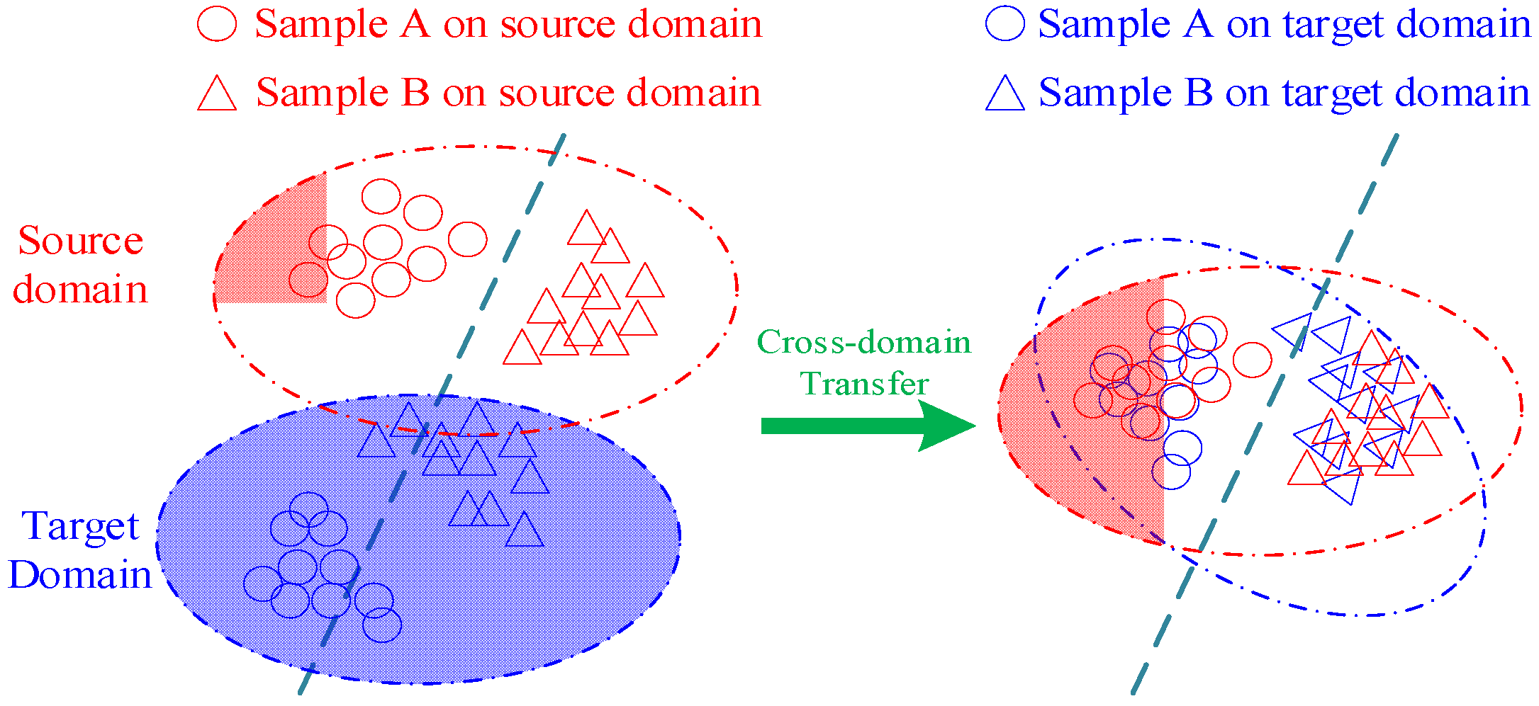
The domain adversarial adaptation [17] trains discriminators to make the distribution of data features consistent between different domains. As shown in Figure 1, the dashed line represents the category boundary, and the domain adaptation method maps features with different distributions to the same space, thereby reducing the distance between the two domains as much as possible. Domain Adversarial Neural Networks (DANNs) and Conditional Domain Adversarial Networks are neural network models used to address domain adaptation problems, leveraging unlabeled target domain data and achieving superior cross-domain fault diagnosis performance, and are widely applied in the fault diagnosis field. DANNs aim to reduce the data distribution difference between the source domain and the target domain by adversarially training the feature extractor and domain discriminator to learn domain-invariant features, thereby minimizing the marginal distribution difference between different domains. It outputs the probability distribution of fault categories through a label classifier and demonstrates good performance in domain adaptation tasks in fault diagnosis. However, this method fails to capture complex multimodal structure, even if the method successfully confuses the domain discriminator in adversarial training.

Figure 1.
Domain adversarial adaptive method based on transfer learning.
In contrast, the conditional domain adversarial networks method can utilize the discriminative information transmitted by the classifier to assist adversarial adaptation, thereby reducing the joint distribution difference in features and labels. The domain adversarial network introduces a Gradient Reversal Layer (GRL) in the network model, forming an adversarial relationship between the conditional domain discriminator and the feature extractor, and considers both marginal distribution and conditional distribution during domain alignment. The conditional adversarial loss and the prediction loss are defined as follows:
where represents the number of artificial fault samples (source domain), and represents the number of real industrial samples (target domain). and denote the distributions of the source and target domains, respectively. represents the combined distribution of all samples. is the feature extractor. is the conditional domain discriminator; is the classifier. represents the input samples. denotes the labels. The conditional adversarial loss ensures that the features extracted by are indistinguishable from the source, while the prediction loss ensures that the features extracted by are useful for the classification task.
3. Collaborative Domain Adversarial Network
3.1. Networking Framework
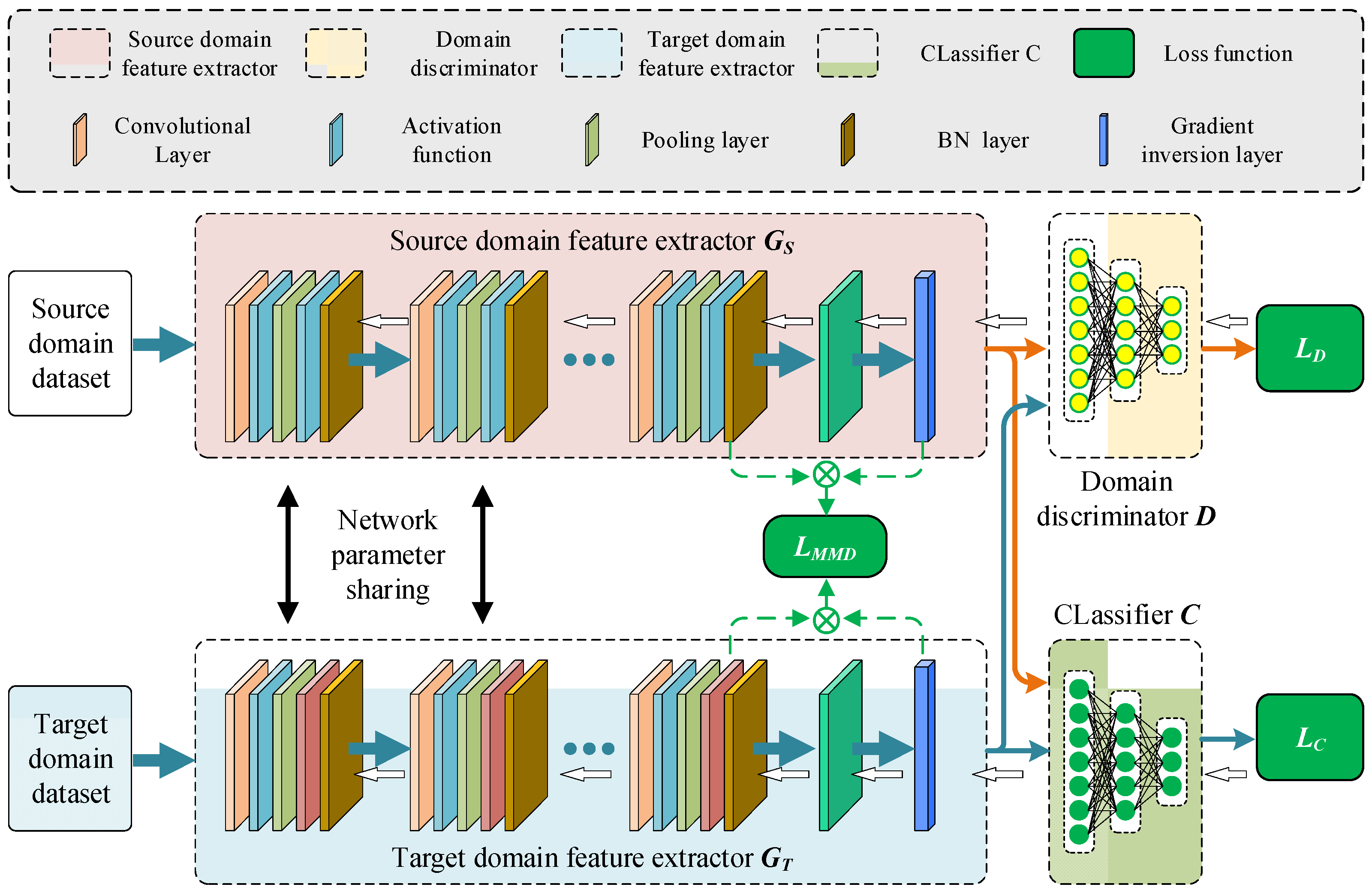
The deep domain adversarial transfer network structure is shown in Figure 2, which consists of two feature extractors and , a domain discriminator , and a classifier . The feature extractors and are used to extract features from the source domain samples and target domain samples, respectively. Traditional adversarial transfer networks only include one feature extractor, which is responsible for mapping both the features of samples in the source domain and target domain. Under such requirements, the performance of the feature extractor is greatly reduced. This study sets up two feature extractors for different tasks of mapping the source domain and target domain, so the feature mapping effect of the traditional transfer network is not as good as the proposed mapping effect. The feature extractors and are composed of convolutional layers (conv-layers), activation layers, normalization layers (BN), and max pooling layers (max-pool). The network parameters of the source domain feature extractor and the target domain feature extractor are represented by and , respectively, and the flattened output features are represented by and , respectively. A significant problem faced by the single-polar feature extractor of the traditional adversarial transfer network is that one set of network parameters must satisfy the mapping of both source domain samples and target domain samples, which may lead to differences in the feature distribution of the source domain and target domain mappings, resulting in negative transfer of samples and reduced fault classification accuracy. By constraining the feature mapping through two types of feature extractors, the network parameters of the feature extractor can be better optimized, and the consistency of the mapping distribution can be improved.

Figure 2.
Collaborative domain adversarial migration network framework.
The domain discriminator is used to identify the origin of the samples, with the output data type being Boolean. If the sample comes from the source domain, the domain discriminator outputs 0; if the sample comes from the target domain, the domain discriminator outputs 1. By constraining the distribution differences of different dimensional features between the source domain and the target domain through the domain discriminator , the network parameters of the domain discriminator are denoted by . The features extracted by the source domain and target domain feature extractors are flattened to obtain the source domain and target domain features and . The state classifier is used to identify the fault category of all samples, which consists of three fully connected layers (FCs) and two dropout layers. Since the purpose of the classifier is to identify different faults as accurately as possible based on the recognition features of the faults, it is necessary to reduce the loss of the label classifier on the data during the training process. Because the target samples are unlabeled, the state classifier is trained only using labeled source samples. The network structure and parameter settings of the feature extractors and , the domain discriminator and the classifier are shown in Table 1.

Table 1.
Model parameters of deep domain adversarial transfer network.
In the deep Domain Adversarial (DA) transfer neural network, max pooling was chosen to reduce the model’s sensitivity to time. The ReLU activation function is used after the convolutional layers, which can enhance the linear separability of the features. To better illustrate the proposed network, the meaning of the parameters in Table 1 is explained. For example, the convolutional network parameter in Table 1 represents the length of the kernel as 64, the depth of the kernel as 1, the number of kernels as 2, and the stride of the operation as 3; the network parameter of the max pooling layer represents taking the maximum value between two adjacent values, with a stride of 2; the network parameter of the FC layer represents the length of the input data of the upper FC layer as 1964, the output length as 64, and the number of network weight parameters is ; ReLU is the rectified linear unit; the last FC layer of the classifier is , where “k” represents the number of classification categories. Other network parameter meanings are similar. To extract features of different scales from the source domain and target domain samples, the feature extractors and are equipped with convolutional kernels of varying lengths. Longer kernels are used to extract low-dimensional sample features, medium-length convolutional kernels are used to extract intermediate-dimensional sample features, and shorter kernels are used to extract high-dimensional sample features.
3.2. Forward Propagation of Network Models
Firstly, define the input of the network model, and define the source domain and target domain samples as follows:
where ΨS_train, ΨT_train, and ΨT_test, respectively, represent the sets of source domain samples, the artificial fault samples in the laboratory used for training, and the real fault samples used for testing.
The samples in ΨT_train and ΨT_test are distinct. and denote artificial fault samples in the laboratory (source domain) and the real fault samples (target domain), respectively. nS, nT, and m represent the numbers of source domain samples, target domain training samples, and target domain testing samples. The forward propagation process of the DA network is illustrated in Figure 2, and the network parameters are defined as shown in Table 2.
Table 2.
Network module parameter definition.
The feature extractor operation in the network model is represented by GS (m = 1, 2, 3), the domain discriminator is represented by D, the state classifier is represented by D, and the flattening operation is represented by Flatten. The feature expressions of the fS and fT sets can be obtained as follows:
The obtained mapping features are input into the domain discriminator for sample source identification. The role of the domain discriminator is to distinguish the source of the samples as much as possible, that is, to identify the differences in features between the source domain samples and the target domain samples to the greatest extent possible, and then use them to train the feature extractor. The function of a feature extractor is to map the sample features of the source and target domains to the same distribution space as much as possible, reducing distribution differences. CDANs use Multi-Kernel Maximum Mean Discrepancies (MK-MMD) [29] to measure the distance between feature distributions and achieve the goal of predicting the labels of target domain samples. The loss calculation method of MK-MMD is as follows:
However, due to the lack of labels in the target domain data, the parameters of the last fully connected layer cannot be trained. To solve this issue, a pseudo-label learning strategy is introduced. The core idea of the pseudo-label strategy is to use the label with the highest predicted probability as the true label and to make the pseudo-label infinitely close to the true label through network iterative training. Laboratory samples and real samples are clustered, and pseudo-labels are created for real fault samples based on the probability of laboratory sample labels. The softmax function in the last layer calculates the probability distribution of the sample labels, and based on this probability distribution, it converts it into the final label of the sample. The label prediction method for target domain samples is as follows:
where is the fault label of the source domain sample , represents the set clustering range, and B represents Boolean operation, which means that if the sample features are mapped to the set clustering range, its value is taken as 1, and if they are not within the set clustering range, its value is taken as 0. K represents the number of all fault types. Using clustering to preliminarily predict the fault types of target domain samples and labeling them facilitates the training of a state classifier using target samples with predicted labels. The loss function of the discriminator is defined as follows:
In this equation, nS and nT represent the number of laboratory samples (source domain) and real samples (target domain), respectively. Here, di and dj denote the labels of domain for the laboratory samples and real samples. The domain label for a source sample is di = 0, while for a target sample it is dj = 1.
The mapped source domain feature is input into the state classifier C to obtain the predicted label for the sample. Since the real fault samples in this paper are unlabeled, only the source domain samples are used to train the state classifier C. The calculation formula for the state classifier C is defined as follows:
The state classifier uses the cross-entropy loss function, defined as follows:
The total loss function of the domain adversarial network is defined as follows [5]:
3.3. Network Parameter Optimization
The optimization objectives of the domain adversarial network model are as follows: (1) minimize the classification error between source domain and target domain samples; (2) minimize the domain discrepancy between sample distributions. The domain discriminator network parameters are optimized by maximizing the total loss function, while the feature extractor and state discriminator network parameters are , , and . They are optimized by minimizing the total loss function. The optimization process is defined as follows:
The domain adversarial network model adopts stochastic gradient descent (SGD) for network parameter optimization updates. The optimization method for network parameters is defined as follows:
The symbol μ denotes the learning rate for the classifier, while λ represents the learning rate for the feature extractor. The training process for network parameters is detailed in Table 2.
3.4. Fault Diagnosis Process
The optimization objectives of the CDAN are as follows: (1) minimize the identification error of fault samples; (2) minimize the inter-domain discrepancy of sample distributions.
Firstly, the original signals undergo preprocessing such as denoising, outlier removal, and completion. Then, the signals are segmented into source domain and target domain datasets using a signal sliding window approach. The data collected in the laboratory are defined as the source domain data, while the data from real industrial environments are defined as the target domain data. Comprehensive source domain data are collected in the laboratory, while a small amount of target domain data are collected in industrial environments. The second step involves updating and optimizing network parameters using the Stochastic Gradient Descent (SGD) backpropagation algorithm. According to Algorithm 1, the model parameters are iteratively updated to train the CDAN model and obtain the optimal network parameters. Finally, the unlabeled target domain fault samples (distinct from the target domain samples in the test data) are input into the optimized domain adversarial network model to predict fault types. The model’s performance is assessed by calculating the predicted fault diagnosis accuracy. The formula for predicting bearing fault types is as follows:
where max(·) extracts the label with the highest fault probability.
| Algorithm 1. Domain adversarial network training process | |||||||
| Input | Labeled source domain dataset , unlabeled target domain dataset , learning , μ. | ||||||
| 1: | Initialize the all network parameters. | ||||||
| 2: | for do | ||||||
| 3: | for do | ||||||
| 4: | for not reaching Nash equilibrium do | ||||||
| 5: | Forward propagation: | ||||||
| 6: | Calculate the features fS and fT using Formula (6); | ||||||
| 7: | Calculate the features LD using Formula (10); | ||||||
| 8: | Calculate the features LC using Formula (13); | ||||||
| 9: | Network parameter optimization: | ||||||
| 10: | Calculate the features using Formula (15); | ||||||
| 11: | Calculate the features using Formula (16); | ||||||
| 12: | end | ||||||
| 13: | Update parameters by Formula (18) to (21) | ||||||
| 14: | end | ||||||
| 15: | end | ||||||
| Output: | Optimal network parameters: ; | ||||||
4. Experimental Verification and Analysis
This paper uses the bearing fault datasets [30] from the Case Western Reserve University (CWRU) electrical engineering laboratory in the United States and Paderborn University (PU) in Germany [31] to experimentally validate the advanced and effective nature of the CDAN.
4.1. Dataset Description
4.1.1. CWRU Dataset
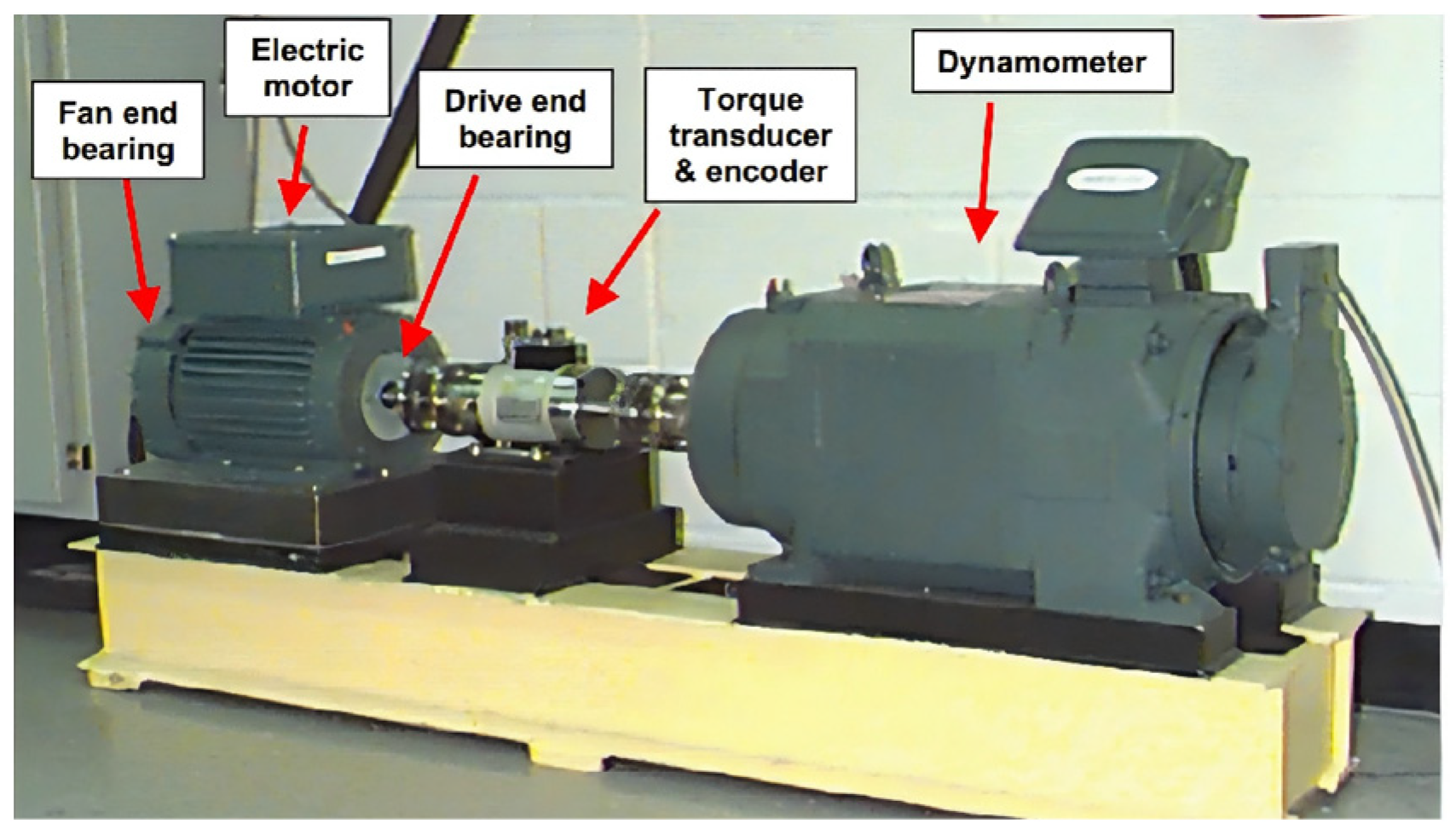
The evaluation was conducted on the CWRU dataset [30], where the bearing experimental system at CWRU is depicted in Figure 3. Single-point defects of specified diameters were introduced on the drive end and fan end bearings (6205-2RSJEM SKF deep groove ball bearings, SKF, Gothenburg, Sweden) and the rolling elements.

Figure 3.
The bearing experimental system of CWRU [30].
In this study, we focused primarily on defects 7, 14, and 21 milli-inch in diameter, as their vibration signals are relatively small compared to defects of larger diameters. Therefore, our experiments included four bearing conditions: Healthy (H), Ball Fault (BF), Outer Race Fault (OF), and Inner Race Fault (IF). Data collection was conducted under four load conditions (0, 1, 2, 3 hp), corresponding to motor speeds of 1797, 1772, 1750, and 1730 revolutions per minute (r/min). This study designed a total of 10 fault categories, detailed in Table 3.
Table 3.
Classification of fault types in CWRU dataset.
For each fault class, 500 samples were randomly selected from the original signal data. Each sample consisted of amplitude signals containing 2048 data points. In industrial scenarios, vibration signals often exhibit different characteristic distributions due to varying operating conditions and environments. This variability can degrade the performance of models trained in a supervised manner on signals collected under different operating conditions. Therefore, unsupervised domain adaptation models are highly useful and necessary in different settings.
As shown in Table 4, labels A to F represent different operating conditions, defining data from the drive end as the source domain data and data from the fan end as the target domain data. Domain adaptation tasks are denoted as A→D, B→E, C→F, D→A, E→B, and F→C. Taking experiment A→D as an example, this means training the model under condition A (source domain, drive end, 1 hp load) and transferring it to condition D (target domain, drive end, 2 hp load).
Table 4.
CWRU dataset working condition settings.
4.1.2. PU Dataset
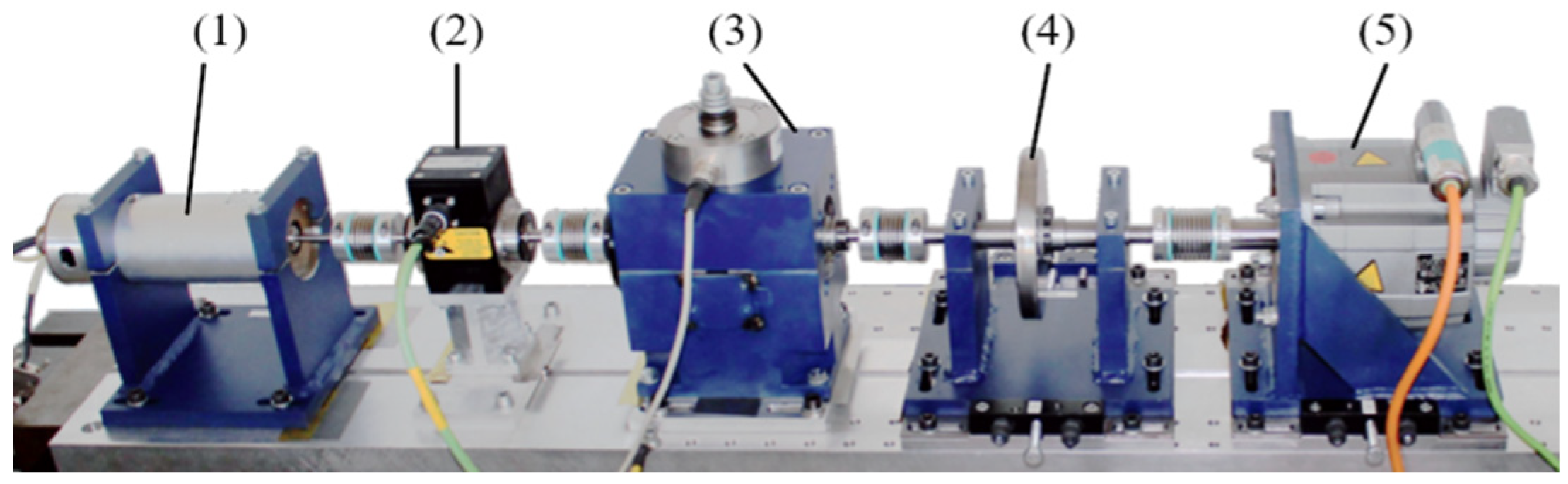
The Paderborn University (PU) experimental setup is illustrated in Figure 4. The setup consists of an electric motor (1), torque measurement shaft (2), rolling bearing test module (3), flywheel (4), and load motor (5). The bearing data in the PU dataset corresponds to three bearing conditions: outer race fault (OF), inner race fault (IF), and normal (N).

Figure 4.
Paderburn University experimental platform [32].
Some bearing faults were artificially created through discharge machining, while others occurred naturally over extended operational periods. There are four operating conditions (labeled as A, B, C, D) with different speeds and load torques, detailed in Table 5.
Table 5.
PU dataset working condition settings.
Based on the causes of different bearing faults, the PU bearing dataset is categorized into eight distinct classes, as shown in Table 6. For each class, 500 data samples were randomly extracted from the original vibration signals under various operating conditions, with each sample length set to 2048. Domain adaptation tasks for the PU bearing dataset were conducted under different operating conditions, denoted as A→B, B→C, C→D, and D→A.
Table 6.
Classification of fault types in PU dataset.
4.2. Comparison Methods
This study validates the performance of the CDAN by comparing it with four advanced fault diagnosis methods. The four comparison methods are described as follows.
Model 1: The fault diagnosis technology based on deep learning requires a large number of labeled datasets. However, considering different operating conditions, it is impractical to obtain labeled datasets for each operating condition. To address this issue, Kim et al. [32] proposed a diagnostic method for unlabeled data by combining clustering and domain adaptation.
Model 2: Long et al. [29] proposed a multi-linear mapping method for sample labels in order to learn more fault features from source domain samples and target domain samples to improve the accuracy of fault recognition.
Model 3: Ganin et al. [18] proposed a new DA representation learning model by proposing a neural network. The model uses an extractor to map features from the source and target domains. In contrast, the model proposed in this paper sets different feature extractors for mapping source domain samples and target domain samples separately.
Model 4: Zhang et al. [33] addressed the issue of decreased diagnostic accuracy due to distribution differences in bearing data under different operating conditions.
All models were run on a computer equipped with an Intel Core i9-9900K processor, NVIDIA GeForce RTX 2080Ti GPU, and 128 GB of RAM. The computing environment included Windows 10 operating system, Python 3.8, and PyTorch 1.11.0. All comparison models used SGD with momentum for backpropagation to update network parameters. The iteration period was set to 100, the learning rate to 10−4 and the batch size to 100. Equal amounts of data from the laboratory and real working conditions were used in each batch. All models were trained until the loss function reached a relatively stable value.
4.3. Experimental Results and Analysis
4.3.1. Results and Analysis on CWRU Dataset
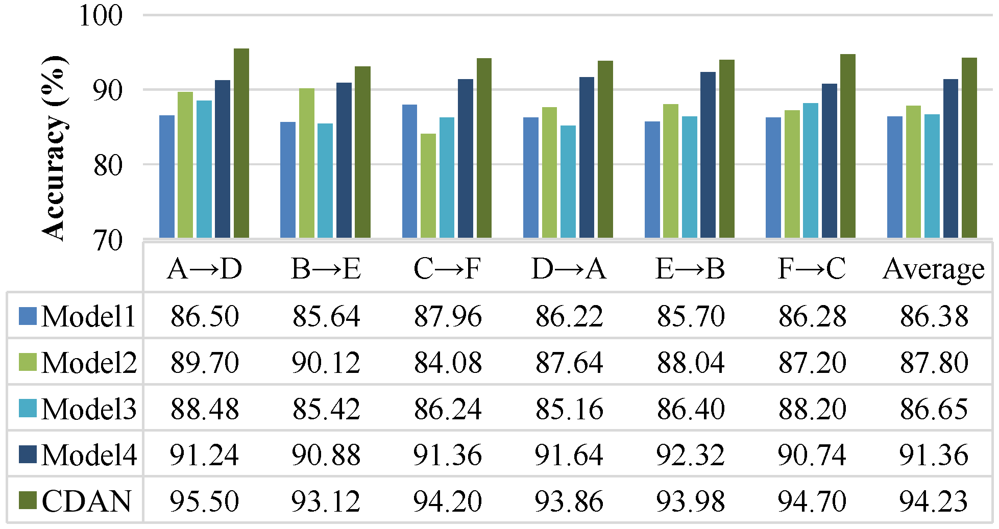
The experimental results on the CWRU dataset are shown in Figure 5. The average training time for the CDAN was 12.67 s, while the average training time for Models 1 to 4 was 30.65 s, 27.81 s, 19.27 s, and 16.89 s, respectively. The average accuracy of fault diagnosis for the comparison methods was 86.38%, 87.80%, 86.64%, and 91.36% respectively. The CDAN achieved an average fault diagnosis accuracy of 94.22%, which is more than 6% higher than Model 1, Model 2, and Model 3, and 2.86% higher than Model 4. Model 3 used an extractor to map features from both source and target domains, while the model proposed in this paper separately set different feature extractors for mapping laboratory samples and real fault samples. The CDAN achieved a fault diagnosis average accuracy 7.85% higher than Model 3, indicating that a model with two feature extractors performs significantly better in recognition performance than a single feature extractor.
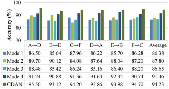
Figure 5.
Experimental results on the CWRU dataset.
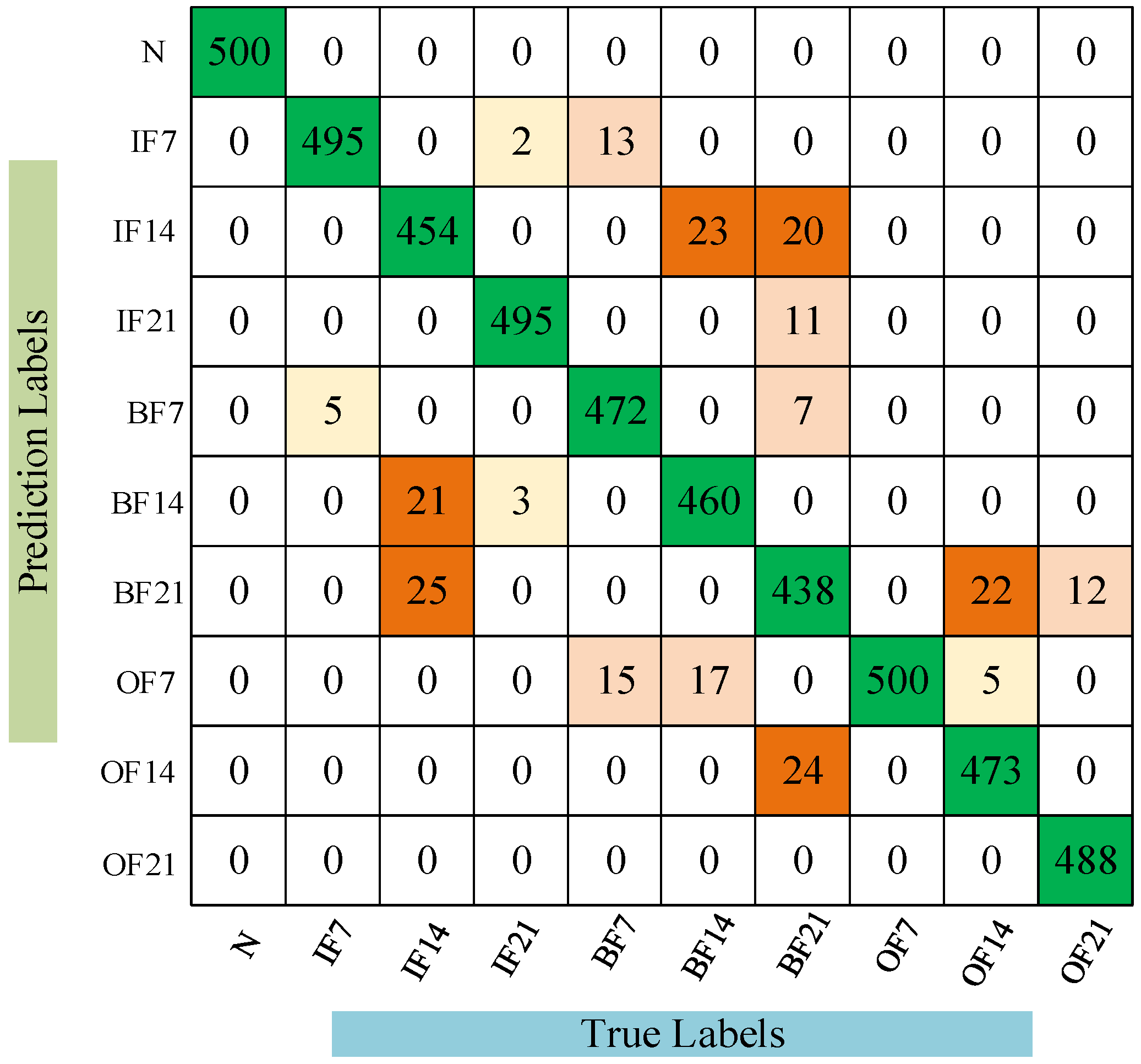
To better understand the cross-domain diagnostic performance of the CDAN, confusion matrices of the models under the A→D operating conditions are presented to further elucidate the recognition results for specific fault patterns, as shown in Figure 6. It is clear that CDAN can effectively detect the health status of bearings across six different cross-domain scenarios. The comparative results of the experiment show that the CDAN has good recognition ability for unlabeled bearing faults. Multiple sets of experimental data are superior to the compared methods, indicating that CDAN has better generalization performance and stability.
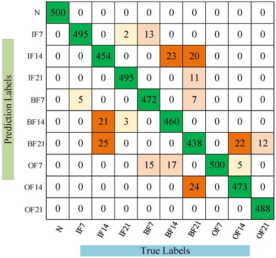
Figure 6.
Confusion matrix of CDAN under conditions A→D.
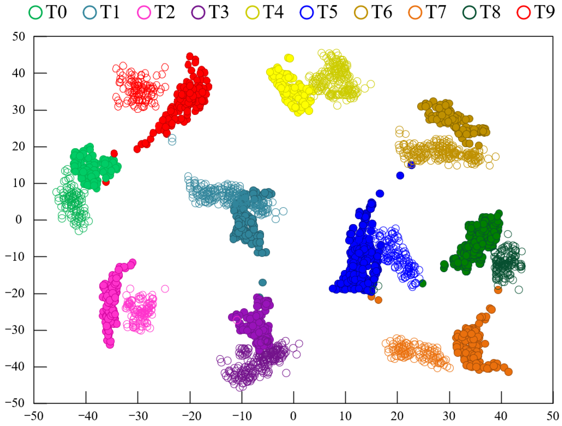
To explore the advantages of using two types of feature extractors for mapping, the t-distributed Stochastic Neighborhood Embedding (t-SNE) method [34] was employed to visualize the features during the data transfer process. The feature visualization results using the CDAN method under experimental conditions A→D are shown in Figure 7, while Figure 8 displays the feature visualization results using the Model 3 method under experimental conditions A→D. A comparison between Figure 7 and Figure 8 clearly shows that the clustering of samples from the same fault category in Figure 7 is more compact, with larger distances between fault category centers, indicating better performance compared to Figure 8. This demonstrates that the proposed model’s fault recognition performance is superior to that of Model 3.
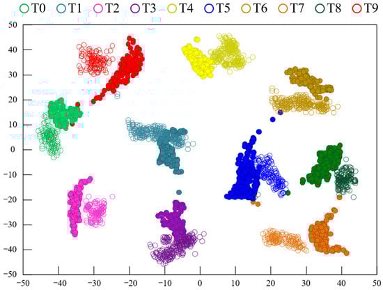
Figure 7.
Feature clustering diagram of CDAN on the CWRU dataset.
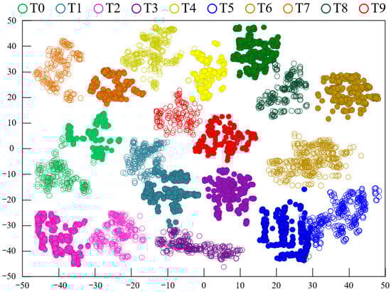
Figure 8.
Feature clustering diagram of Model 3.
4.3.2. Results and Analysis on PU Dataset
The fault size categories of the samples in the PU dataset are fewer than those in the CWRU dataset, but their fault categories are diverse, and the real bearing faults in this domain are closer. The fault recognition accuracy of the CDAN and four comparison methods on the PU dataset is shown in Figure 9. The average training time for the CDAN was 14.43 s, while the average training time for Models 1 to 4 was 36.89 s, 31.64 s, 23.08 s, and 18.90 s, respectively. On the PU dataset, the average accuracy of fault diagnosis for the comparison methods was 82.32%, 84.88%, 84.56%, and 85.69% respectively. The CDAN achieved an average fault diagnosis accuracy of 89.78%, which is more than 4% higher than Model 1, Model 2, Model 3, and Model 4. Model 3 used an extractor to map features from both laboratory and real fault samples, while the model proposed in this paper separately set different feature extractors for mapping laboratory and real fault samples. The CDAN achieved an average fault diagnosis accuracy 5.22% higher than Model 3, indicating that a model with two feature extractors performs significantly better in recognition performance than a single feature extractor.
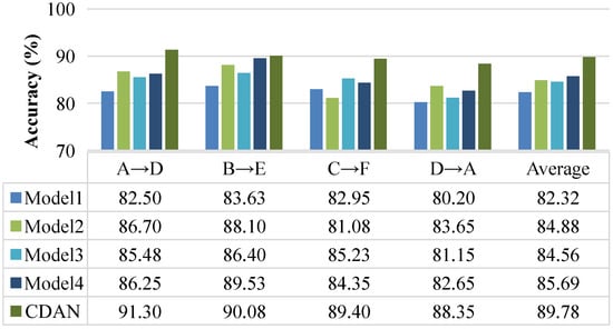
Figure 9.
Experimental results on the PU dataset.
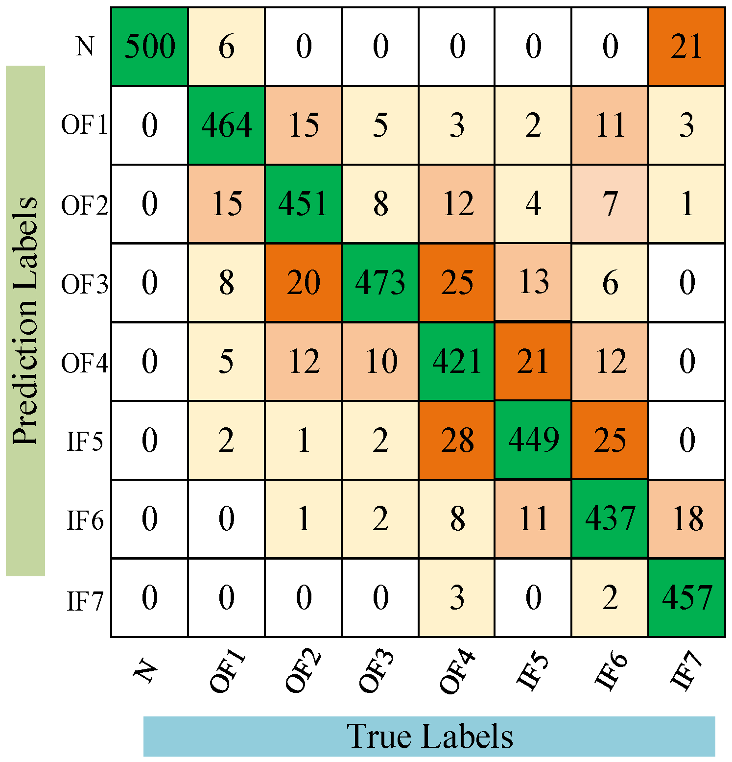
In order to explore the details of CDAN in diagnosing unlabeled bearing faults, the confusion matrix of fault identification results under A→B operating conditions is shown in Figure 10.
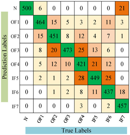
Figure 10.
Confusion matrix of CDAN under condition A→B.
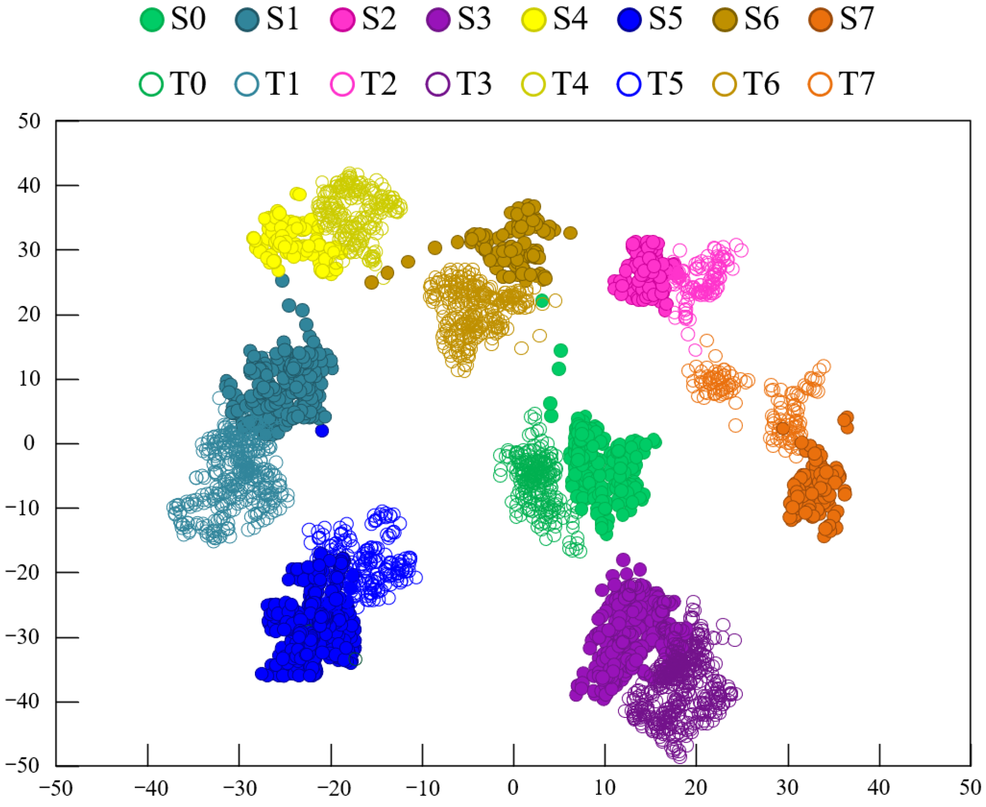
It is clear that the CDAN can effectively detect the health status of bearings across four different cross-domain scenarios. The comparative results of the experiment show that the CDAN has good recognition ability for unlabeled bearing faults. Multiple sets of experimental data are superior to the compared methods, indicating that the CDAN has better generalization performance and stability. The feature visualization results using the CDAN method under experimental conditions A→B are shown in Figure 11, while Figure 12 displays the feature visualization results using the Model 3 method under experimental conditions A→B. A comparison between Figure 11 and Figure 12 clearly shows that the clustering of samples from the same fault category in Figure 11 is more compact, with larger distances between different fault categories, indicating better performance compared to Figure 12. This demonstrates that the proposed model’s fault recognition performance surpasses that of Model 3.

Figure 11.
Feature clustering diagram of CDAN on the PU dataset.
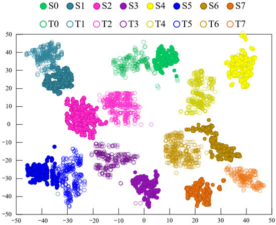
Figure 12.
Feature clustering diagram of Model 3.
5. Conclusions
The proposed CDAN aims to solve the negative transfer problem in transfer learning based fault diagnosis models and improve the accuracy of unlabeled bearing fault diagnosis. By employing two types of feature extractors and multi-linear mapping, the classifier’s predicted classification information is fed back to the domain discriminator to enhance the learning of domain-invariant features. To validate the feasibility of this model, experiments were conducted on two datasets. On the CRWU dataset, data under different loads and positions were respectively set as source domain and target domain datasets, verifying the superiority and stability of the CDAN. Similar results were observed on the PU dataset. Using t-SNE, the visualization of classification features learned by different models shows that the CDAN clustering has good intra-class and inter-class compactness. Compared with four other advanced methods, the CDAN improved the average recognition accuracy by 7.85% and 5.22%, respectively. This indirectly proves the effectiveness and superiority of the CDAN in identifying unlabeled bearing faults. The CDAN can be applied for fault diagnosis of supporting bearings in motors. Further research is needed to determine whether it can be used for fault diagnosis of rotors, coils, and other components in motors. These results indicate that the CDAN effectively reduces cross-domain distribution discrepancies in sample transfer learning and is a promising method for rolling bearing fault diagnosis. CDAN requires sufficient laboratory failure samples as support, which requires a lot of manpower and resources. The generation of fault data through digital twins can perfectly solve this problem, which is also the future research direction of this study.
Author Contributions
Conceptualization, Y.W. and Z.Z.; methodology, Y.W. and Z.Z.; software, C.X. and X.L.; resources, Y.W. and Z.Z.; writing—original draft preparation, Y.W. and Z.Z.; writing—review and editing, Y.W. and Z.Z.; project administration, L.W. All authors have read and agreed to the published version of the manuscript.
Funding
This research was funded by the Open Fund of State Key Laboratory of Coal Mine Disaster Prevention and Control (2022SKLKF14, 2022SKLKF07), the China Postdoctoral Science Foundation (2024M753655), the Ministry of Industry and Information Technology Project under Grant 167; the Independent Key Project of Intelligent Collaborative Innovation Center of China Coal Technology and Engineering Group Chongqing Research Institute under Grant 2023ZDZX04, the Innovative Research Group of Universities in Chongqing (CXQT21024), the Science and Technology Research Plan Project (KJQN202200835),and the Scientific Research Startup Project for High-Level Talents (No. 2256013).
Institutional Review Board Statement
Not applicable.
Informed Consent Statement
Not applicable.
Data Availability Statement
The original contributions presented in the study are included in the article, further inquiries can be directed to the corresponding author.
Conflicts of Interest
Authors Zhigang Zhang, Chunrong Xue, Xiaobo Li and Yinjun Wang were employed by the company China Coal Technology and Engineering Group Corp Chongqing Research Institute. The remaining authors declare that the research was conducted in the absence of any commercial or financial relationships that could be construed as a potential conflict of interest.
References
- Wang, Y.; Ding, X.; Zeng, Q.; Wang, L.; Shao, Y. Intelligent Rolling Bearing Fault Diagnosis via Vision ConvNet. IEEE Sens. J. 2021, 21, 6600–6609. [Google Scholar] [CrossRef]
- Wang, Y.; Ding, X.; Liu, R.; Shao, Y. ConditionSenseNet: A Deep Interpolatory ConvNet for Bearing Intelligent Diagnosis Under Variational Working Conditions. IEEE Trans. Ind. Inform. 2022, 18, 6558–6568. [Google Scholar] [CrossRef]
- Zhang, S.; Wang, B.; Habetler, T.G. Deep Learning Algorithms for Bearing Fault Diagnostics-A Comprehensive Review. IEEE Access 2020, 8, 29857–29881. [Google Scholar] [CrossRef]
- Zhao, R.; Yan, R.; Chen, Z.; Mao, K.; Wang, P.; Gao, R.X. Deep learning and its applications to machine health monitoring. Mech. Syst. Signal Process. 2019, 115, 213–237. [Google Scholar] [CrossRef]
- Liu, G.; Zhang, C.; Xu, S.; Zhang, J.; Wu, L. A New Lightweight Fault Diagnosis Framework Towards Variable Speed Rolling Bearings. IEEE Access 2024, 12, 70170–70183. [Google Scholar] [CrossRef]
- Chang, Y.; Bao, G. Enhancing Rolling Bearing Fault Diagnosis in Motors Using the OCSSA-VMD-CNN-BiLSTM Model: A Novel Approach for Fast and Accurate Identification. IEEE Access 2024, 12, 78463–78479. [Google Scholar] [CrossRef]
- Yang, J.; Xie, G.; Yang, Y. Fault Diagnosis of Rotating Machinery Using Denoising-Integrated Sparse Autoencoder Based Health State Classification. IEEE Access 2023, 11, 15174–15183. [Google Scholar] [CrossRef]
- Huo, C.; Jiang, Q.; Shen, Y.; Lin, X.; Zhu, Q.; Zhang, Q. A class-level matching unsupervised transfer learning network for rolling bearing fault diagnosis under various working conditions. Appl. Soft Comput. 2023, 146, 110739. [Google Scholar] [CrossRef]
- Wen, L.; Yang, G.; Hu, L.; Yang, C.; Feng, K. A new unsupervised health index estimation method for bearings early fault detection based on Gaussian mixture model. Eng. Appl. Artif. Intell. 2024, 128, 107562. [Google Scholar] [CrossRef]
- Brito, L.C.; Susto, G.A.; Brito, J.N.; Duarte, M.A.V. Fault Diagnosis using eXplainable AI: A transfer learning-based approach for rotating machinery exploiting augmented synthetic data. Expert Syst. Appl. 2023, 232, 120860. [Google Scholar] [CrossRef]
- Lu, W.; Liang, B.; Cheng, Y.; Meng, D.; Yang, J.; Zhang, T. Deep model based domain adaptation for fault diagnosis. IEEE Trans. Ind. Electron. 2016, 64, 2296–2305. [Google Scholar] [CrossRef]
- Li, X.; Hu, Y.; Zheng, J.; Li, M.; Ma, W. Central moment discrepancy based domain adaptation for intelligent bearing fault diagnosis. Neurocomputing 2021, 429, 12–24. [Google Scholar] [CrossRef]
- Zmarzły, P. Influence of Bearing Raceway Surface Topography on the Level of Generated Vibration as an Example of Operational Heredity. Indian J. Eng. Mater. Sci. 2020, 27, 356–364. [Google Scholar]
- Liu, Z.-H.; Lu, B.-L.; Wei, H.-L.; Chen, L.; Li, X.-H.; Rätsch, M. Deep adversarial domain adaptation model for bearing fault diagnosis. IEEE Trans. Syst. Man Cybern. Syst. 2021, 51, 4217–4226. [Google Scholar] [CrossRef]
- Jiao, J.; Lin, J.; Zhao, M.; Liang, K.; Ding, C. Cycle-consistent adversarial adaptation network and its application to machine fault diagnosis. Neural Netw. 2022, 145, 331–341. [Google Scholar] [CrossRef]
- Li, Y.; Song, Y.; Jia, L.; Gao, S.; Li, Q.; Qiu, M. Intelligent fault diagnosis by fusing domain adversarial training and maximum mean discrepancy via ensemble learning. IEEE Trans. Ind. Informat. 2021, 17, 2833–2841. [Google Scholar] [CrossRef]
- Huang, Z.; Lei, Z.; Wen, G.; Huang, X.; Zhou, H.; Yan, R.; Chen, X. A multisource dense adaptation adversarial network for fault diagnosis of machinery. IEEE Trans. Ind. Electron. 2022, 69, 6298–6307. [Google Scholar] [CrossRef]
- Ganin, Y.; Ustinova, E.; Ajakan, H.; Germain, P.; Larochelle, H.; Laviolette, F.; Marchand, M.; Lempitsky, V. Domain-adversarial training of neural networks. In Domain Adaptation in Computer Vision Applications; Csurka, G., Ed.; Springer International Publishing AG: Cham, Switzerland, 2017; pp. 189–209. [Google Scholar]
- Feng, L.; Zhao, C. Fault Description Based Attribute Transfer for Zero-Sample Industrial Fault Diagnosis. IEEE Trans. Ind. Inform. 2021, 17, 1852–1862. [Google Scholar] [CrossRef]
- Shen, C.; Wang, X.; Wang, D.; Li, Y.; Zhu, J.; Gong, M. Dynamic Joint Distribution Alignment Network for Bearing Fault Diagnosis Under Variable Working Conditions. IEEE Trans. Instrum. Meas. 2021, 70, 3510813. [Google Scholar] [CrossRef]
- Xu, D.; Li, Y.; Song, Y.; Jia, L.; Liu, Y. IFDS: An Intelligent Fault Diagnosis System with Multisource Unsupervised Domain Adaptation for Different Working Conditions. IEEE Trans. Instrum. Meas. 2021, 70, 3526510. [Google Scholar] [CrossRef]
- Li, X.; Liu, S.; Xiang, J.; Sun, R. A transfer learning strategy based on numerical simulation driving 1D Cycle-GAN for bearing fault diagnosis. Inf. Sci. 2023, 642, 119175. [Google Scholar] [CrossRef]
- Ragab, M.; Chen, Z.; Wu, M.; Li, H.; Kwoh, C.-K.; Yan, R.; Li, X. Adversarial multiple-target domain adaptation for fault classification. IEEE Trans. Instrum. Meas. 2021, 70, 3500211. [Google Scholar] [CrossRef]
- Deng, M.; Deng, A.; Shi, Y.; Xu, M. Correlation regularized conditional adversarial adaptation for multi-target-domain fault diagnosis. IEEE Trans. Ind. Inform. 2022, 18, 8692–8702. [Google Scholar] [CrossRef]
- Zhao, M.; Zhong, S.; Fu, X.; Tang, B.; Pecht, M. Deep Residual Shrinkage Networks for Fault Diagnosis. IEEE Trans. Ind. Inform. 2020, 16, 4681–4690. [Google Scholar] [CrossRef]
- Shao, J.; Huang, Z.; Zhu, J. Transfer Learning Method Based on Adversarial Domain Adaption for Bearing Fault Diagnosis. IEEE Access 2020, 8, 119421–119430. [Google Scholar] [CrossRef]
- Li, B.; Tang, B.; Deng, L.; Wei, J. Joint attention feature transfer network for gearbox fault diagnosis with imbalanced data. Mech. Syst. Signal Process. 2022, 176, 109146. [Google Scholar] [CrossRef]
- Wang, C.; Chen, D.; Chen, J.; Laid, X.; He, T. Deep regression adaptation networks with model-based transfer learning for dynamic load identification in the frequency domain. Eng. Appl. Artif. Intell. 2021, 102, 104244. [Google Scholar] [CrossRef]
- Long, M.; Cao, Y.; Wang, J.; Jordan, M.I. Learning transferable features with deep adaptation networks. arXiv 2015, arXiv:1502.02791v2. [Google Scholar]
- Bearing Data Center. Available online: https://gitcode.com/open-source-toolkit/5848e/ (accessed on 7 September 2024).
- Lessmeier, C.; Kimotho, J.K.; Zimmer, D.; Sextro, W. Condition monitoring of bearing damage in electromechanical drive systems by using motor current signals of electric motors: A benchmark data set for data-driven classification. Proc. PHM Soc. Eur. Conf. 2016, 3, 1–17. [Google Scholar] [CrossRef]
- Kim, T.; Lee, S. A Novel Unsupervised Clustering and Domain Adaptation Framework for Rotating Machinery Fault Diagnosis. IEEE Trans. Ind. Inform. 2023, 19, 9404–9412. [Google Scholar] [CrossRef]
- Zhang, Z.; Yang, Q. Unsupervised feature learning with reconstruction sparse filtering for intelligent fault diagnosis of rotating machinery. Appl. Soft Comput. 2022, 115, 108207. [Google Scholar] [CrossRef]
- Van Der Maaten, L.; Hinton, G. Visualizing data using t-SNE. J. Mach. Learn. Res. 2008, 9, 2579–2625. [Google Scholar]


Disclaimer/Publisher’s Note: The statements, opinions and data contained in all publications are solely those of the individual author(s) and contributor(s) and not of MDPI and/or the editor(s). MDPI and/or the editor(s) disclaim responsibility for any injury to people or property resulting from any ideas, methods, instructions or products referred to in the content. |
© 2024 by the authors. Licensee MDPI, Basel, Switzerland. This article is an open access article distributed under the terms and conditions of the Creative Commons Attribution (CC BY) license (https://creativecommons.org/licenses/by/4.0/).