Accurate Prediction of Dissolved Oxygen in Perch Aquaculture Water by DE-GWO-SVR Hybrid Optimization Model

Abstract

In order to realize the accurate and reliable prediction of the change trend of dissolved oxygen (DO) content in California perch aquaculture water, this paper proposes a second-order hybrid optimization support vector machine (SVR) model based on Differential Evolution (DE) and Gray Wolf Optimizer (GWO), shortened to DE-GWO-SVR, to predict the DO content with the characteristics of nonlinear and non-smooth water quality data. Experimentally, data for the water quality, including pH, water temperature, conductivity, salinity, total dissolved solids, and DO, were collected. Pearson’s correlation coefficient (PPMCC) was applied to explore the correlation between each water quality parameter and DO content. The optimal DE-GWO-SVR model was established and compared with models based on SVR, back-propagation neural network (BPNN), and their optimization models. The results show that the DE-GWO-SVR model proposed in this paper can effectively realize the nonlinear prediction and global optimization performance. Its R², MSE, MAE and RMSE can be up to 0.94, 0.108, 0.2629, and 0.3293, respectively, which is better than those of other models. This research provides guidance for the efficient prediction of DO in perch aquaculture water bodies for increasing the aquaculture effectiveness and reducing the aquaculture risk, providing a new exploratory path for water quality monitoring.

1. Introduction

Aquaculture is an important part of the fishery industry, and the quality of the aquaculture water directly affects the aquatic environment, yield and quality of aquatic products [1]. Currently China’s aquaculture industry is still at the stage of rough development, fishery facilities and equipment and water quality management technology are relatively backward. Aquaculture water as an open, dynamic, variable and complex system, water quality is easily affected by many factors such as physical, chemical, biological and human activities [2]. According to statistics, the annual aquaculture economic loss caused by deterioration of aquaculture water quality in China is about 15 billion yuan [3]. Among them, the dissolved oxygen (DO) content in aquaculture water is one of the key factors for the survival of fish, which has an important impact on the feed consumption, energy consumption and metabolic rate of fish [4]. If the DO level is lower than 3 mg/L, it can easily lead to fish diseases and a large number of deaths [5]. In addition, the DO level in aquaculture is one of the most important parameters in water quality management [1]. The core issue for water quality DO management is to estimate future changes in the spatial and temporal patterns and development trends of water quality DO based on the monitored historical data, so as to provide a decision-making basis for preventing further deterioration of aquaculture water quality, realizing early warning and formulating water quality control measures [6]. Therefore, it is of great practical significance to carry out research on water quality DO prediction to promote scientific management of water quality and reduce aquaculture risk [7,8].

At present, the research on the prediction method of DO content in aquaculture water quality has become a hotspot in the field of aquaculture, and the Internet of Things (IoT) technology, which is centered on online sensors, has made great progress in water quality monitoring applications [9]. However, due to such factors as easy equipment failure and human interference, the collected data suffer loss, invalidity, and noise interference, resulting in a lack of comprehensiveness and systematism of water quality samples [10]. Therefore, the Internet of Things technology is still in its infancy in the DO prediction of water quality. Usually, it can only carry out real-time monitoring and simple regulation of water quality and meteorological data through sensors, which prevents achieving accurate online prediction [11,12]. In addition, because the water environment is a mixed system with multiple factors coexisting, in practical application the prediction of water quality DO content will be affected by the changes of many factors, such as ambient temperature, ambient air pressure, water depth, water temperature, wind speed, PH, and other factors in time and space, which may result in the abnormality of the predicted data [13,14]. Therefore, in the prediction of water quality DO content, each environmental factor can be used as an independent variable to eliminate the randomness, synergistic phenomenon and coherent effect among the variables, and the algorithm can be used to establish a predictive model based on multiple independent variables, thus increasing the accuracy, reliability, and robustness of the prediction result [15].

In recent years, with the high-speed development of modern intelligent computing methods, domestic and foreign scholars have studied the use of existing real-time monitoring information of Internet of Things (IoT), big data analysis, artificial intelligence algorithms to solve problems related to the prediction of water quality DO. These DO prediction models can be summarized as: (1) the ecological dynamics model, based on traditional prediction methods such as the water quality simulation method, gray prediction, time-series analysis, and multiple regressions, etc.; (2) the empirical intelligence model, based on prediction methods such as the genetic algorithm, support vector machine, neural network, ant colony optimization, etc.; (3) the cluster intelligence combination model, based on multi-model mixing [16,17]. At present, the combination model is a hot spot in the research of water quality prediction. Scholars have carried out much research on this topic, and have put forward a variety of combination prediction methods. Jiang et al. [18] used Monte Carlo simulation (MCS) to assess the risk of COD pollution in a river section, and introduced an artificial neural network (ANN) to improve the computational efficiency of the traditional method. Kadam et al. [19] used a combination of the ANN and multivariate linear Regression (MLR) methods to predict the suitability of groundwater quality data, and experiments showed that the ANN model outperformed the traditional MLR model. Abyaneh et al. [20] attempted to use the model to predict the Chemical Oxygen Demand (COD) and Biological Oxygen Demand (BOD) in the wastewater water body by finding the optimized topological model of ANN and achieved a better prediction result. However, the water quality prediction model mentioned above has problems, such as the uncertainty of preset parameters, single model, and no preprocessing of data. Khan et al. [21] used principal component regression (PCR) to extract the water quality index (WQI), and then fused it with gradient-enhanced regression (GBR) to form the PCR-GBR regressor, which provides a new idea for the prediction of water quality parameters. Xu et al. [22] combined wavelet transforms (WT) with multiple machine learning models to explore the feasibility of the hybrid models for water quality dissolved oxygen prediction, and concluded that the multicomponent framework improved the prediction accuracy of the stand-alone model to a certain extent. Li et al. [23] introduced sparse self-encoder (SAE) on the basis of a long-short-story memory neural network (LSTM) to compose the SAE-LSTM model; the model pre-training by SAE was completed to initialize the network parameters, and satisfactory prediction results were achieved. Li et al. [24] proved the feasibility of the GRU model in water quality prediction by introducing the gated recurrent unit (GRU) model and comparing it with the LSTM and the recurrent neural network (RNN) model. Guo et al. [25] introduced the Pathfinder Algorithm (PFA) for seeking parameter optimization of the GRU and combined it with the PCA algorithm to form the PCA-PFA-GRU model, which achieved satisfactory accuracy in the prediction of water quality dissolved oxygen. Su et al. [8] improved the Sparrow Search Algorithm (SSA) through the introduction of Skew-Tent mapping and combined it with the Support Vector Machines (SVM) model and the ISSA-SVR model was finally formed for the study of water quality prediction models. Huang et al. [26] introduced complete empirical modal decomposition (CEEMDAN-LZC) to decompose the dissolved oxygen time series, reconstructed the new features, and then used the particle swarm optimization algorithm (PSO) to optimize the combination of the GRU model, which provided a reliable prediction of the DO content in aquaculture support. The above study shows that the combined model has the advantages of mining more useful information and improving the convergence speed and prediction accuracy, which provides a new direction for the prediction of the DO content in water quality, but the method of determining the combined weight coefficients and the optimization method need to be further studied.

The machine learning method in artificial intelligence technology is the frontier of the research on DO prediction model of aquaculture water quality, and the machine learning method represented by SVR is able to characterize the water quality factors with multivariate, coupling, and nonlinearity, and can avoid the limitations of small samples, high dimensionality, overfitting, and local extremes of the traditional method, which has achieved a better application in the research of the DO content prediction in water quality [27]. In addition, the SVR-based cluster intelligent combination model is also an important research direction for the prediction method of DO in aquaculture water quality, but the choice of parameter combination optimization still lacks theoretical guidance [28]. Compared with the traditional genetic algorithm, ant colony algorithm, particle swarm algorithm, and other swarm intelligent optimization algorithms, the Differential Evolution (DE) and Gray Wolf Optimizer (GWO), as new swarm intelligent optimization algorithms, have the advantages of finding the global optimal solution in multi-dimensional space and dynamically adjusting the parameter weights adaptively. It has a broad application prospect in constrained optimization, cluster optimization, nonlinear optimization, continuous optimization, and combinatorial optimization [29,30]. The combined prediction method, based on the cluster intelligent optimization algorithm and SVR model, can better meet the demand for the accurate prediction of water quality DO content by using the complementary effect, which is an important research direction and an inevitable development trend for online water quality control in the aquaculture field.

Therefore, this paper proposes a cluster intelligent combination model based on DE-GWO-SVR, which first uses the Pearson’s correlation coefficient (PPMCC) to preprocess the water quality data of perch aquaculture, and then uses the DE algorithm to adaptively adjust the variation and evolution of the population in the GWO algorithm, so that the GWO algorithm is able to jump out of the trap of the locally optimal solution. Thus, the global search ability of the algorithm is improved. DE-GWO is combined into SVR model, and the optimal penalty factor C and the parameter gamma in the kernel function are obtained iteratively, so that the model can have better prediction accuracy and generalization ability. Therefore, the DE-GWO-SVR model is used to improve the prediction performance of the water quality DO content, which helps to realize the accurate online prediction and timely control of water quality DO content in aquaculture.

In this paper, the key parameter, the DO value of water quality in high-density perch aquaculture ponds, was taken as the research object, and the water quality PH value, temperature, conductivity, salinity, and total organic salt content were collected as independent variables at the same time, and data correlation analysis was performed with the dependent variable DO respectively to determine the characteristic data, optimize the initialization parameter values of the model, and set up the cluster intelligent combination model based on DE-GWO-SVR, then compare with the SVR-based model and back-propagation neural network (BPNN) based model, and verify the reliability and stability of the DE-GWO-SVR model. The purpose of this paper is to combine the swarm intelligent optimization algorithm with the machine learning algorithm to accurately predict the DO content an aquaculture water body according to current water quality parameters. It can solve the problem that the DO content cannot be monitored in time due to the damage or absence of dissolved oxygen equipment in the process of high-density aquaculture, which leads to the anoxia of cultured fish. The research in this paper can realize the fast response online prediction of the water quality DO content, which can provide the scientific basis and methodological guidance for the precise regulation and management of aquaculture water quality, prevention of water quality deterioration, and control of aquatic product disease outbreaks.

2. Data Acquisition and Preprocessing

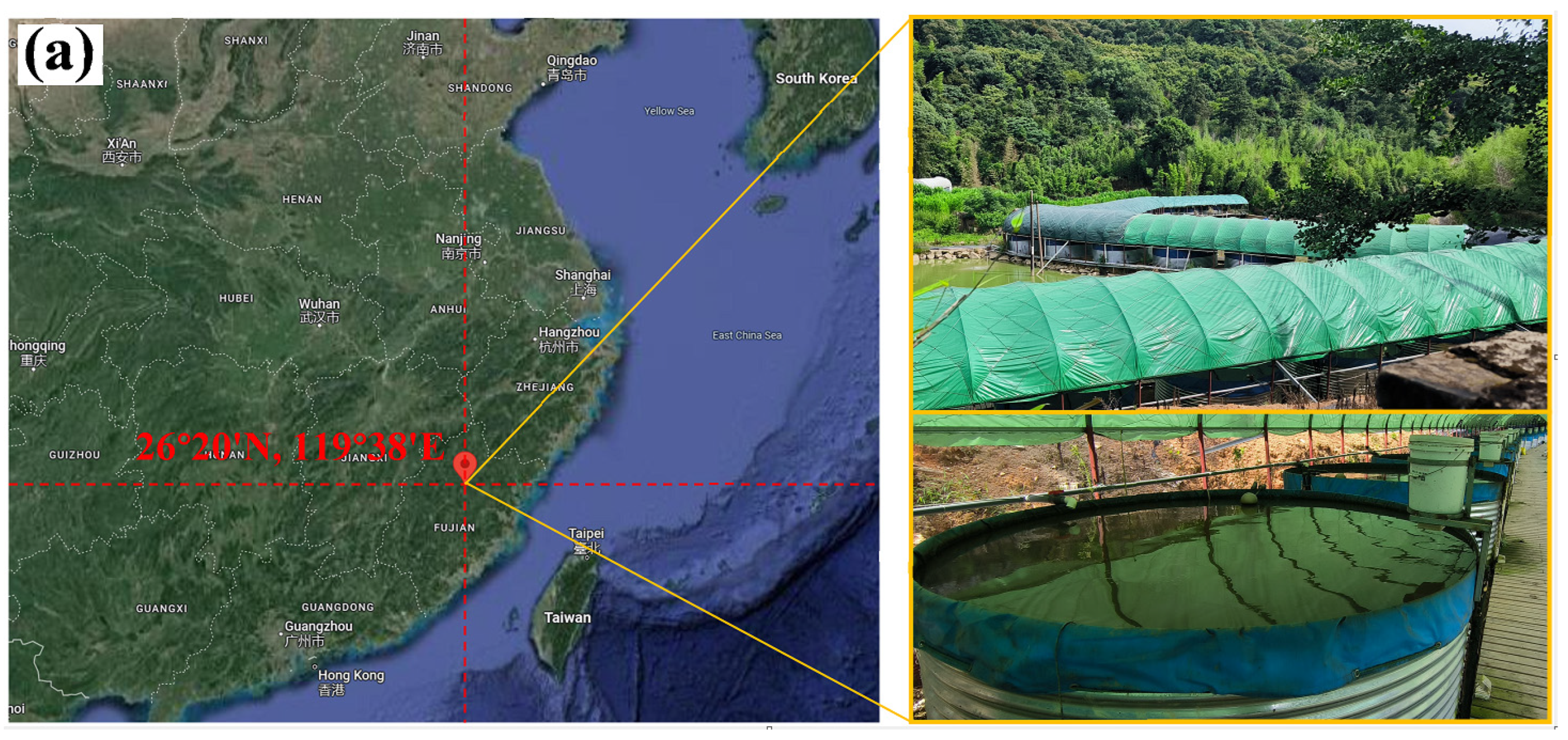
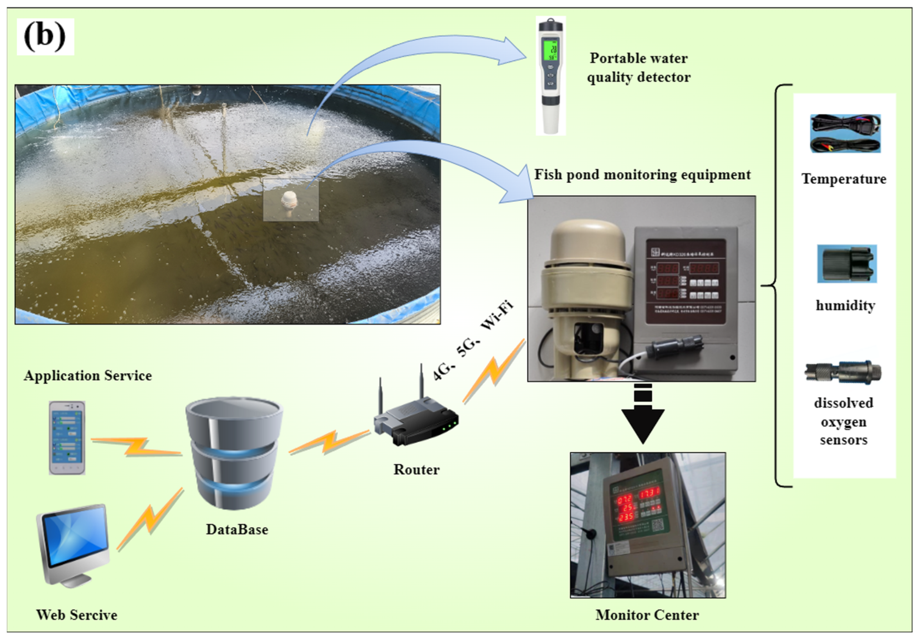
2.1. Experimental Data Collection

In this paper, the experimental data were collected from 7 to 14 August 2022 at the Mycorrhizal Microbial Agriculture Practice Base, Huanxi Town, Jin an District, Fuzhou City, Fujian Province, China (26°20′ N, 119°38′ E). The base is mainly used for the research of fungus culture technology and fungus bait microbial water high-density fish culture system, equipped with 37 high-density fish ponds, which can realize automatic feeding and water circulation. Data acquisition equipment for fish pond dissolved oxygen is oxygenation control equipment (Kodak brand KD326-A), as shown in Figure 1. The device can accurately capture a variety of water quality parameters of the aquaculture water body, to achieve for the perch one-stop intelligent monitoring, high-pressure oxygen demand, but also to saving the data to a database for easy recording, providing a cell phone and Web services to achieve remote monitoring of real-time adjustment function. It is also equipped with a portable water quality testing pen, which can accurately detect the PH, total dissolved solids, conductivity, and other values of pond water quality. During the actual sampling period at 9:00 and 14:00 each day, the KD326-A equipment was placed on the surface of the ponds to detect and record the temperature and dissolved oxygen of the 37 aquaculture ponds, and then the water bodies of the 37 ponds were collected and tested for the values of PH, total dissolved solids, and conductivity with the portable water quality testing pen. The data distribution is shown in

Table 1. Descriptive statistics for water quality samples.

Sample Point	PH	Water Temperature (°C)	Dissolved Oxygen (mg/L)	Conductivity (μS/cm)	Salinity	Total Dissolved Solids (mg/L)
01	5.64	27.1	5.8	440	0.22	220
02	5.39	27.1	5.9	440	0.22	218
03	5.36	27.1	5.7	438	0.22	218
04	5.64	27.0	5.8	430	0.22	220
……	……	……	……	……	……	……
371	5.2	27.2	5.9	353	0.18	176
Min	5.17	25.9	3.4	19.7	0.03	10
Max.	6.97	28.2	9.9	512	0.26	256
Mean	6.04	26.8	6.4	275.7	0.14	136.7
Std	0.41	0.53	1.44	0.057	0.05	58.5

, and the minimum, maximum, mean, and standard deviation of each group of data are also labeled.

2.2. Data Preprocessing

2.2.1. Data Standardization and Normalization

The experiment measured a total of six sets of water quality data, including pH, water temperature, dissolved oxygen, conductivity, salinity, and total dissolved solids. As the six water quality parameters are inconsistent in terms of unit and dimension, and the value distribution is wide (3.4~512), if the dimensionality is not unified problems such as poor effect of the subsequent training model and slow convergence speed will be caused. Normalization of the data set to mean 0, variance 1, and standardized data within the interval [0, 1] can solve the problem of feature skewness with larger dimensions of the model. Hence, the results predicted by the model are biased to features with larger dimensions, while the impact of features with smaller value changes on the predicted results is ignored. At the same time, the standardized data can effectively maintain the capture of useful information and reduce the impact of error values on the model.

Dimensionless processing of datasets is a data preprocessing method often used before model training, of which standardization and normalization of data are the most commonly used. When the data x is centered on mean μ and then scaled by the standard deviation σ, the data will conform to a normal distribution with mean 0 and variance 1 (i.e., the standard normal distribution), and this process is known as data standardization (Standardization, also known as Z-score normalization), with the following formula:

$$f(x)=\frac{x-\mu }{\sigma }$$

(1)

where µ is the mean and $\sigma$ is the standard deviation. When the data x is centered according to the minimum value, and then scaled according to the extreme deviation, it will converge to between [0, 1] and this process is called data normalization (Normalization, also known as Min-Max Scaling), and the formula is as follows:

$$f(x)=\frac{x-min\left(x\right)}{\mathit{max}\left(x\right)-min\left(x\right)}$$

(2)

where x is the current sample value to be tested, $min\left(x\right)$ is the minimum value among all samples, and $\mathit{max}\left(x\right)$ is the maximum value among all samples [31].

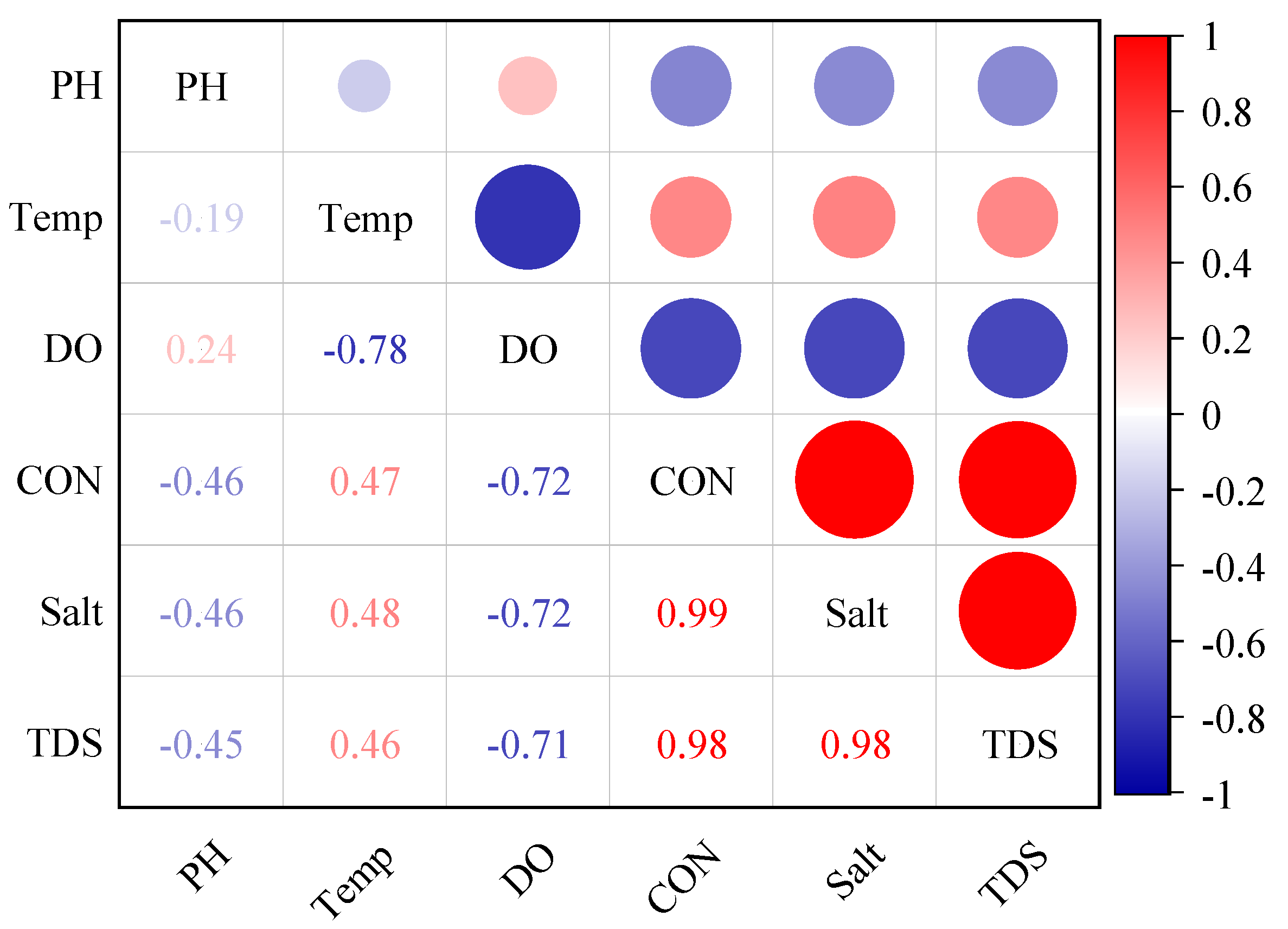
2.2.2. Data Correlation Analysis

Before model training, correlation analysis of the data features is the key to determining the speed of model training and convergence. In this paper, the DO was used as the dependent variable feature to be measured, and pH, water temperature, conductivity, salinity, and total dissolved solids were used as the independent variable features. In order to determine which independent variable features have a greater impact on the DO, PPMCC was used to determine the linear correlation between each feature and the DO. PPMCC is a measure of the strength of linear correlation between two variables x and y. It is usually used in regression analysis and numerical prediction with the following formula:

$$r_{x,y}=\frac{cov(X,Y)}{\sigma x\sigma y}$$

(3)

where $cov(X,Y)$ is the covariance of variables x and y, $\sigma x and \sigma y$ are the standard deviations of x and y, respectively. The value of r is between −1 and 1. The closer to −1, the more negatively correlated x and y are, the closer to 1, the more positively correlated x and y are, while near 0 indicates that x and y are not correlated. In general, if $\left|r\right|\ge 0.8$, the two variables can be considered highly correlated; if $0.5\le \left|r\right|<0.8$, the two variables can be considered moderately correlated; if $0.3\le \left|r\right|<0.5$, the two variables can be considered to be lowly correlated; if $\left|r\right|<0.3$, the two variables can be considered largely uncorrelated [32].

3. Data Modeling Methodology

3.1. Support Vector Regression (SVR)

SVR is an application of Support Vector Machines to regression problems, its main principle is to map low-dimensional linearly indivisible data into a high-dimensional linearly divisible space and find a hyperplane to divide it and realize the mapping with the help of the kernel function [33]. The ultimate goal of SVR is to find a regression function y such that the data are distributed as much as possible around y. The formula for f(x) is given below:

$$y=f\left(x\right)=\omega x+b$$

(4)

where x is the independent variable, $\omega$ is the set of vectors to be optimized, and b is the intercept. Meanwhile, when determining the decision boundary of SVR, the pursuit is to maximize the soft interval while minimizing the loss function. By maximizing the soft interval, it is realized to include as many data points as possible in the interval band of the support vectors, but in reality, it is difficult to artificially determine the support vector interval plane where it is located, so the slack variable ξ is introduced, which makes the interval requirement of the function become loose, after the introduction of the slack variable ξ, the loss function of SVR optimization can be expressed as:

$$\begin{array}{c}min\\ \omega ,b,{\xi }_i\end{array}\frac{{‖\omega ‖}^2}{2}+C \underset{i=1}{\sum ^n}{\xi }_i$$

(5)

$$subject to y_i\left(\omega ·\phi \left(x_i\right)+b\ge 1-{\xi }_i\right),$$

$${ \xi }_i\ge 0, i=1,\dots ,N$$

where ${\xi }_i$ is the slack variable, C is the penalty coefficient used to control the penalty term, and $\phi \left(x_i\right)$ is the set of points $x_i$ in low dimensions mapping to the high-dimensional space $\phi$ in the mapping function. Therefore, the loss function of the nonlinear SVR is obtained. From Equation (5), it can be seen that the loss function is a convex optimization problem in mathematics, and when solving such a convex optimization problem, the Lagrange multiplier method is usually used to solve it. First, the loss function is transformed into a Lagrangian function with constraints, and the solution of the original problem is equivalent to the solution of the dual function under the satisfaction of the Karlovski–Kuhn–Tucker (KKT) condition, so only the solution of the Lagrange dual function is required. Where the formula for the Lagrange dual function is as follows:

$$L_D=\underset{i=1}{\sum ^n}{\alpha }_i-\frac{1}{2}\underset{i,j=1}{\sum ^n}{\alpha }_i{\alpha }_j{y}_i{y}_i\phi \left(x_i\right)\phi \left(x_j\right)$$

(6)

$$subject to C\ge {\alpha }_i\ge 0$$

where ${\alpha }_i$ is the Lagrange operator, and $\phi \left(x_i\right)$ is the mapping function that maps the set of points $x_i$ to higher dimensions, but it is not clear exactly what mapping function is used to ensure that the decision boundary can be found in the transformed space, and when the computation of a dot product of the form $\phi \left(x_i\right)\phi \left(x_j\right)$, a kernel function needs to be introduced to solve the above problem. After the introduction of the kernel function, there is no need to know exactly what the mapping function is, and it is much easier to use the kernel function to compute the vector relations in low dimensions than in high dimensions $\phi \left(x_i\right)\phi \left(x_j\right)$. In this paper, according to the linear correlation analysis in the data preprocessing, it is found that there is a moderate degree of linear correlation between the DO content in water and other indicators, but at the same time, there is also a certain degree of nonlinear relationship. Therefore, the Gaussian radial basis partial linear kernel function (RBF) is chosen to transform the data from low latitude to high dimension with the following equation:

$$K\left(x,y\right)=e^{-\gamma {‖x-y‖}^2}, \gamma >0$$

(7)

where $\gamma$ is the parameter gamma to be optimized. As a result, the penalty coefficient C and the gamma parameter to be optimized in SVR can be obtained. In the following, the differential evolution and gray wolf optimization algorithm will be further combined to obtain the parameters to be optimized in SVR.

3.2. Differential Evolution (DE)

DE is an algorithm based on biological population differences and cross-evolution, which is proposed on the basis of genetic algorithms, and is commonly used to solve the overall optimal solution in a multi-dimensional space. With its powerful global search ability, DE has been widely used in the fields of constrained optimization, clustering optimization, nonlinear optimization, and neural network optimization, etc. The DE algorithm is to randomly initialize the population and take the fitness value of each individual in the population as the evaluation criterion, and the main process consists of three parts: variation, crossover, and selection. The basic idea of the algorithm is to apply the differences of individuals in the current population to reorganize to get the intermediate population, and then apply the offspring population to compete with the parent individuals to get the new generation population [34]. The advantage is that in the early stage of the algorithm, the individual differences of the populations are large, and the variation operation will make the algorithm have a strong global search ability, while in the late stage of the algorithm the individual differences of the populations are small, and the mutation operation will make the algorithm have a strong local search ability.

3.2.1. Population Initialization and Variation

After the DE algorithm performs a random initialization of the population $X_i\left(0\right)=\{x_{i,1}\left(0\right),x_{i,2}\left(0\right),x_{i,3}\left(0\right)\dots ,x_{i,n}\left(0\right) i=\mathrm{1,2},\dots ,n\}$, the DE algorithm will get the individuals of dimension n, where $x_{i,j}\left(0\right)$ is the value on dimension j of the i-individual in the population in generation 0, and then continue with the mutation operation. The DE algorithm will first select three individuals $X_{p1}\left(g\right)$, $X_{p2}\left(g\right)$, $X_{p3}\left(g\right)$ in the variation operation. After $X_{p2}\left(g\right)$ and $X_{p3}\left(g\right)$ get the differential value by scaling factor, it will add linearly with $X_{p1}\left(g\right)$, and the formula is as follows:

$$X_i\left(g\right)=X_{p1}\left(g\right)+F[X_{p2}\left(g\right)+X_{p3}\left(g\right)]$$

(8)

where $x_{p2}\left(g\right)+x_{p3}\left(g\right)$ is the differential vector; F is the scaling factor, which determines the step size of the individual differences of the population. The larger the F-value is, the global optimization ability of the algorithm will be enhanced, but the overall convergence speed of the algorithm will be affected.

3.2.2. Crossover of Populations

The crossover operation refers to the generation of a crossover population by utilizing some of the components of the individuals in the current population to be exchanged with the corresponding components in the mutated individuals according to some rule. The exchange rule here can be binomial crossover, i.e., for each component a random number within [0, 1] is generated, and if the number is less than the crossover operator then the exchange is performed, with the following formula:

$$U_{i,j}\left(g\right)=\left\{\begin{array}{c}{v}_{i,g}\left(g\right), if rand\left(j\right)<cr or j=r{n}_i\\ x_{i,j}\left(g\right), else \end{array}\right.$$

(9)

where $U_{i,j}\left(g\right)$ is the cross-population, and $rand\left(j\right)$ is a random number in [0, 1], the $r{n}_i$ is the random selection index, j is the number j component of an individual, and cr is the crossover operator.

3.2.3. Population Selection

In the DE algorithm, the current population will generate the intermediate population after completing the variation and crossover operations. The selection operation is to compare the fitness function values of the current population individuals with those of the intermediate population individuals, and to select the one with the best fitness value as the next-generation population individuals, which is formulated as follows:

$$X_i\left(g+1\right)=\left\{\begin{array}{c}{U}_i\left(g\right), f\left(V_i\left(g\right)\right)<f\left(X_i\right(g\left)\right)\\ X_i\left(g\right), else \end{array}\right.$$

(10)

where $f\left(V_i\left(g\right)\right)$ denotes the value of the fitness function of the mutant individual, if $U_i$ is better than $X_i$, it will be selected as the next generation. For each individual $X_i\left(g+1\right)$, it is always better than or equal to $X_i\left(g\right)$.

3.3. Gray Wolf Optimization (GWO)

GWO is a new type of pack intelligence optimization algorithm, which imitates the social hierarchy and hunting strategy of gray wolves in nature. It has been widely used in continuous optimization and combinatorial optimization problems in recent years. In the gray wolf optimization algorithm, the wolf pack is divided into four hierarchies, from high to low as $\alpha$ wolf, $\beta$ wolf, $\delta$ wolf and $\omega$ wolf. Among them, the gray wolves of higher ranks have absolute dominance over the gray wolves of lower ranks. There is one and only wolf in $\alpha$ wolf, $\beta$ wolf and $\delta$ wolf, and the $\omega$ hierarchy involves more than one. Where $\alpha$ wolf represents the optimal solution in the algorithm in each round, the $\beta$ wolf and $\delta$ wolf is the suboptimal solution. The $\omega$ wolves are subject to $\alpha$ wolf, $\beta$ wolf and $\delta$ wolf’s guidance to keep searching for new prey, and at the end of each round will re-update the $\alpha$ wolf’s position as the global optimal solution [35].

Suppose that the position of i wolf in an n-dimensional space is $X_i=(X_{i,1},X_{i,2},X_{i,3}\dots ,X_{i,n})$, the process of hunting can be divided into surrounding prey and hunting, where surrounding prey means that the i wolf updates its position information with prey under the guidance of $\alpha$ wolf, $\beta$ wolf and $\delta$ wolf. The formula is as follows:

$$\left\{\begin{array}{c}{X}_{\alpha ,i}=X_{\alpha }-A_1{D}_{\alpha }\\ X_{\beta ,i}=X_{\beta }-A_2{D}_{\beta }\\ X_{\delta ,i}=X_{\delta }-A_3{D}_{\delta }\end{array}\right.$$

(11)

where $X_{\alpha ,i}$, $X_{\beta ,i}$ and $X_{\delta ,i}$ are the position information of i wolf after being updated by $\alpha$ wolf, $\beta$ wolf and $\delta$ wolf, and A is the vector coefficients. D is formulated as follows:

$$\left\{\begin{array}{c}{D}_{\alpha }=\left|C_1{X}_{\alpha }-X_i\right|\\ D_{\beta }=\left|C_2{X}_{\beta }-X_i\right|\\ D_{\delta }=\left|C_3{X}_{\delta }-X_i\right|\end{array}\right.$$

(12)

where C is the relaxation factor. Thus, the process of i wolf surrounding the prey is obtained. The hunting process is described by the following formula:

$$X_i(t+1)=\frac{X_{\alpha ,i}+X_{\beta ,i}+X_{\delta ,i}}{3}$$

(13)

where $X_i(t+1)$ denotes the i wolf’s final position information, from Equation (13), GWO algorithm finds the global optimal solution through the guidance of $\alpha$, $\beta$ and $\delta$ wolves to $\omega$ wolves, not only can dynamically adjust the weight value, but also can effectively reduce the probability of falling into the local optimal.

3.4. Hybrid Differential Evolution and Gray Wolf Optimization Algorithm (DE-GWO-SVR)

In this paper, we propose to adopt the high-dimensional mapping based on the RBF kernel function. Therefore, the value of the mapping parameter gamma will play a decisive role in mapping the data from low to high dimensions, which affects the prediction speed and accuracy of the model. At the same time, the value of the penalty coefficient C in the SVR can directly determine the generalization ability of the model, the higher the C, the lower the tolerance of the model for error, and the model may fall into the overfitting state; the lower the C, the higher the tolerance of the model for error, and the model is can easily fall into the state of underfitting. Thus, the selection of C has a direct impact on the prediction accuracy of the model on the unknown DO value in this paper, and the GWO algorithm has the advantages of fast convergence and high accuracy of optimization algorithm parameters. So, this algorithm is used this paper to optimize C and gamma in SVR simultaneously. The fitness function formula is as follows:

$$Fitness=\frac{\sum _{i=1}^n{(y_i-\widehat{y_i})}^2}{n}\times 100$$

(14)

The GWO algorithm is a single algorithm that $\alpha$ wolf, $\beta$ wolf, $\delta$ wolf to guide other wolves in randomized hunts, if the $\alpha$ wolf, $\beta$ wolf and $\delta$ wolf fall into local optimum during random initialization, the whole algorithm will not be able to jump out of the local optimum solution to find the global optimum solution. Therefore, this paper proposes to fuse the DE algorithm with the GWO algorithm to maintain the population diversity by generating the next generation of wolves through differential evolution after each round of iteration, so as to improve the generalization ability of the model and jump out of the local optimal solution. Figure 2 shows the co-evolution process of the DE-GWO-SVR model and the steps to realize the prediction of DO content in perch aquaculture water using this algorithm.

Step 1 As shown in Figure 2, data preprocessing is first performed on the obtained water quality parameters to fill the missing values in the data and normalize the data so as to improve the convergence speed of the model in training. The dataset is divided into training, validation, and test sets. The training and validation sets are used to iterate the DE-GWO optimization algorithm.

Step 2 Initialize the parent, mutant and offspring wolves with the model parameters, the position of each wolf is assigned to the parameter C and gamma value in the SVR model, the fitness function value of the parent wolf needs to be computed once before the start of the iteration, the mean square error of the model for the validation set after each iteration is selected as the fitness function value, and the top three wolves with the optimal fitness function value are set to be $\alpha$ wolf, $\beta$ wolf, and $\delta$ wolf.

Step 3 Set the number of population iterations, during which it is first needed to keep on iterating according to the $\alpha$ wolf, $\beta$ wolf and $\delta$ wolf’s position to get the position of the other wolves that should be updated next. After traversing all the wolves, the top three wolves with optimal adaptation are selected as $\alpha$ wolf, $\beta$ wolf, and $\delta$ wolf next time. Then perform variation operation on each wolf in the current wolves, cross the mutated intermediate wolves with the parent wolves to generate the offspring wolves, and determine the offspring’s $\alpha$ wolf, $\beta$ wolf, and $\delta$ wolf before the next round of the cycle.

Step 4 When the population iteration is completed and the fitness function value tends to be stable and convergent, the position of $\alpha$ wolf in the current parent population is assigned to C and gamma in SVR, and SVR modeling is conducted on the test set through these parameters to predict the DO content in the perch aquaculture water body, and the model performance is evaluated and analyzed.

In this paper, we use the coefficient of determination (R²), Mean Square Error (MSE), Mean Absolute Error (MAE) and Root Mean Square Error (RMSE) for correlation analysis and model evaluation, which are calculated as follows:

$$R^2=1-\frac{\sum _{i=1}^n{(y_i-{\widehat{y}}_i)}^2}{\sum _{i=1}^n{(y_i-{\overline{y}}_i)}^2}$$

(15)

$$MSE=\frac{\sum _{i=1}^n{(y_i-\widehat{y_i})}^2}{n}$$

(16)

$$MAE=\frac{\sum _{i=1}^n\left|y_i-\widehat{y_i}\right|}{n}$$

(17)

$$RMSE=\sqrt{\frac{\sum _{i=1}^n{(y_i-\widehat{y_i})}^2}{n}}$$

(18)

where ${\widehat{y}}_i$ is the predicted value, $y_i$ is the observed value, ${\overline{y}}_i$ is the mean of the observations, and n is the total number of predicted samples. The prediction model of R² lies between [0, 1], the closer to 1 the better the model predicts, while the closer MSE, MAE, and RMSE are to, 0 the better the model is.

The models in this experiment are all run in a computer with Windows 11, CPU model R7-5800H, and graphics card model RTX3060. Coding in Matlab2022a with Python3.9 integrated in the environment of Anaconda3, and the machine learning framework is Scikit- based on the Python-3.9 learn framework.

4. Results and Discussion

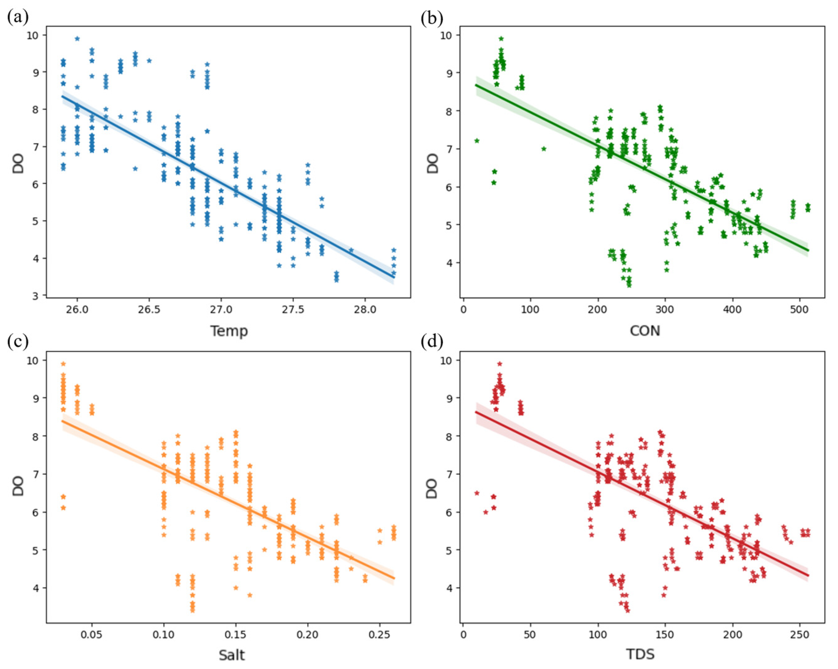
4.1. PPMCC Analysis of Water Quality Indicators

After standardization and normalization of the experimentally measured data of the six water qualities, the correlation analysis of PH, temperature, conductivity, salinity, total dissolved solids, and DO were performed, and the confusion matrix of the corresponding PPMCC values was obtained as shown in Figure 3. It can be seen from the results that the PPMCC values of DO and PH were only 0.244, and the PPMCC values with temperature, conductivity, salinity, and total organic salts were between −0.7 and −0.8. According to the range classification criteria of $\left|r\right|$, it can be assumed that there is little correlation between PH and DO, while the other characteristics are moderately correlated with DO. Therefore, according to the PPMCC value, the water quality data of temperature, conductivity, salinity and total dissolved solids that have a certain correlation with DO were initially screened.

Figure 4 further shows a two-dimensional scatter plot of the linear fit correlation between DO and Temp, CON, Salt, and TDS, respectively. The results depict that the proportion of dissolved oxygen can be explained by temperature is the highest, and there is an inverse ratio between the two, indicating that the higher the temperature in the pond, the lower the dissolved oxygen content in the water. Similarly, the electrical conductivity, salinity, and total organic salt content are inversely proportional to dissolved oxygen, indicating that the dissolved oxygen content in the water will decrease significantly when the water temperature, water salinity, and solid dissolved matter content are higher, which is not suitable for perch growth. It can also be concluded that the relationship between the dissolved oxygen and other parameters in water is partially linear based on Figure 3 and Figure 4.

4.2. Model Parameter Initialization and Validation of Fitness Function Values

After the data correlation analysis is performed to determine the characteristic data, the initialization parameter values of the DE-GWO-SVR model need to be determined. Five initialization hyperparameters were set in the experiments of this paper, in which the initialization population size (nPop) was 30, the maximum number of iterations (MaxIt) was 500, the independent variable dimension (nVar) was 2, the crossover probability (pCR) was 0.2, and the scaling factor (Beta) was between 0.2 and 0.8. This setting not only satisfies the number of wolves in each generation in the GWO algorithm, but also satisfies the variation operation of the population in the DE algorithm, as well as balancing the time for optimization of the algorithm. In performing the experimental simulation, according to Equations (14) and (15), 100 times MSE value with R² value as the objective function value was selected for optimization, which can make sure that the optimization avoids the disappearance of error due to the lack of precision. Figure 5 shows the fitness function graph of the algorithm during 500 iterations of the experimental simulation. As shown, with the continuous iteration of the optimization algorithm, the mean square error value of the algorithm is decreasing and the fitness of the algorithm is increasing. After the first 400 rounds of optimization, the curve fluctuation amplitude is significantly reduced and tends to be stable, which indicate that the fitness of the algorithm at this time has reached an optimal state, and the fitness function value no longer continues to decline with the iteration of the algorithm.

4.3. Comparative Analysis of Residual Values for Water Quality DO Predictions

With the optimal parameters of the DE-GWO-SVR model set, the model training was carried out according to the process shown in Figure 2. First, through the PPMCC analysis, the feature of PH was excluded, the rest of the features were retained, the division of the training set and test set was done, and then the initialization parameters of the model were set up as shown in Figure 5, and the prediction of DO in the aquaculture water body of the California perch fish was carried out. In order to compare and validate the performance of the DE-GWO-SVR model, the BPNN and its optimized models (GA-BPNN, PSO-BPNN, GWO-BPNN, DE-GWO-BPNN), and the SVR and its optimized models (GA-SVR, PSO-SVR, GWO-SVR) were also selected to predict the DO content, and the results are shown in Figure 6. Here in this paper, each test model was tuned with initial parameters and set the number of training times 500 times against the DE-GWO-SVR model. By comparing the degree of difference between the model-fitted prediction curves and the original data curves, it can be seen that the prediction effect based on SVR and its optimization model is generally better than that based on BPNN and its optimization model.

As can be seen in Figure 6, the SVR model using hybrid DE-GWO optimization is more accurate in predicting the DO compared to the other models, and fits the real data better. The RBF kernel was chosen as the kernel function of the SVR model, which improved the nonlinear fitting ability of the model. In addition, the DE optimization algorithm was introduced to cross-mutate the GWO algorithm for the population, so that the GWO optimization algorithm further improved the global search ability with its own excellence. Therefore, it can accurately predict the values of the nonlinearly correlated. Subsequently, the performance of the DE-GWO-SVR optimization model used in this paper was further verified by calculating the residual values by each model for the prediction of DO in the California perch water. As shown in Figure 6, the residual values obtained from the prediction of dissolved oxygen in California perch water using the DE-GWO-SVR model had an upper quartile of 0.2185 and a lower quartile of −0.2363, with a small fluctuation range of the residual values. Compared with the SVR model without the optimization algorithm, the upper quartile of the residual values of the DE-GWO-SVR model is lower by 0.1601 and the lower quartile is higher by 0.1535. Compared with the SVR model optimized with the PSO, the upper quartile and the lower quartile of the SVR model are lower by 0.1256 and higher by 0.1859, respectively. Compared with the SVR model optimized using the GWO, the two have the closest and smaller residual ranges (the residual values are distributed near the baseline location). In addition, it can be seen from Figure 6 that the residual value of the results predicted by the BPNN model fluctuates the most. The upper quartile of 0.495 is much higher than the result of the DE-GWO-SVR hybrid optimization prediction model, and the lower quartile of −0.3892 is also much lower than the result of DE-GWO-SVR. The predictive performance of the BPNN and its optimized model is lower than that of the non-optimized SVR model. Although the residual value of the GA-BPNN model is small in general, the deviation of individual predicted value is too large. Through the above analysis, it can be seen that the DE-GWO hybrid optimization strategy used in this paper can effectively improve the prediction accuracy of the model, and the optimized model has good stability for the prediction of dissolved oxygen in the water of California perch.

4.4. Comparative Analysis of Different Optimization Models on DO Prediction Performance

In this paper, the optimization results of the SVR model and the BPNN model are compared between the conventional optimization algorithms (GA, PSO, GWO) and the proposed hybrid optimization algorithm (DE-GWO). As shown in Figure 7, the horizontal coordinate of each subgraph is the true value, and the vertical coordinate is the predicted value. The dotted line in the figure is the regression line when the predicted value is equal to the true value. Herein, the more scattered points in the figure are concentrated on both sides of the regression line, the closer the predicted value of the model is to the true value. Compared with other models, the scatter-value distribution of the proposed DE-GWO-SVR hybrid optimization model is more concentrated on both sides of the regression line, indicating that its prediction accuracy is higher.

Table 2. Comparison of error assessment of DE-GWO hybrid optimization with other optimization algorithms.

Model\Indicators	R2	MSE	MAE	RMSE
BPNN	0.73	0.484	0.5434	0.6961
GA-BPNN	0.81	0.334	0.3971	0.5785
PSO-BPNN	0.86	0.254	0.3889	0.5043
GWO-BPNN DE-GWO-BPNN	0.84 0.86	0.294 0.245	0.4051 0.3391	0.5427 0.4952
SVR	0.78	0.396	0.4792	0.6294
GA-SVR	0.89	0.202	0.2696	0.4502
PSO-SVR	0.86	0.253	0.4221	0.5040
GWO-SVR	0.91	0.163	0.3076	0.4038
DE-GWO-SVR	0.94	0.108	0.2629	0.3293

further lists the DE-GWO-SVR and DE-GWO-BPNN hybrid optimization models and the SVR, GA-SVR, PSO-SVR, GWO-SVR, BPNN, GA-BPNN, PSO-BPNN, and GWO-BPNN models with the corresponding R², MSE, MAE, and RMSE evaluation index. From the results, it can be seen that the SVR base model predicts DO better than the BPNN. Due to the fact that the parameter transfer between individual neurons of the BPNN model is linear, and only the activation function can be selected as a nonlinear activation function (e.g., sigmoid and ReLU activation function). The BPNN cannot have good prediction of the nonlinear metrics when the model is trained, whereas the SVR model that has used RBF kernel functions can fit a hyperplane to uplift and re-divide the data when the model is trained, attributes to the advantage of SVR in nonlinear prediction. The performance of the SVR model optimized by the GA, PSO, and GWO is overall better than the corresponding BPNN optimized model, in which the prediction accuracy of the PSO-BPNN and the PSO-SVR model is comparable. The main reason is that when the PSO optimization algorithm is searching for the optimal parameters, there is no priority among the particle swarms. The network structure of the BPNN model can be changed arbitrarily within a certain range, which has a certain probability of jumping out of the local optimum, but it is still not as good as the optimization effect of the GWO-SVR model. In this respect, the SVR was selected as the base model for algorithm optimization. By comparing the performance of the optimization algorithms, it can be seen that the optimization performance of the GA, GWO, and PSO on the prediction results of the BPNN model is improved successively (R² values of 0.81, 0.84 and 0.86, respectively), and its optimization effect is improved by 9.88%, 13.09%, and 15.12%, respectively, compared with that of the un-optimized BPNN base model (R² = 0.73). The optimization performance of the PSO, GA, and GWO on the SVR model is improved successively (R² values of 0.86, 0.89, and 0.91, respectively), which improved their optimization performance by 9.30%, 12.36%, and 14.28%, respectively, compared to the un-optimized SVR base model (R² = 0.78). The results show that the PSO has the best optimization effect on the BPNN and the worst optimization effect on the SVR, indicating that the PSO has a large variability in optimizing different base models and its optimization performance is unstable. Comparing the GA and GWO algorithms, the optimization accuracy and stability of the GWO for the two groups of basis models are better than that of the GA, indicating that the GWO has better model optimization performance. Therefore, in this paper we choose the SVR as the base model and the GWO as the optimization algorithm, and further adopt the DE algorithm for model optimization that propose the DE-GWO-SVR hybrid optimization model. Its prediction correlation coefficient achieves the highest value of R² = 0.94, and the error indicators MSE, MAE, and RMSE all achieve the corresponding lowest values of MSE = 0.108, MAE = 0.2629, and RMSE = 0.3293, respectively, which improves the prediction accuracy by 17.02% compared with that of the SVR base model.

5. Conclusions

In this paper a DE-GWO-SVR model based on second-order hybrid optimization is proposed for accurate and reliable prediction of DO in California perch aquaculture water bodies. Based on the data preprocessing and prediction model optimized with the objective, adopts PPMCC correlation analysis and regression analysis, realizes the dimensionality reduction of the water quality multi-parameter data, and improves the quality of the data. The structure of with hybrid optimization of the DE-GWO and combined weight coefficient optimization with parameter initialization and validation of fitness function value solves the dilemma of traditional single optimization algorithm, which can easily fall into local optimum. The DE-GWO-SVR model constructed in this paper can effectively characterize water quality factors with multivariate, coupling, and nonlinear characteristics, but also can avoid the limitations of traditional methods in terms of small samples, high dimensionality and overfitting. Compared with the SVR, BPNN, and their optimization models, the method in this paper not only improves the accuracy of model prediction, but also the training set of the fitness function has a good convergence effect, and it has achieved a more reliable application effect in water quality DO content prediction, which provides a new idea for high-precision and high-efficiency prediction of water quality factors in complex aquaculture water bodies.

References

1. Zhang, X.; Zhang, Y.; Zhang, Q.; Liu, P.; Guo, R.; Jin, S.; Liu, Y. Evaluation and analysis of water quality of marine aquaculture area. Int. J. Environ. Res. Public Health 2020, 17, 1446. [Google Scholar] [CrossRef] [PubMed]
2. Wei, Y.; Wei, Q.; An, D. Intelligent monitoring and control technologies of open sea cage culture: A review. Comput. Electron. Agric. 2020, 169, 105119. [Google Scholar] [CrossRef]
3. Mai, C. Transforming the Growth Mode is the Only Way for the Sustainable Development of Aquaculture in China. Fish. Inf. Strategy 2012, 27, 1–6. [Google Scholar]
4. Jiang, X.; Dong, S.; Liu, R.; Huang, M.; Dong, K.; Ge, J.; Zhou, Y. Effects of temperature, dissolved oxygen, and their interaction on the growth performance and condition of rainbow trout (Oncorhynchus mykiss). J. Therm. Biol. 2021, 98, 102928. [Google Scholar] [CrossRef] [PubMed]
5. Reddythota, D.; Timotewos, M.T. Evaluation of Pollution Status and Detection of the Reason for the Death of Fish in Chamo Lake, Ethiopia. J. Environ. Public Health 2022, 2022, 5859132. [Google Scholar] [CrossRef] [PubMed]
6. Loos, S.; Shin, C.M.; Sumihar, J.; Kim, K.; Cho, J.; Weerts, A.H. Ensemble data assimilation methods for improving river water quality forecasting accuracy. Water Res. 2020, 171, 115343. [Google Scholar] [CrossRef] [PubMed]
7. Asadollah, S.B.H.S.; Sharafati, A.; Motta, D.; Motta, D.; Yaseen, Z.M. River water quality index prediction and uncertainty analysis: A comparative study of machine learning models. J. Environ. Chem. Eng. 2021, 9, 104599. [Google Scholar] [CrossRef]
8. Su, X.; He, X.; Zhang, G.; Chen, Y.; Li, K. Research on SVR water quality prediction model based on improved sparrow search algorithm. Comput. Intell. Neurosci. 2022, 2022, 7327072. [Google Scholar] [CrossRef] [PubMed]
9. Jamroen, C.; Yonsiri, N.; Odthon, T.; Wisitthiwong, N.; Janreung, S. A standalone photovoltaic/battery energy-powered water quality monitoring system based on narrowband internet of things for aquaculture: Design and implementation. Smart Agric. Technol. 2023, 3, 100072. [Google Scholar] [CrossRef]
10. Mashala, M.J.; Dube, T.; Mudereri, B.T.; Ayisi, K.K.; Ramudzuli, M.R. A Systematic Review on Advancements in Remote Sensing for Assessing and Mon-itoring Land Use and Land Cover Changes Impacts on Surface Water Resources in Semi-Arid Tropical Environments. Remote Sens. 2023, 15, 3926. [Google Scholar] [CrossRef]
11. Prapti, D.R.; Mohamed Shariff, A.R.; Che Man, H.; Ramli, N.M.; Perumal, T.; Shariff, M. Internet of Things (IoT)-based aquaculture: An overview of IoT application on water quality monitoring. Rev. Aquac. 2022, 14, 979–992. [Google Scholar] [CrossRef]
12. Rastegari, H.; Nadi, F.; Lam, S.S.; Abdullah, M.I.; Kasan, N.A.; Rahmat, R.F.; Mahari, W.A.W. Internet of Things in aquaculture: A review of the challenges and potential solutions based on current and future trends. Smart Agric. Technol. 2023, 4, 100187. [Google Scholar] [CrossRef]
13. Ustaoğlu, F.; Tepe, Y.; Taş, B. Assessment of stream quality and health risk in a subtropical Turkey river system: A combined approach using statistical analysis and water quality index. Ecol. Indic. 2020, 113, 105815. [Google Scholar] [CrossRef]
14. Zhi, W.; Feng, D.; Tsai, W.P.; Sterle, G.; Harpold, A.; Shen, C.; Li, L. From hydrometeorology to river water quality: Can a deep learning model predict dissolved oxygen at the continental scale? Environ. Sci. Technol. 2021, 55, 2357–2368. [Google Scholar] [CrossRef]
15. Huan, J.; Li, H.; Li, M.; Chen, B. Prediction of dissolved oxygen in aquaculture based on gradient boosting decision tree and long short-term memory network: A study of Chang Zhou fishery demonstration base, China. Comput. Electron. Agric. 2020, 175, 105530. [Google Scholar] [CrossRef]
16. Li, W.; Wu, H.; Zhu, N.; Jiang, Y.; Tan, J.; Guo, Y. Prediction of dissolved oxygen in a fishery pond based on gated recurrent unit (GRU). Inf. Process. Agric. 2021, 8, 185–193. [Google Scholar] [CrossRef]
17. Tung, T.M.; Yaseen, Z.M. A survey on river water quality modelling using artificial intelligence models: 2000–2020. J. Hydrol. 2020, 585, 124670. [Google Scholar]
18. Jiang, Y.; Nan, Z.; Yang, S. Risk assessment of water quality using Monte Carlo simulation and artificial neural network method. J. Environ. Manag. 2013, 122, 130–136. [Google Scholar] [CrossRef]
19. Kadam, A.K.; Wagh, V.M.; Muley, A.A.; Umrikar, B.N.; Sankhua, R.N. Prediction of water quality index using artificial neural network and multiple linear regression modelling approach in Shivganga River basin, India. Model. Earth Syst. Environ. 2019, 5, 951–962. [Google Scholar] [CrossRef]
20. Zare Abyaneh, H. Evaluation of multivariate linear regression and artificial neural networks in prediction of water quality parameters. J. Environ. Health Sci. Eng. 2014, 12, 40. [Google Scholar] [CrossRef]
21. Khan MS, I.; Islam, N.; Uddin, J.; Islam, S.; Nasir, M.K. Water quality prediction and classification based on principal component regression and gradient boosting classifier approach. J. King Saud Univ. Comput. Inf. Sci. 2022, 34, 4773–4781. [Google Scholar]
22. Xu, C.; Chen, X.; Zhang, L. Predicting river dissolved oxygen time series based on stand-alone models and hybrid wavelet-based models. J. Environ. Manag. 2021, 295, 113085. [Google Scholar] [CrossRef]
23. Li, Z.; Peng, F.; Niu, B.; Wu, J.; Miao, Z. Water quality prediction model combining sparse auto-encoder and LSTM network. IFAC Pap. 2018, 51, 831–836. [Google Scholar] [CrossRef]
24. Paine, A.; Wokingham, U.K. Distribution, and Reproduction in any Medium, Provided the Original Work Is Properly Cited; Wiley: Hoboken, NJ, USA, 2020. [Google Scholar]
25. Guo, J.; Dong, J.; Zhou, B.; Zhao, X.; Liu, S.; Han, Q.; Hassan, S.G. A hybrid model for the prediction of dissolved oxygen in seabass farming. Comput. Electron. Agric. 2022, 198, 106971. [Google Scholar] [CrossRef]
26. Huang, J.; Liu, S.; Hassan, S.G.; Xu, L.; Huang, C. A hybrid model for short-term dissolved oxygen content prediction. Comput. Electron. Agric. 2021, 186, 106216. [Google Scholar] [CrossRef]
27. Zhang, J.; Zhang, Y.; Chen, L.; Wang, Q.; Zhao, M. Water Quality Prediction for Hanjiang with Optimized Support Vector Regression. In Proceedings of the 2019 IEEE 8th Data Driven Control and Learning Systems Conference (DDCLS), Dali, China, 24–27 May 2019; IEEE: Piscataway, NJ, USA, 2019; pp. 832–837. [Google Scholar]
28. Li, T.; Lu, J.; Wu, J.; Zhang, Z.; Chen, L. Predicting Aquaculture Water Quality Using Machine Learning Approaches. Water 2022, 14, 2836. [Google Scholar] [CrossRef]
29. Negi, G.; Kumar, A.; Pant, S.; Pant, S.; Ram, M. GWO: A review and applications. Int. J. Syst. Assur. Eng. Manag. 2021, 12, 1–8. [Google Scholar] [CrossRef]
30. Deng, W.; Shang, S.; Cai, X.; Zhao, H.; Song, Y.; Xu, J. An improved differential evolution algorithm and its application in optimization problem. Soft Comput. 2021, 25, 5277–5298. [Google Scholar] [CrossRef]
31. Singh, D.; Singh, B. Investigating the impact of data normalization on classification performance. Appl. Soft Comput. 2020, 97, 105524. [Google Scholar] [CrossRef]
32. Shrestha, N. Factor analysis as a tool for survey analysis. Am. J. Appl. Math. Stat. 2021, 9, 4–11. [Google Scholar] [CrossRef]
33. Zhang, F.; O’Donnell, L.J. Support Vector Regression. In Machine Learning; Academic Press: New York, NY, USA, 2020; pp. 123–140. [Google Scholar]
34. Opara, K.R.; Arabas, J. Differential Evolution: A survey of theoretical analyses. Swarm Evol. Comput. 2019, 44, 546–558. [Google Scholar] [CrossRef]
35. Sharma, I.; Kumar, V.; Sharma, S. A comprehensive survey on grey wolf optimization. Recent Adv. Comput. Sci. Commun. 2022, 15, 323–333. [Google Scholar]
Figure 1. Experimental base and water quality data collection diagram. (a) Location map of the testing site, (b) Experimental data collection flowchart.
Applsci 14 00856 g001aApplsci 14 00856 g001b
Figure 2. Flowchart of optimization of DE-GWO-SVR model.
Applsci 14 00856 g002
Figure 3. PPMCC−based water quality data analysis diagram.
Applsci 14 00856 g003
Figure 4. Univariate linear fit between temperature, conductivity, salinity, total dissolved solids, and dissolved oxygen. (a) DO and temperature, (b) DO and conductivity, (c) DO and salinity, (d) DO and total dissolved solids.
Applsci 14 00856 g004
Figure 5. Plot of fitness function for hybrid DE-GWO optimization.
Applsci 14 00856 g005
Figure 6. Prediction results and residual graphs of various optimization algorithms when BPNN and SVR are used as base models to be optimized for DO forecast. (a) BPNN, (b) SVR, (c) GA−BPNN, (d) GA−SVR, (e) PSO−BPNN, (f) PSO−SVR, (g) GWO−BPNN, (h) GWO−SVR, (i) DE−GWO−BPNN, (j) DE−GWO−SVR.
Applsci 14 00856 g006aApplsci 14 00856 g006b
Figure 7. Comparison of prediction results between DE-GWO-SVR hybrid optimization algorithm and other different optimization algorithms. (a) BPNN, (b) SVR, (c) GA-BPNN, (d) GA-SVR, (e) PSO-BPNN, (f) PSO-SVR, (g) GWO-BPNN, (h) GWO-SVR, (i) DE-GWO-BPNN.
Applsci 14 00856 g007