
An Integrated Lean and Six Sigma Framework for Improving Productivity Performance: A Case Study in a Spanish Chemicals Manufacturer


Abstract
:1. Introduction
Literature Review
2. Materials and Methods
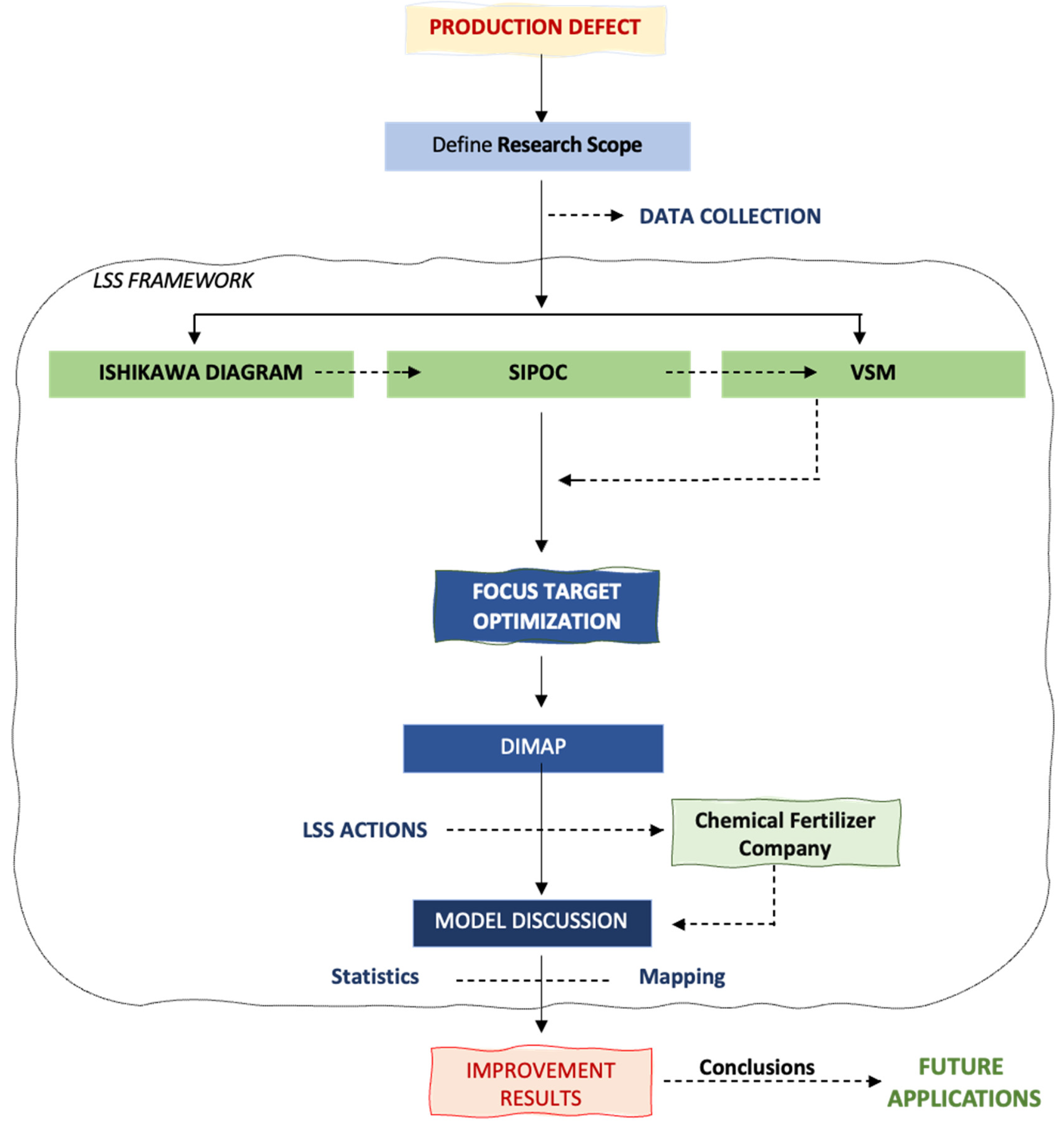
2.1. Lean Tools Deployment
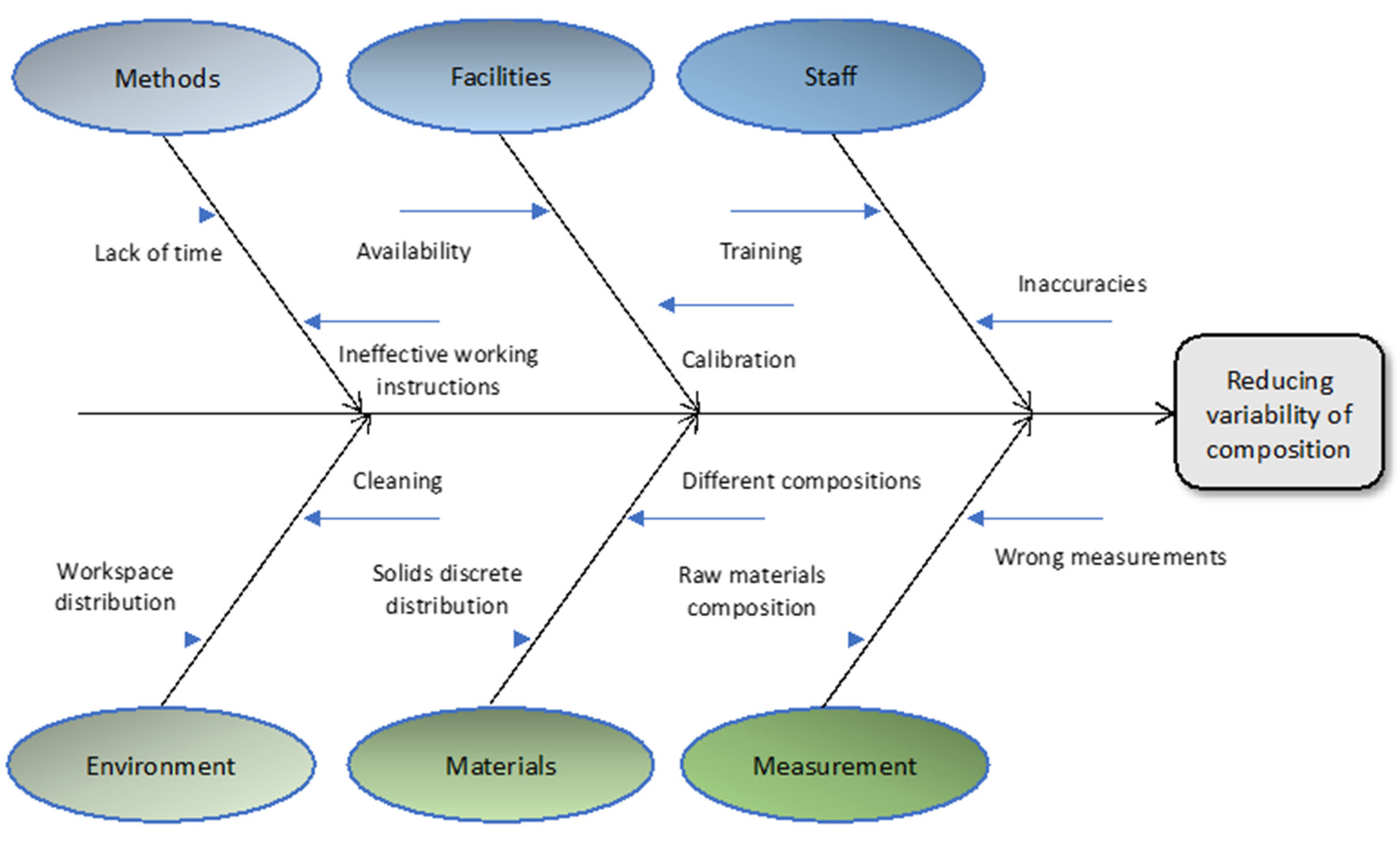
2.1.1. Ishikawa Diagram
2.1.2. SIPOC Diagram
2.1.3. Value Stream Map
3. Results and Discussion
3.1. Define
3.2. Measure

| Test | D2R kg/L | Y21R kg C21R/kg T | Y22R kg C22R/kg T | Y21T − Y21R kg C21/kg T | Y22T − Y22R kg C22/kg T | D2T − D2R kg/L |
|---|---|---|---|---|---|---|
| 1 | 1.328 | 0.610 | 0.031 | −0.010 | −0.001 | 0.002 |
| 2 | 1.328 | 0.610 | 0.031 | −0.010 | −0.001 | 0.002 |
| 3 | 1.332 | 0.603 | 0.032 | −0.003 | −0.002 | −0.002 |
| 4 | 1.309 | 0.596 | 0.031 | 0.004 | −0.001 | 0.021 |
| 5 | 1.328 | 0.610 | 0.033 | −0.010 | −0.003 | 0.002 |
| 6 | 1.324 | 0.599 | 0.030 | 0.001 | 0.000 | 0.006 |
| 7 | 1.325 | 0.600 | 0.030 | 0.000 | 0.000 | 0.005 |
| 8 | 1.325 | 0.600 | 0.030 | 0.000 | 0.000 | 0.005 |
| 9 | 1.328 | 0.600 | 0.030 | 0.000 | 0.000 | 0.002 |
| 10 | 1.328 | 0.598 | 0.028 | 0.002 | 0.002 | 0.002 |
| 11 | 1.328 | 0.600 | 0.030 | 0.000 | 0.000 | 0.002 |
| 12 | 1.330 | 0.598 | 0.030 | 0.002 | 0.000 | 0.000 |
| 13 | 1.331 | 0.591 | 0.030 | 0.009 | 0.000 | −0.001 |
| 14 | 1.333 | 0.602 | 0.031 | −0.002 | −0.001 | −0.003 |
| 15 | 1.331 | 0.582 | 0.030 | 0.018 | 0.000 | −0.001 |
| 16 | 1.332 | 0.592 | 0.032 | 0.008 | −0.002 | −0.002 |
| 17 | 1.335 | 0.598 | 0.031 | 0.002 | −0.001 | −0.005 |
| 18 | 1.330 | 0.593 | 0.028 | 0.007 | 0.002 | 0.000 |
| 19 | 1.327 | 0.600 | 0.030 | 0.000 | 0.000 | 0.003 |
| 20 | 1.336 | 0.600 | 0.029 | 0.000 | 0.001 | −0.006 |
| 21 | 1.320 | 0.595 | 0.025 | 0.005 | 0.005 | 0.010 |
| 22 | 1.320 | 0.595 | 0.025 | 0.005 | 0.005 | 0.010 |
| 23 | 1.328 | 0.598 | 0.029 | 0.002 | 0.001 | 0.002 |
| 24 | 1.327 | 0.600 | 0.028 | 0.000 | 0.002 | 0.003 |
| 25 | 1.328 | 0.598 | 0.028 | 0.002 | 0.002 | 0.002 |
| 26 | 1.328 | 0.598 | 0.028 | 0.002 | 0.002 | 0.002 |
| 27 | 1.327 | 0.598 | 0.030 | 0.002 | 0.000 | 0.003 |
| 28 | 1.328 | 0.600 | 0.035 | 0.000 | −0.005 | 0.002 |
| 29 | 1.330 | 0.600 | 0.030 | 0.000 | 0.000 | 0.000 |
| 30 | 1.332 | 0.595 | 0.030 | 0.005 | 0.000 | −0.002 |
| 31 | 1.300 | 0.590 | 0.027 | 0.010 | 0.003 | 0.030 |
| 32 | 1.332 | 0.597 | 0.028 | 0.003 | 0.002 | −0.002 |
| 33 | 1.332 | 0.596 | 0.028 | 0.004 | 0.002 | −0.002 |
| 34 | 1.330 | 0.600 | 0.030 | 0.000 | 0.000 | 0.000 |
| 35 | 1.331 | 0.600 | 0.030 | 0.000 | 0.000 | −0.001 |
| Test | D3R kg/L | Y31R kg C31R/kg T | Y31T − Y31R kg C31/kg T | D3T − D3R kg/L |
|---|---|---|---|---|
| 1 | 1.162 | 0.052 | −0.011 | −0.012 |
| 2 | 1.162 | 0.052 | −0.011 | −0.012 |
| 3 | 1.163 | 0.051 | −0.010 | −0.013 |
| 4 | 1.163 | 0.047 | −0.006 | −0.013 |
| 5 | 1.145 | 0.047 | −0.006 | 0.005 |
| 6 | 1.145 | 0.045 | −0.004 | 0.005 |
| 7 | 1.159 | 0.047 | −0.006 | −0.009 |
| 8 | 1.160 | 0.045 | −0.004 | −0.010 |
| 9 | 1.160 | 0.047 | −0.006 | −0.010 |
| 10 | 1.160 | 0.042 | −0.001 | −0.010 |
| 11 | 1.160 | 0.042 | −0.001 | −0.010 |
| 12 | 1.145 | 0.039 | 0.002 | 0.005 |
| 13 | 1.145 | 0.038 | 0.003 | 0.005 |
| 14 | 1.162 | 0.041 | 0.000 | −0.012 |
| 15 | 1.142 | 0.044 | −0.003 | 0.008 |
| 16 | 1.142 | 0.044 | −0.003 | 0.008 |
| 17 | 1.144 | 0.045 | −0.004 | 0.006 |
| 18 | 1.144 | 0.045 | −0.004 | 0.006 |
| 19 | 1.149 | 0.047 | −0.006 | 0.001 |
| 20 | 1.163 | 0.041 | 0.000 | −0.013 |
| 21 | 1.161 | 0.047 | −0.006 | −0.011 |
| 22 | 1.161 | 0.049 | −0.008 | −0.011 |
| 23 | 1.160 | 0.045 | −0.004 | −0.010 |
| 24 | 1.145 | 0.045 | −0.004 | 0.005 |
| 25 | 1.145 | 0.045 | −0.004 | 0.005 |
| 26 | 1.153 | 0.047 | −0.006 | −0.003 |
| 27 | 1.160 | 0.048 | −0.007 | −0.010 |
| 28 | 1.160 | 0.048 | −0.007 | −0.010 |
| 29 | 1.172 | 0.048 | −0.007 | −0.022 |
| 30 | 1.173 | 0.050 | −0.009 | −0.023 |
| 31 | 1.173 | 0.052 | −0.011 | −0.023 |
| 32 | 1.179 | 0.049 | −0.008 | −0.029 |
| 33 | 1.157 | 0.046 | −0.005 | −0.007 |
| 34 | 1.172 | 0.040 | 0.001 | −0.022 |
| 35 | 1.153 | 0.037 | 0.004 | −0.003 |
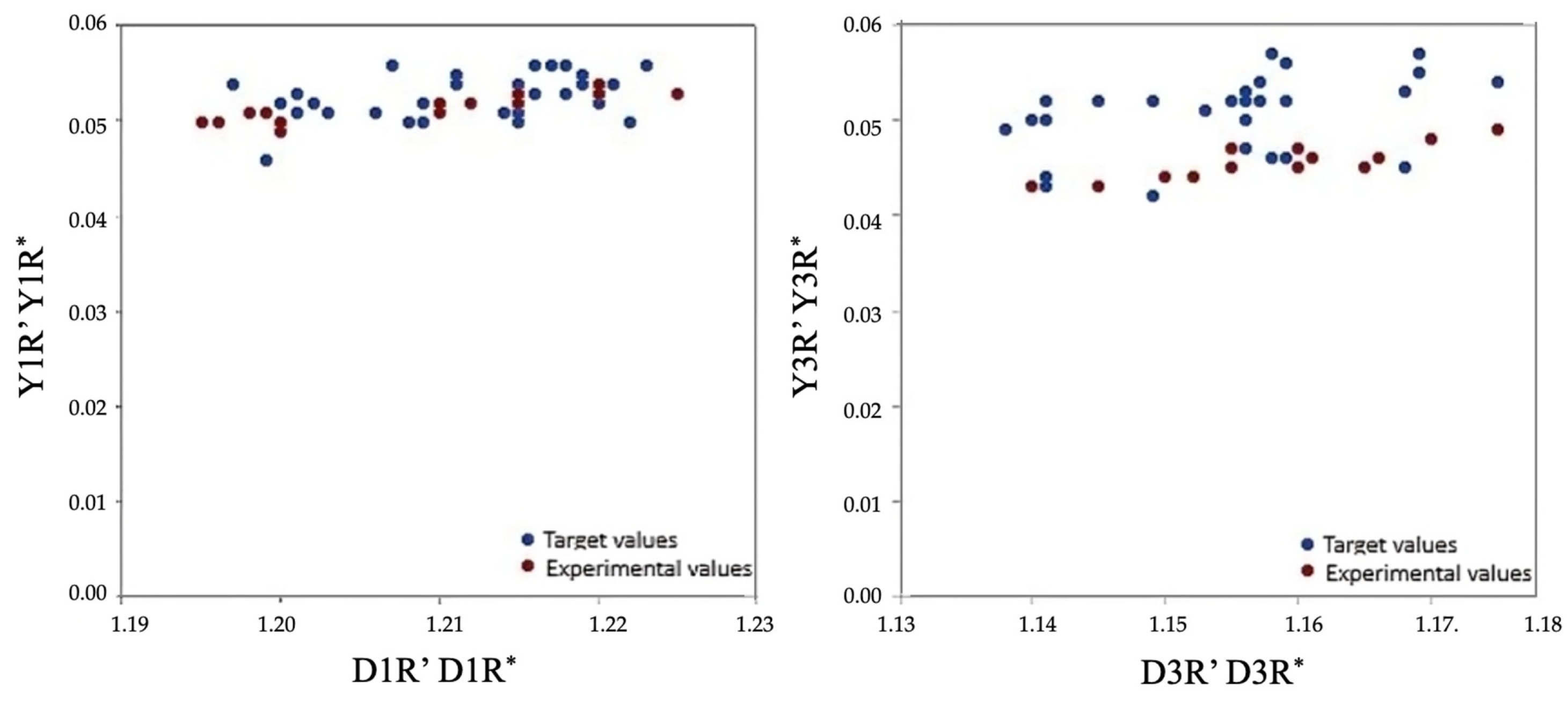
3.3. Analyze
3.4. Improve
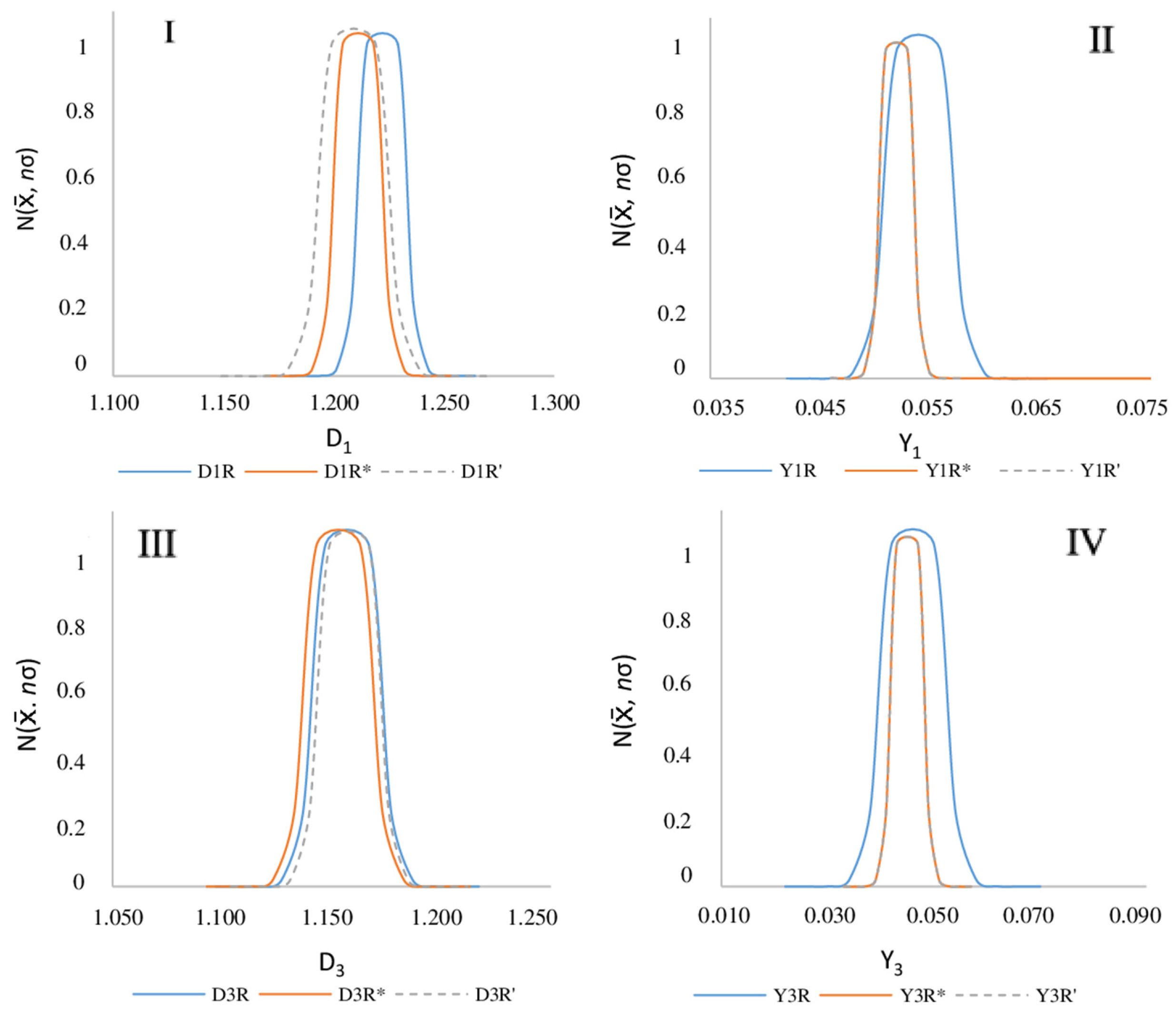
3.5. Control
| Test | D3R’ kg/L | D3T − D3R’ kg/L | Y31R’ kg C31/kg T |
|---|---|---|---|
| 1 | 1.140 | 0.010 | 0.043 |
| 2 | 1.165 | −0.015 | 0.045 |
| 3 | 1.150 | 0.000 | 0.044 |
| 4 | 1.155 | −0.005 | 0.047 |
| 5 | 1.175 | −0.025 | 0.049 |
| 6 | 1.160 | −0.010 | 0.047 |
| 7 | 1.166 | −0.016 | 0.046 |
| 8 | 1.170 | −0.020 | 0.048 |
| 9 | 1.152 | −0.002 | 0.044 |
| 10 | 1.160 | −0.010 | 0.045 |
| 11 | 1.145 | 0.005 | 0.043 |
| 12 | 1.150 | 0.000 | 0.044 |
| 13 | 1.155 | −0.005 | 0.045 |
| 14 | 1.161 | −0.011 | 0.046 |
| 15 | 1.160 | −0.010 | 0.045 |
4. Conclusions
Author Contributions
Funding
Institutional Review Board Statement
Data Availability Statement
Conflicts of Interest
References
- Instituto Nacional de Estadística. Agricultura y Ganadería en España y Europa 2020. Available online: https://www.ine.es/censoagrario/censoag_folleto.pdf (accessed on 3 October 2023). (In Spanish).
- Elferink, M.; Schierhorn, F. Global demand for food is rising. Can we meet it. Harv. Bus. Rev. 2016, 7, 2016. [Google Scholar]
- Hereu-Morales, J.; Vinardell, S.; Valderrama, C. Towards climate neutrality in the Spanish N-fertilizer sector: A study based on radiative forcing. Sci. Total Environ. 2024, 946, 174131. [Google Scholar] [CrossRef]
- Baýa, A.P. Achieving customer specifications through process improvement using six sigma: Case study of NutriSoil—Portugal. Qual. Manag. J. 2015, 22, 48–60. [Google Scholar] [CrossRef]
- Patyal, V.S.; Modgil, S.; Koilakuntla, M. Application of Six Sigma methodology in an Indian chemical company. Int. J. Product. Perform. Manag. 2021, 70, 350–375. [Google Scholar] [CrossRef]
- Krogstie, L.; Martinsen, K. Beyond lean and six sigma; cross-collaborative improvement of tolerances and process variations-a case study. Procedia Cirp 2013, 7, 610–615. [Google Scholar] [CrossRef]
- Papic, L.; Mladjenovic, M.; Carríon Garcia, A.; Aggrawal, D. Significant factors of the successful lean six-sigma implementation. Int. J. Math. Eng. Manag. Sci. 2017, 2, 85–109. [Google Scholar] [CrossRef]
- Singh, B.; Garg, S.K.; Sharma, S.K.; Grewal, C. Lean implementation and its benefits to production industry. Int. J. Lean Six Sigma 2010, 1, 157–168. [Google Scholar] [CrossRef]
- Kumar, M.; Antony, J.; Singh, R.K.; Tiwari, M.K.; Perry, D. Implementing the Lean SixSigma framework in an Indian SME: A case study. Prod. Plan. Control 2006, 17, 407–423. [Google Scholar] [CrossRef]
- Pyzdek, T. The Six Sigma Project Planner: A Step-by-Step Guide to Leading a Six Sigma Project Through DMAIC; McGraw-Hill: New York, NY, USA, 2003. [Google Scholar]
- Womack, J.P.; Jones, D.T. Lean thinking—Banish waste and create wealth in your corporation. J. Oper. Res. Soc. 1997, 48, 1148. [Google Scholar] [CrossRef]
- Harry, M.J. Six Sigma: A breakthrough strategy for profitability. Qual. Prog. 1998, 31, 60–64. [Google Scholar]
- Patyal, V.; Koilakuntla, M. Relationship between organisational culture, quality practices and performance: Conceptual framework. Int. J. Product. Qual. Manag. 2016, 19, 319–344. [Google Scholar] [CrossRef]
- Harmon, P. Business Process Change. A Guide for Business Managers and BPM and Six Sigma Professionals; MK/OMG Press: Burlington, MA, USA, 2007. [Google Scholar]
- Baker, B. Lean Six Sigma: Combining Six Sigma Quality With Lean Speed. Qual. Prog. 2003, 36, 96. [Google Scholar]
- Kanike, U.K. Factors disrupting supply chain management in manufacturing industries. J. Supply Chain Manag. Sci. 2023, 4, 1–24. [Google Scholar] [CrossRef]
- Sunder, M.V.; Ganesh, L.S.; Marathe, R.R. Lean Six Sigma in consumer banking—An empirical inquiry. Int. J. Qual. Reliab. Manag. 2019, 36, 1345–1369. [Google Scholar] [CrossRef]
- Thomas, A.; Antony, J.; Haven-Tang, C.; Francis, M.; Fisher, R. Implementing Lean Six Sigma into curriculum design and delivery—A case study in higher education. Int. J. Product. Perform. Manag. 2017, 66, 577–597. [Google Scholar] [CrossRef]
- Furterer, S.L. Applying Lean Six Sigma methods to reduce length of stay in a hospital’s emergency department. Qual. Eng. 2018, 30, 389–404. [Google Scholar] [CrossRef]
- Mallali, P.D.; Gopalkrishna, B. Six Sigma approach for reducing the SLA’s resolution time: A case in IT Services enabled industry. Int. J. Mech. Eng. Technol. 2019, 10, 1080–1094. [Google Scholar]
- Guerrero, J.E.; Leavengood, S.; Gutiérrez-Pulido, H.; Fuentes-Talavera, F.J.; Silva-Guzmán, J.A. Applying lean six sigma in the wood furniture industry: A case study in a small company. Qual. Manag. J. 2017, 24, 6–19. [Google Scholar] [CrossRef]
- Alarcón, F.J.; Calero, M.; Pérez-Huertas, S.; Martín-Lara, M.Á. State of the Art of Lean Six Sigma and Its Implementation in Chemical Manufacturing Industry Using a Bibliometric Perspective. Appl. Sci. 2023, 13, 7022. [Google Scholar] [CrossRef]
- Muganyi, P.; Madanhire, I.M.; Mbohwa, E. Business survival and market performance through Lean Six Sigma in the chemical manufacturing industry. Int. J. Lean Six Sigma 2019, 10, 566–600. [Google Scholar] [CrossRef]
- Motwani, J.; Kumar, A.; Antony, J. A business process change framework for examining the implementation of six sigma: A case study of Dow Chemicals. TQM Mag. 2004, 16, 273–283. [Google Scholar] [CrossRef]
- Harry, M.J.; Linsenmann, D.R. The Six Sigma Field Book: How Dupont Successfully Implemented the Six Sigma Breakthrough Strategy; Doubleday Business of Random House, Inc.: New York, NY, USA, 2007. [Google Scholar]
- Dönmez, C.Ç.; Yakar, B. A systematic perspective on supply chain improvement by using lean six sigma and an implementation at a fertilizer company. Electron. J. Soc. Sci. 2019, 18, 1377–1396. [Google Scholar] [CrossRef]
- Calcutti, T. Why is Six Sigma so successful? J. Appl. Stat. 2001, 3, 301–306. [Google Scholar] [CrossRef]
- Lande, M.; Shristava, R.L.; Seth, D. Critical success factors for Lean Six Sigma in SMEs (small and medium enterprises). TQM J. 2016, 28, 613–635. [Google Scholar] [CrossRef]
- Arone, A.; Pariona, M.; Hurtado, Á.; Chichizola, V.; Alvarez, J.C. Improvement of Chemical Processes for the Analysis of Mineral Concentrates Using Lean Six Sigma; Iano, Y., Arthur, R., Saotome, O., Vieira Estrela, V., Loschi, H.J., Eds.; Springer: Cham, Switzerland, 2019; Volume 140, pp. 533–540. [Google Scholar]
- Ishak, A.; Mohamad, E.; Arep, H.; Linarti, U.; Larasti, A. Application of Lean Six Sigma for enhancing performance in the poultry wastewater treatment. J. Adv. Manuf. Technol. 2022, 16, 53–66. [Google Scholar]
- Wegner, K.A. Process improvement for regulatory analyses of custom-blend fertilizers. J. AOAC Int. 2014, 97, 759–763. [Google Scholar] [CrossRef]
- Yin, R.K. Case Study Research: Design and Methods, 4th ed.; Sage: Riverside, CA, USA, 2009. [Google Scholar]
- Botezatu, C.; Condrea, I.; Oroian, B.; Hrituc, A. Use of the Ishikawa diagram in the investigation of some industrial processes. IOP Conf. Ser. Mater. Sci. Eng. 2019, 682, 012012. [Google Scholar] [CrossRef]
- Singh, B.J.; Khanduja, D. Does analysis matter in Six Sigma? A case study. Int. J. Data Anal. Tech. Strateg. 2011, 3, 300–324. [Google Scholar] [CrossRef]
- Meeuwse, M. The use of Lean Six Sigma methodology in increasing capacity of a chemical production facility at DSM. Chimia 2018, 72, 133–138. [Google Scholar] [CrossRef]
- Silva, J.; Avila, P.; Patricio, L.; Sá, J.C. Improvement of planning and time control in the project management of a metalworking industry—Case study. Procedia Comput. Sci. 2022, 196, 288–295. [Google Scholar] [CrossRef]
- Lu, K.-H.; Liu, W.-C. Improving the In-House company’s material distribution efficiency with Lean Six Sigma methodology. J. Qual. 2018, 25, 380–398. [Google Scholar]
- Realyvásquez Vargas, A.; García Alcaraz, J.L.; Satapathy, S.; Díaz-Reza, J.R. Case Study 2. Raw Material Receipt Process Optimization. In The PDCA Cycle for Industrial Improvement; Synthesis Lectures on Engineering, Science, and Technology; Springer: Cham, Switzerland, 2023; pp. 47–77. [Google Scholar]


| Phase | Contents | Application |
|---|---|---|
| Define | Indicate the main objective of the application, as well as the critical project to be developed | Reducing possible losses of ingredients used in manufacturing. Associated with this are also the purchasing process, the generation of waste, and the use of energy resources |
| Measure | Develop a data collection plan and compare data to identify problems and gaps | Analysis of manufactured products. Relationship with the composition of raw materials and the reliability of added quantities |
| Analyze | Determine the causes of defects and the sources of variation | Establish relationships between the data obtained through analysis using graphical techniques, statistics, etc. |
| Improve | Propose measures to reduce or eliminate variations | Study trends and possible corrective measures to be implemented |
| Control | Check that the process variations comply with the established requirements | Determine the impact of the proposed changes on the processes and their follow-up |
| Test | D1R kg/L | Y11R kg C11R/kg T | Y11T − Y11R kg C11/kg T | D1T − D1R kg/L |
|---|---|---|---|---|
| 1 | 1.222 | 0.057 | −0.002 | −0.029 |
| 2 | 1.222 | 0.057 | −0.002 | −0.027 |
| 3 | 1.226 | 0.051 | 0.004 | −0.019 |
| 4 | 1.229 | 0.055 | 0.000 | −0.008 |
| 5 | 1.227 | 0.053 | 0.002 | −0.013 |
| 6 | 1.219 | 0.054 | 0.001 | −0.029 |
| 7 | 1.208 | 0.047 | 0.008 | −0.010 |
| 8 | 1.213 | 0.052 | 0.003 | −0.026 |
| 9 | 1.229 | 0.051 | 0.004 | −0.026 |
| 10 | 1.210 | 0.051 | 0.004 | −0.020 |
| 11 | 1.226 | 0.057 | −0.002 | −0.027 |
| 12 | 1.226 | 0.056 | −0.001 | −0.030 |
| 13 | 1.220 | 0.057 | −0.002 | −0.028 |
| 14 | 1.227 | 0.052 | 0.003 | −0.025 |
| 15 | 1.230 | 0.052 | 0.003 | −0.012 |
| 16 | 1.228 | 0.052 | 0.003 | −0.014 |
| 17 | 1.225 | 0.055 | 0.000 | −0.030 |
| 18 | 1.212 | 0.055 | 0.000 | −0.032 |
| 19 | 1.214 | 0.052 | 0.003 | −0.017 |
| 20 | 1.230 | 0.051 | 0.004 | −0.026 |
| 21 | 1.232 | 0.051 | 0.004 | −0.033 |
| 22 | 1.217 | 0.054 | 0.001 | −0.012 |
| 23 | 1.226 | 0.052 | 0.003 | −0.012 |
| 24 | 1.233 | 0.057 | −0.002 | −0.034 |
| 25 | 1.212 | 0.051 | 0.004 | −0.019 |
| 26 | 1.212 | 0.052 | 0.003 | −0.026 |
| 27 | 1.234 | 0.053 | 0.002 | −0.020 |
| 28 | 1.219 | 0.054 | 0.001 | −0.027 |
| 29 | 1.226 | 0.053 | 0.002 | −0.011 |
| 30 | 1.220 | 0.053 | 0.002 | −0.031 |
| 31 | 1.227 | 0.057 | −0.002 | −0.018 |
| 32 | 1.211 | 0.057 | −0.002 | −0.018 |
| 33 | 1.231 | 0.057 | −0.002 | −0.029 |
| 34 | 1.218 | 0.057 | −0.002 | −0.027 |
| 35 | 1.218 | 0.051 | 0.004 | −0.019 |
| Pi | x | Δx (%) | LI | ΔLI (%) | LS | ΔLS (%) | σ |
|---|---|---|---|---|---|---|---|
| D1R | 1.222 | 1.83 | 1.208 | 0.67 | 1.234 | 2.83 | 0.007 |
| Y11R | 0.054 | −1.82 | 0.047 | −14.55 | 0.057 | 3.64 | 0.002 |
| D2R | 1.327 | −0.23 | 1.300 | −2.26 | 1.336 | 0.45 | 0.007 |
| Y21R | 0.598 | −0.33 | 0.582 | −3.00 | 0.610 | 1.67 | 0.005 |
| Y22R | 0.030 | 0.00 | 0.025 | −16.67 | 0.035 | 16.67 | 0.002 |
| D3R | 1.157 | 0.61 | 1.142 | −0.70 | 1.179 | 2.52 | 0.010 |
| Y31R | 0.046 | 12.20 | 0.037 | −9.75 | 0.052 | 26.83 | 0.004 |
| Pi | PT L | kg/L | ΔPT kg | kg CijR/kg T | ΔYij kg CijR/kg T | ΔMPij kg |
|---|---|---|---|---|---|---|
| P1 | 193,440 | −0.022 | −4255.68 | 0.054 | −229.81 | −919.23 |
| P2 | 72,160 | 0.003 | 216.48 | 0.598 0.030 | 129.46 6.49 | 199.16 25.98 |
| P3 | 130,080 | −0.007 | −910.56 | 0.046 | −41.89 | −598.43 |
| Loss estimation P1, kg | −2127.84 |
| Average value (D1T − D1R), kg/L | −0.011 |
| Estimated average value D1R, kg/L | 1.211 |
| Variation of D1R over D1T, % | 0.92 |
| Loss estimation MP11, kg | −468.97 |
| Loss estimation Y11, kg C11/kg tot | −114.91 |
| Loss estimation P3, kg | −459.62 |
| Average value (D3T − D3R), kg/L | −0.004 |
| Estimated average value D3R, kg/L | 1.154 |
| Variation of D3R over D3T, % | 0.35 |
| Loss estimation MP31, kg | −299.22 |
| Loss estimation Y31, kg C31/kg tot | −20.95 |
| Category | Causes | Action | Involved | Result/Cost | Time |
|---|---|---|---|---|---|
| Methods | Production programming | MP production and procurement plan Demand for updated sales forecasts | Planning and Purchasing Commercial | Gant diagrams. ERP adaptationCRM EUR 5000 | 3–6 months |
| Standardization manufacturing procedures | Specific working instructions | Production | Detailed working procedure | 2 months | |
| Facilities | Equipment availability | Specific preventive maintenance plan | Maintenance | Technical services MES 4500 € | 3–6 months |
| Timetable with prioritization of productions | Production | Production program | - | ||
| Staff | Appropriate staff training | Training on product handling and time management | Human Resources | Training program EUR 3000 | 1 week |
| Precise raw materials handling | Training in handling measuring equipment | Production and Human Resources | Training program EUR 1500 | 1 week | |
| Environment | Workspace layout | Elimination of obstacles Tidiness of the work area | Production Production | Reorganization of spaces Good practices | 1 week |
| Delimit a suitable and specific area for raw materials | Raw materials location área Regular audits | Maintenance | Signaling and use of beacons EUR 200 | 2 weeks | |
| Materials | Reduce variability of raw materials composition | Choice of raw materials whose variability in composition is <2% | Purchasing | Search for three suppliers and choose one with the least variability in composition | 1–2 months |
| Measurement | Verification of measurement equipment | Establish a program for the adjustment and calibration of measuring equipment | Quality | Entity official verification EUR 500 | 1 month |
| Test | D1R’ kg/L | D1T − D1R’ kg/L | Y11R’ kg C11/kg T |
|---|---|---|---|
| 1 | 1.200 | 0.000 | 0.049 |
| 2 | 1.215 | −0.015 | 0.053 |
| 3 | 1.220 | −0.020 | 0.054 |
| 4 | 1.199 | 0.001 | 0.051 |
| 5 | 1.196 | 0.004 | 0.050 |
| 6 | 1.215 | −0.015 | 0.052 |
| 7 | 1.225 | −0.025 | 0.053 |
| 8 | 1.210 | −0.010 | 0.051 |
| 9 | 1.220 | −0.020 | 0.053 |
| 10 | 1.215 | −0.015 | 0.053 |
| 11 | 1.195 | 0.005 | 0.050 |
| 12 | 1.198 | 0.002 | 0.051 |
| 13 | 1.200 | 0.000 | 0.050 |
| 14 | 1.212 | −0.012 | 0.052 |
| 15 | 1.210 | −0.010 | 0.052 |
| P1 | P3 | ||
|---|---|---|---|
| D1R* kg/L | Y11R* kg C11/kg T | D3R* kg/L | Y31R* kg C31/kg T |
| 1.211 | 0.054 | 1.158 | 0.057 |
| 1.211 | 0.055 | 1.158 | 0.057 |
| 1.215 | 0.054 | 1.159 | 0.056 |
| 1.218 | 0.056 | 1.159 | 0.052 |
| 1.216 | 0.056 | 1.141 | 0.052 |
| 1.208 | 0.050 | 1.141 | 0.050 |
| 1.197 | 0.054 | 1.155 | 0.052 |
| 1.202 | 0.052 | 1.156 | 0.050 |
| 1.218 | 0.053 | 1.156 | 0.052 |
| 1.199 | 0.046 | 1.156 | 0.047 |
| 1.215 | 0.051 | 1.156 | 0.047 |
| 1.215 | 0.050 | 1.141 | 0.044 |
| 1.209 | 0.050 | 1.141 | 0.043 |
| 1.216 | 0.056 | 1.158 | 0.046 |
| 1.219 | 0.055 | 1.138 | 0.049 |
| 1.217 | 0.056 | 1.138 | 0.049 |
| 1.214 | 0.051 | 1.140 | 0.050 |
| 1.201 | 0.051 | 1.140 | 0.050 |
| 1.203 | 0.051 | 1.145 | 0.052 |
| 1.219 | 0.054 | 1.159 | 0.046 |
| 1.221 | 0.054 | 1.157 | 0.052 |
| 1.206 | 0.051 | 1.157 | 0.054 |
| 1.215 | 0.050 | 1.156 | 0.050 |
| 1.222 | 0.050 | 1.141 | 0.050 |
| 1.201 | 0.053 | 1.141 | 0.050 |
| 1.201 | 0.051 | 1.149 | 0.052 |
| 1.223 | 0.056 | 1.156 | 0.053 |
| 1.208 | 0.050 | 1.156 | 0.053 |
| 1.215 | 0.051 | 1.168 | 0.053 |
| 1.209 | 0.052 | 1.169 | 0.055 |
| 1.216 | 0.053 | 1.169 | 0.057 |
| 1.200 | 0.052 | 1.175 | 0.054 |
| 1.220 | 0.052 | 1.153 | 0.051 |
| 1.207 | 0.056 | 1.168 | 0.045 |
| 1.207 | 0.056 | 1.149 | 0.042 |
| 1.211 | 0.054 | 1.158 | 0.057 |
| D1R* | Y11R* | D1R’ | Y11R’ | D3R* | Y31R* | D3R’ | Y31R’ | |
|---|---|---|---|---|---|---|---|---|
| UL | 1.223 | 0.056 | 1.225 | 0.054 | 1.175 | 0.057 | 1.175 | 0.049 |
| LL | 1.197 | 0.046 | 1.195 | 0.049 | 1.138 | 0.042 | 1.140 | 0.043 |
| x | 1.211 | 0.053 | 1.209 | 0.052 | 1.153 | 0.051 | 1.158 | 0.045 |
| σ | 0.007 | 0.002 | 0.010 | 0.001 | 0.010 | 0.004 | 0.009 | 0.002 |
Disclaimer/Publisher’s Note: The statements, opinions and data contained in all publications are solely those of the individual author(s) and contributor(s) and not of MDPI and/or the editor(s). MDPI and/or the editor(s) disclaim responsibility for any injury to people or property resulting from any ideas, methods, instructions or products referred to in the content. |
© 2024 by the authors. Licensee MDPI, Basel, Switzerland. This article is an open access article distributed under the terms and conditions of the Creative Commons Attribution (CC BY) license (https://creativecommons.org/licenses/by/4.0/).
Share and Cite
Alarcón, F.J.; Calero, M.; Martín-Lara, M.Á.; Pérez-Huertas, S. An Integrated Lean and Six Sigma Framework for Improving Productivity Performance: A Case Study in a Spanish Chemicals Manufacturer. Appl. Sci. 2024, 14, 10894. https://doi.org/10.3390/app142310894
Alarcón FJ, Calero M, Martín-Lara MÁ, Pérez-Huertas S. An Integrated Lean and Six Sigma Framework for Improving Productivity Performance: A Case Study in a Spanish Chemicals Manufacturer. Applied Sciences. 2024; 14(23):10894. https://doi.org/10.3390/app142310894
Chicago/Turabian StyleAlarcón, Francisco J., Mónica Calero, María Ángeles Martín-Lara, and Salvador Pérez-Huertas. 2024. "An Integrated Lean and Six Sigma Framework for Improving Productivity Performance: A Case Study in a Spanish Chemicals Manufacturer" Applied Sciences 14, no. 23: 10894. https://doi.org/10.3390/app142310894
APA StyleAlarcón, F. J., Calero, M., Martín-Lara, M. Á., & Pérez-Huertas, S. (2024). An Integrated Lean and Six Sigma Framework for Improving Productivity Performance: A Case Study in a Spanish Chemicals Manufacturer. Applied Sciences, 14(23), 10894. https://doi.org/10.3390/app142310894