Development of a Multi-Source Satellite Fusion Method for XCH₄ Product Generation in Oil and Gas Production Areas

Abstract

Methane (CH₄) is the second-largest greenhouse gas contributing to global climate warming. As of 2022, methane emissions from the oil and gas industry amounted to 3.586 million tons, representing 13.24% of total methane emissions and ranking second among all methane emission sources. To effectively control methane emissions in oilfield regions, this study proposes a multi-source remote sensing data fusion method based on the concept of data fusion, targeting high-emission areas such as oil and gas fields. The aim is to construct an XCH₄ remote sensing dataset that meets the requirements for high resolution, wide coverage, and high accuracy. Initially, XCH₄ data products from the GOSAT satellite and the TROPOMI sensor are matched both spatially and temporally. Subsequently, variables such as longitude, latitude, aerosol optical depth, surface albedo, digital elevation model (DEM), and month are incorporated. Using a local random forest (LRF) model for fusion, the resulting product combines the high accuracy of GOSAT data with the wide coverage of TROPOMI data. On this basis, ΔXCH₄ is derived using GF-5. Combined with the GFEI prior emission inventory, the high-precision fusion dataset output by the LRF model is redistributed grid by grid in oilfield areas, producing a 1 km resolution XCH₄ grid product, thereby constructing a high-precision, high-resolution dataset for oilfield regions. Finally, the challenges that emerged from the study were discussed and summarized, and it was envisioned that, in the future, with the advancement of satellite technology and algorithms, it would be possible to obtain more accurate and high-resolution datasets of methane concentration and apply such datasets to a wide range of fields, with the expectation that significant contributions could be made to reducing methane emissions and combating climate change.

1. Introduction

Human activities are the primary source of greenhouse gas emissions, driving global climate change and increasing the frequency of extreme weather events [1,2]. Methane (CH₄) is the second largest greenhouse gas contributing to global climate warming, accounting for 25% of the global warming effect, second only to carbon dioxide (CO₂) [3,4]. Reducing methane emissions can effectively mitigate the warming effects of greenhouse gases in the short term, thereby offsetting the risks associated with global warming [4,5]. Over 150 countries have signed the Global Methane Pledge, committing to reduce anthropogenic methane emissions by 30% by 2030 [6]. Methane reductions in the energy sector are considered a critical foundation for achieving this target [7,8]. In terms of methane emissions from the energy sector, emissions from oil and gas operations are nearly twice those from coal mines [9,10]. Therefore, controlling methane emissions from oil and gas is a critical component in managing anthropogenic methane emissions. Over the past five years, the use of satellite remote sensing to detect super-emitters in the oil and gas industry has become a prominent research area [11,12,13]. This is due to the recognition that a small number of super-emitters are responsible for more than half of the methane emissions in this sector [14,15]. However, recent studies indicate that facilities with lower but more persistent emission rates may actually be the most significant sources of methane emissions in the oil and gas industry [16,17]. Therefore, obtaining high-resolution, wide-coverage XCH₄ products in emission regions to support more detailed and accurate top-down methane flux inversions is a task of significant scientific importance [18,19,20]. This approach enables a more precise identification and quantification of methane emissions, which is crucial for developing effective mitigation strategies and understanding the overall impact of methane on climate change [21,22].

Currently, there are many methane monitoring satellites globally, among which GOSAT and TROPOMI are among the most widely used sensors and satellites [23]. The Greenhouse Gases Observing Satellite (GOSAT) launched by Japan has been providing accurate data since 2009. Guillaume Monteil and colleagues used the TM5-4DVAR inverse modeling framework to explore the use of GOSAT retrievals in inverse modeling and compared these retrieval results with those from SCIAMACHY and the NOAA [24]. Makoto Saito and others estimated global surface CH₄ flux using GOSAT CH₄ data and simulated the three-dimensional distribution of global atmospheric CH₄ concentration based on these surface fluxes [25]. Kuze A used a series of available GOSAT data to detect emissions from single point sources, aiming to identify methane emissions from specific locations [26]. Byckling, Kristiina, and others reported regional monthly CH₄ and CO₂ fluxes from GOSAT column data using the ensemble Kalman filter (EnKF) and the GEOS-Chem chemical transport model and compared these posterior values with those inferred from surface mole fraction data to observe surface carbon fluxes of CO₂ and CH₄ [27]. The Sentinel-5P satellite, launched by the European Space Agency in 2017 and equipped with the tropospheric monitoring instrument (TROPOMI), provides daily global methane column concentrations for each atmospheric layer. Jonas Hachmeister and colleagues used data provided by TROPOMI to derive the latest global methane concentration trends [28]. Barré Jerome and others processed and simply classified CH₄ data provided by the high-resolution TROPOMI instrument to detect anomalous emissions from various sources [29]. However, the spatial resolution of these spaceborne sensors is relatively coarse, limiting their application in monitoring methane emission point sources [30].

In recent years, some research teams have made significant contributions to developing XCH₄ products with large coverage and high-resolution characteristics, effectively integrating the features of different sensors. Li et al. developed a retrieval algorithm based on machine learning models to replace the fully physical methods, using the XCH₄ product from the GOSAT satellite as a benchmark [31]. This led to the development of a TROPOMI-XCH₄ product that possesses the accuracy characteristics of GOSAT-XCH₄ [32]. Wang et al. integrated data from GOSAT, OCO-2/3, and reanalysis products to generate comprehensive coverage products for XCO₂ and XCH₄ products [33]. The core foundation of the spatiotemporal interpolation method is the first law of geography [34], which states that geographically proximate variables are more likely to exhibit higher correlations [35,36,37]. However, the distribution of methane emissions in the energy sector does not adhere to the first law of geography, as its distribution patterns are primarily driven by human activities [38,39]. This results in biases in the fused XCH₄ product when revealing the distribution of methane emissions. Additionally, the differences in detection methods of various sensors may also pose challenges to product-level fusion [40,41]. Therefore, it is imperative to establish a high-resolution, wide-range, and high-precision XCH₄ remote sensing dataset for the oil and gas industry [42]. Based on the concept of data fusion, this work proposes a method for high-emission areas such as oil and gas regions that integrates multi-source remote sensing data (including GOSAT, TROPOMI, and GF-5), aiming to construct an XCH₄ remote sensing dataset that simultaneously meets the requirements of high resolution, wide coverage, and high accuracy. Compared with previous studies, this study has achieved great improvement in two aspects: On the one hand, for the spatial and temporal heterogeneity of the global methane concentration distribution, the random forest model, which is often used in previous studies, is difficult to adapt to the spatial and temporal heterogeneity of the global distribution of methane and affects the accuracy of the products, whereas in this study, the LRF model, which varies with time and spatial location, is used so that the fused high-precision and large-range XCH₄ products can better describe the spatial and temporal heterogeneity of methane concentration. On the other hand, to address the resolution problem, this study further introduces GF-5 satellite images and adopts the matched filtering method to greatly improve the resolution of the fused XCH₄ products and constructs a high-precision and high-resolution XCH₄ dataset in oil and gas areas, which can effectively improve the current situation of methane concentration detection in oil and gas fields.

The structure of this paper is organized as follows: Section 2 introduces the data and methods used in this study; Section 3 analyzes the experimental results; Section 4 discusses the experimental results; finally, Section 5 provides a summary of the entire work.

2. Methodology and Data

2.1. Satellite Data

The satellite data used in this study include XCH₄ data from the Sentinel-5P satellite TROPOMI sensor Level 2 products, XCH₄ data from the GOSAT satellite Level 2 products, XCH₄ data from TCCON ground stations, and GF-5.

Information on the XCH₄ products from satellites used in this study is provided in

Table 1. Overview of Satellite XCH₄ Products.

Satellite	Spatial Resolution	Revisit Period	Overpass Time	Orbit Altitude	Launch Date
Sentinel-5P	7 km × 7 km	daily	13:30	824 km	2017.10
GOSAT	10.5 km diameter	3 days	13:00	666 km	2009.01
GF-5	30 m	2 days	10:30	705 km	2018.05

.

It can be seen from the information of these satellites that the spatial resolution and revisit period of Sentinel-5P and GOSAT satellites are very different, which leads to a certain spatial and temporal variability between the TROPOMI data and the GOSAT data, and spatial and temporal matching must be carried out to screen out the data that can be used for fusion before the data are fused.

2.1.1. Sentinel-5P Satellite TROPOMI Sensor Data

Launched in October 2017, Sentinel-5P is equipped with TROPOMI, a single payload that functions as a push-broom high-spectral imaging spectrometer with nadir observations, covering wavelengths from the ultraviolet (UV) to the shortwave infrared (SWIR). With the exception of the UV1 band, all spectral bands have a typical pixel size of 7 × 3.5 square kilometers at the nadir. Operated by the European Space Agency (ESA), TROPOMI is dedicated to monitoring global atmospheric composition using passive remote sensing technology, measuring solar radiation reflected and emitted by the Earth at the top of the atmosphere (TOA). The instrument’s swath width is approximately 2600 km in a sun-synchronous orbit, enabling daily global mapping of atmospheric gases related to air quality (such as aerosols, sulfur dioxide, nitrogen dioxide, and carbon monoxide) and climate (methane). In this study, we obtained five years’ worth of TROPOMI sensor XCH₄ product data from 2019 to 2023. These data were sourced from the Copernicus Data Space Ecosystem’s data center as TROPOMI Level 2 XCH₄ products.

2.1.2. GOSAT Satellite Data

GOSAT, the world’s first satellite dedicated to global carbon monitoring, was launched by the Japan Aerospace Exploration Agency (JAXA) in January 2009. The primary payload on the GOSAT satellite, TANSO-FTS, is a Fourier Transform Spectrometer (FTS). This dual-pendulum interferometer with two corner cube reflectors generates an optical path difference (OPD) of ±2.5 cm, with a length four times that of the mechanical movement. The modulated light is collected into a circular stopper with a nominal footprint of 10.5 km for nadir pointing. The FTS mechanism allows TANSO-FTS to have a finer spectral resolution (0.2 cm⁻¹) compared to the TROPOMI instrument, providing more accurate methane concentration retrievals. In this study, we acquired five years’ worth of Level 2 XCH₄ data from the GOSAT website, covering the period from 2019 to 2023.

2.1.3. GF-5 Data

The GF-5 satellite was launched on 9 May 2018 from the Taiyuan Satellite Launch Center using a Long March 4C rocket. It is China’s first hyperspectral comprehensive observation satellite. For the GF-5 series, the AHSI has a spectral resolution of about 10 nm in the SWIR band and 5 nm in the VNIR band. There are 150 spectral bands in the visible and near-infrared (VNIR) regions and 180 bands in the short-wave infrared (SWIR) regions, totaling 330 bands. The data are available from China Centre for Resources Satellite Data and Application.

2.2. The Total Carbon Column Observing Network (TCCON) Data

The Total Carbon Column Observing Network (TCCON) is a global network of ground-based Fourier transform spectrometers (FTS) that measure direct solar spectra in the near-infrared spectral region [43]. TCCON stations are located worldwide, and they use high-resolution spectrometers to measure the spectral signals in the atmosphere. By analyzing the absorption features in these signals, precise column-averaged abundances of atmospheric constituents such as carbon dioxide and methane can be obtained [44]. TCCON monitoring stations provide high-precision XCH₄ data and are frequently used to validate satellite XCH₄ products. In this study, we collected TCCON monitoring station data across China from 2019 to 2023 to validate both the satellite XCH₄ data and the accuracy of the fused multi-source satellite XCH₄ data.

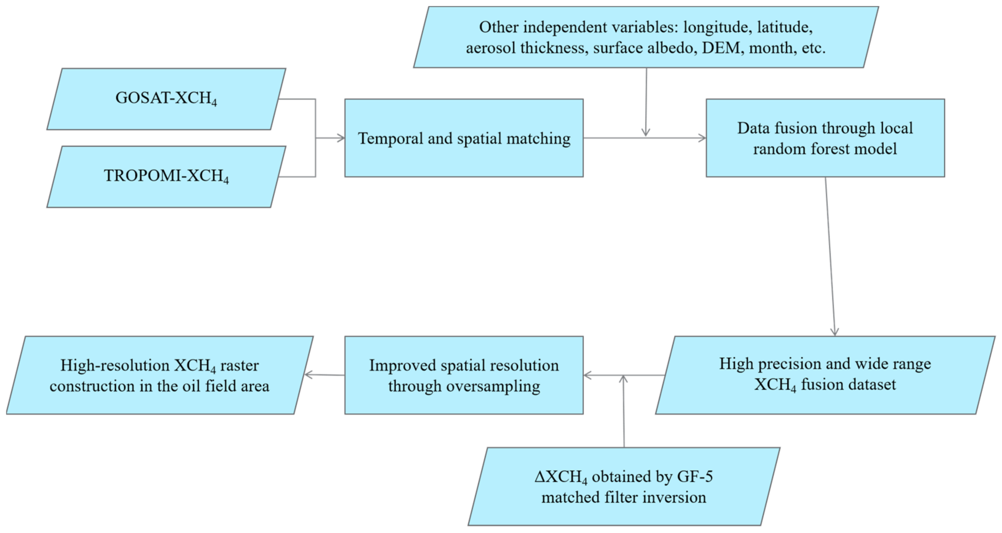
2.3. Overall Technical Approach

Upon calculation, the GOSAT data exhibit higher accuracy; however, the spatial sampling interval of the GOSAT satellite is much sparser than that of the TROPOMI instrument, thus failing to provide daily resolution with extensive XCH₄ retrieval coverage. Given the higher accuracy of GOSAT data and the broader coverage of TROPOMI data, we decided to synergize the observations from GOSAT and TROPOMI to generate improved nationwide XCH₄ data by local random forest model. The TCCON ground station XCH₄ data serve as the reference XCH₄ data and are used as the true values to measure the errors of the satellite data and the fused model data.

However, to adapt to regions with high emission backgrounds (such as oil field areas) and achieve more detailed and precise satellite remote sensing monitoring [45], the spatial resolution of the wide-coverage, high-accuracy XCH₄ dataset obtained by the LRF model fusion still does not meet monitoring requirements. We need to improve the grid resolution in specific regions. For each 7 km grid of the oil field area produced by the fusion model, we consider the results accurate. We use the GF-5 satellite as a proxy. The GF-5 satellite has a spatial resolution of 30 m, and we use matched filtering to retrieve ΔXCH₄. However, the 30 m noise is too large, so we oversample it to 1 km to match the noise scale of the fusion model. Using a regression model, we allocate the 1 km resolution ΔXCH₄ to the 7 km grid of the fusion model, generating a high-resolution, high-accuracy XCH₄ grid dataset for the oil field area. The overview of the methodology workflow is in Figure 1.

2.4. Spatial Matching

The GOSAT and Sentinel-5P satellites, as separate Earth observation platforms, possess unique design features and technical specifications, which directly impact their detection capabilities for the important greenhouse gas methane (CH₄) in the atmosphere. Firstly, there is a significant difference in spatial resolution between the two satellites [46], which determines their level of detail in capturing the distribution of CH₄ in specific regions on the ground or in the troposphere. Secondly, their methods of observing CH₄ column concentrations in the troposphere are vastly different. GOSAT uses point-column scanning, while Sentinel-5P uses swath scanning, resulting in GOSAT having a much lower coverage of CH₄ concentration compared to Sentinel-5P. These two factors together result in spatial differences in their XCH₄ data products. To carry out subsequent fusion work, we need to first manually “align” the two datasets through spatial matching, ensuring that corresponding observations from both satellites fall on the same or closely adjacent geographic grid points to obtain data suitable for fusion and to eliminate spatial differences as much as possible.

To achieve spatial matching, we use the boundaries of the grid and the interval between grid points for spatial matching [34,47]. Taking a GOSAT data point as an example, we subtract its longitude from the left boundary of the grid longitude (column number 1), and then divide by the longitude interval between grid points to determine which two longitude grid points the point falls between. Next, we observe the decimal part; if it is greater than 0.5, it indicates that the point is closer to the right-side grid point, so the right-side grid point is chosen as the longitude matching point. If it is less than 0.5, it indicates that the point is closer to the left-side grid point, so the left-side grid point is chosen as the longitude matching point. A similar process is then applied to the latitude, with the difference being that the left boundary of the longitude grid (column number 1) is the minimum longitude of the study area, whereas the upper boundary of the latitude grid (row number 1) is the maximum latitude of the study area. Therefore, the difference between the upper boundary of the latitude grid and the latitude of the point to be matched is calculated, divided by the latitude interval, and if the decimal part is greater than 0.5, it indicates that it is closer to the lower grid point, so the lower grid point is chosen as the latitude matching point; if it is less than 0.5, it indicates that it is closer to the upper grid point, so the upper grid point is chosen as the matching point. This completes the spatial matching of longitude and latitude for a GOSAT data point. By repeating these operations for each GOSAT data point, the spatial matching for all data points can be completed. The process of longitude matching for a GOSAT data point can be represented by Equation (1).

$$\begin{array}{l}n\_lon=(lonG-min\_lonT)/interval;\\ decimal\_lon=n\_lon-floor(n\_lon);\\ decimal\_lon<0.5\to lonG\leftrightarrow lonT(,floor(n\_lon)+1);\\ decimal\_lon>0.5\to lonG\leftrightarrow lonT(,ceil(n\_lon)+1);\end{array},$$

(1)

where lonG represents the longitude of the point to be matched, min_lonT represents the left boundary of the TROPOMI geographic grid (i.e., the minimum longitude of the study area, with column number 1), interval represents the interval between adjacent longitude grid points, and n_lon represents the number of intervals between the longitude of the point to be matched and the left boundary, floor() is the floor function for rounding down, decimal_lon represents the decimal part of n_lon, and ceil() is the ceiling function for rounding up.

The latitude matching process is similar.

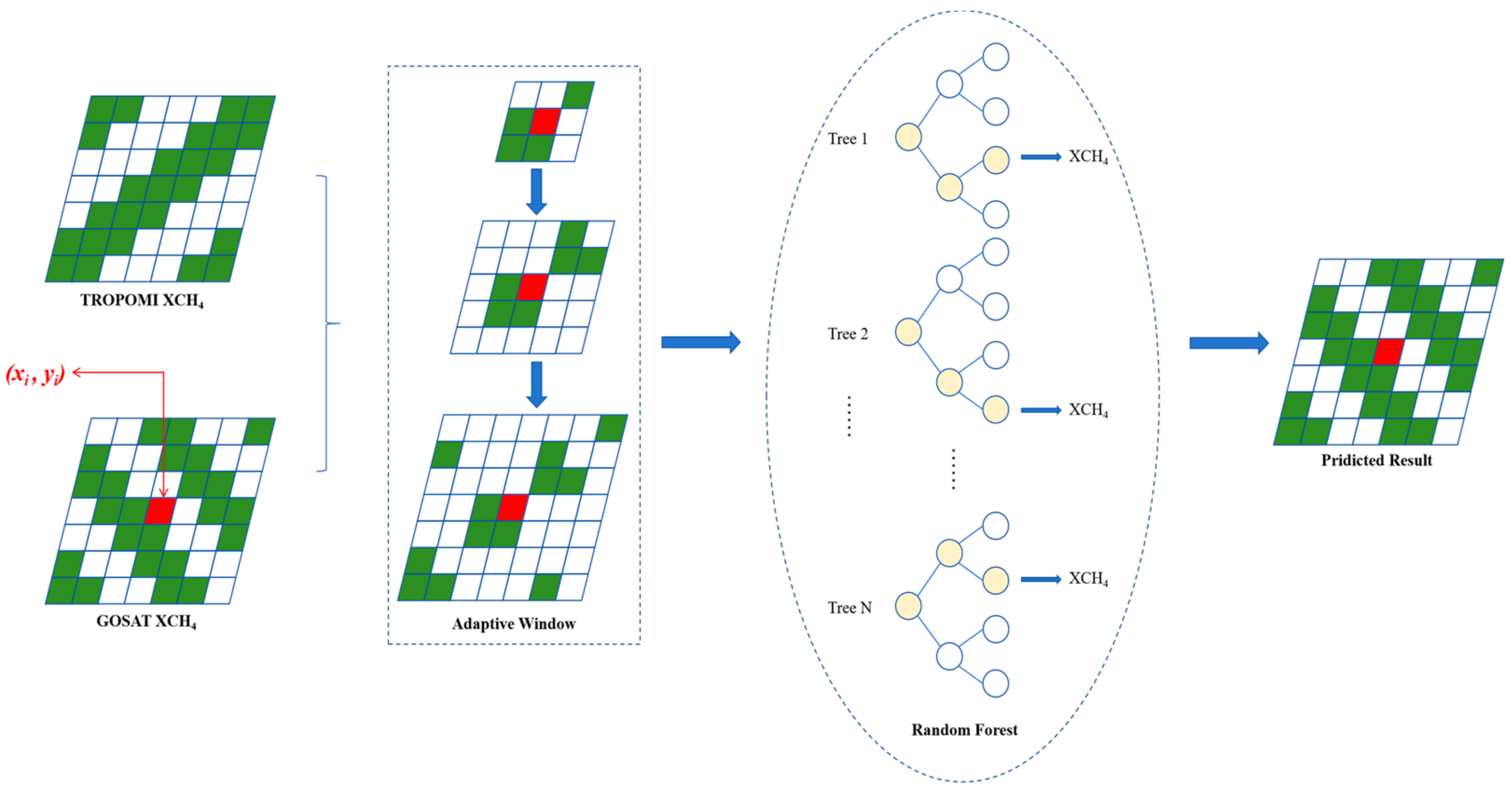
2.5. High Precision and Wide Range XCH₄ Fusion Dataset Construction

Due to variations in observation time, methods, and retrieval algorithms, there are discrepancies between the XCH₄ products from TROPOMI and GOSAT. TROPOMI offers a wide range, while GOSAT provides higher precision [48,49]. Recognizing their complementary strengths, we aim to merge these datasets to obtain an XCH₄ dataset with both high precision and broad coverage. However, directly merging them is challenging due to inherent differences, often leading to reduced accuracy. Therefore, we use GOSAT’s high-precision XCH₄ product as the reconstruction target and employ machine learning models to correct the discrepancies, enhancing TROPOMI’s precision.

Based on spatial matching, we use the local random forest (LRF) model to integrate the two satellite products. Traditional modeling methods typically employ a global model [50], which is constant across all locations and struggles to account for spatiotemporal heterogeneity, especially in a rapidly changing global environment. In contrast, our LRF model varies with spatial location, adapting to the spatiotemporal heterogeneity of global XCH₄ data distribution. The structure of the LRF model is illustrated in Figure 2.

Considering the broader coverage of TROPOMI products, during the model training process, we used GOSAT XCH4 data as the dependent variable and TROPOMI XCH4 data as the independent variable. To enhance the model’s accuracy, we also included longitude, latitude, aerosol thickness, surface albedo, DEM, and month as additional independent variables. Considering the spatial variability of missing data, we use a spatially adaptive window for model training. Assuming the number of matched samples within the window is N, the number of training samples within the window gradually increases as the window expands. Once the number of training samples within the window reaches a certain threshold (N ≥ N₀, where N₀ is set to 100 in this study), the expansion stops. Then, the samples within the window are used to train the LRF model, yielding the XCH₄ for the given location (x_i, y_i). To validate the performance of the LRF model and to ensure the proper organization of training and testing data, we employed a 5-fold cross-validation method within each local spatial window. Specifically, for each pixel (x_i, y_i) to be reconstructed, we collected matching observations from TROPOMI and GOSAT within an adaptively expanding spatial window. When the number of matching samples reached at least 100 (N ≥ N₀), where N₀ is set to 100 in this study), we stopped expanding the window to ensure sufficient data for model training and validation. We then randomly divided the collected samples into five approximately equal subsets (folds). During cross-validation, four folds (accounting for 80% of the data) were used as the training set, which included independent variables and the dependent variable. The remaining one fold (accounting for 20% of the data) was used as the test set to evaluate the predictive performance of the model. By rotating the position of the test fold in each iteration, we ensured that every data point was used for testing, enhancing the reliability of the evaluation results.

Algorithm 1 provides detailed pseudocode for the fusion of TROPOMI and GOSAT satellite data using the LRF model as employed in this work. This is intended to facilitate readers in reproducing the results by referencing Figure 2 along with the descriptions in this section.

Algorithm 1. Pseudocode for Fusion Algorithm.

Input:

- TROPOMI XCH4 dataset TTropomi

- GOSAT XCH4 dataset TGosat

- Auxiliary variables V(longitude, latitude, aerosol optical depth, surface albedo, DEM, month)

- Minimum number of training samples N0 = 100

Output:

- Reconstructed high-precision and wide-coverage XCH4 dataset Treconstructed

Procedure:

For each pixel location (xi,yi) in Ttropomi, do:

1. Initialize spatial window W centered at (xi,yi).

2. Set sample count N = 0.

3. While N < N0, do:

a. Expand spatial window W (e.g., increase radius).

b. Collect matched samples within W:

- S = {(xj,yj) | (xj,yj)∈W, TTropomi(xj,yj) and TGosat(xj,yj) are available}.

c. Update sample count.W:

4. End While

5. Prepare training data:

a. Dependent variable Y = [TGosat(xj,yj)], ∀(xj,yj)∈S.

b. Independent variables X = [ TTropomi(xj,yj), V(xj,yj)], ∀(xj,yj)∈S.

6. Train a random forest model M using X and Y.

7. Predict the XCH4 value at (xi,yi):

a. Construct input features xiinput = [TTropomi(xi,yi), V(xi,yi)].

b. Compute predicted value Ŷi = M.predict (xiinput).

8. Assign Ŷi to Trecoustructed(xi,yi).

End For

Return Trecoustructed.

2.6. Pre-Processing of GF-5 Data

Before utilizing the GF-5 imagery, it is essential to perform radiometric calibration, geometric correction, and other preprocessing steps, which are considered routine and will not be elaborated here. Additionally, it is necessary to exclude ground objects that could significantly affect the inversion results, such as clouds, shadows, and water bodies.

In this study, the cloud mask was extracted based on the cloud detection method proposed by Wang et al. [51]. This method involves calculating the equivalent apparent reflectance R₁, R₂, R₃, R₄ for each pixel in the 11th to 20th bands, 30th to 60th bands, 192nd band, and 270th to 272nd bands of the imagery. A pixel is identified as a cloud pixel if it meets the following conditions:

$$\left\{\begin{array}{l}{R}_1\cup R_2>0.3\\ R_3>0.04\cup R_1>0.15\\ {\displaystyle \frac{R_1}{R_4}}>7.5\cup {\displaystyle \frac{R_4}{R_3}}<1\end{array}\right.,$$

(2)

For shadow detection, this study employs a method based on the HSV color space. The HSV model is a hexagonal cone-shaped color space based on hue (H), saturation (S), and value (V). In this model, H represents the color information, indicating the position of the spectral color and is expressed in degrees; S represents the ratio between the selected color’s purity and its maximum possible purity; V indicates the brightness level of the color. In the HSV model, shadow regions are characterized by three main features:

• A higher hue value (H);
• High saturation (S) due to scattered light mainly originating from shorter wavelength blue-violet light;
• Lower value (V) as sunlight is blocked, reducing brightness.

Therefore, we converted the RGB image to the HSV space using Equation (3):

$$\left\{\begin{array}{l}V={\displaystyle \frac{1}{3}}(R+G+B)\\ S=1-{\displaystyle \frac{3}{R+G+B}}\min (R,G,B)\\ H=\left\{\begin{array}{l}\theta ,B\le G\\ {360}^{\circ }-\theta ,B>G\end{array}\right.\\ \theta =\arccos \left[{\displaystyle \frac{\frac{1}{2}\left|(R-G)+(R-B)\right|}{\sqrt{{(R-G)}^2+(R-B)(G-B)}}}\right]\end{array}\right.,$$

(3)

Pixels where the hue (H) and saturation (S) values exceed certain thresholds and the value (V) is below a specific threshold are identified as shadow areas.

Finally, this study uses the Normalized Difference Water Index (NDWI) to extract the water body mask, with the formula defined as

$$NDWI={\displaystyle \frac{b(Green)-b(NIR)}{b(Green)+b(NIR)}}$$

(4)

This index is calculated as the ratio of the difference between the green and near-infrared (NIR) bands to their sum. The NDWI is computed for each pixel in the image, and the pixels are then classified as water bodies based on a predefined water threshold. Pixels with an NDWI value greater than the threshold are identified as water bodies.

2.7. Construction of High-Resolution XCH₄ Fusion Dataset for Oil Fields

To obtain a high-resolution XCH₄ fusion dataset tailored to the needs of the oil and gas industry, we designed a method using ΔXCH₄ retrieved from GF-5, combined with the GFEI prior emissions inventory. We reallocate the high-precision fusion dataset output by the LRF model grid by grid in specific areas, producing a 1 km resolution XCH₄ grid product.

Based on the Beer-Lambert law, the increase in the column density of gas molecules ΔXCH₄ will affect the observed spectrum:

$$x_m(i,j)=x_r{(i,j)}_{L\times 1}\cdot e^{-k_{L\times 1}\cdot \Delta XC{H}_4(i,j)}$$

(5)

In Equation (5), x_m represents the radiance observed by the sensor, i.e., the observed spectrum; x_r represents the reference radiance; k denotes the absorption coefficient per unit gas concentration; i and j are the horizontal and vertical retrieval index coordinates in the two-dimensional hyperspectral image; and L is the length of each column in the image.

To simplify the calculations, Equation (5) is expanded to a first-order approximation using the Taylor series. Since the GF-5 AHSI sensor collects data in a column-by-column scanning mode, the inversion is performed on each column as a unit, with the mean radiance of that column approximating the reference radiance. To obtain an accurate ΔXCH_4, we solve it using the least squares method. By minimizing the weighted sum of squared residuals between each spectral band’s prior value (prior spectrum) and the observed value (observed spectrum), we can achieve the optimal estimate of the enhancement in the column density of each gas.

The log-normal distribution improves the original matched filter, i.e., LMF, addressing the issues with residuals in the conventional matched filter (MF). By taking the logarithm of both sides of Equation (5) and performing least squares operations, we obtain the LMF matched filter detector:

$$\Delta XC{H}_4={\displaystyle \frac{{(\ln (x_m(\lambda ))-\ln (x_r(\lambda )))}^T{\displaystyle {\sum }^{-1}k}}{k^T{\displaystyle {\sum }^{-1}k}}},$$

(6)

Pei et al. proposed that iterative logarithmic matched filtering allows for the updating of mean and covariance matrices, which effectively reduces the contamination of the target signal by background statistics [13]. The column density enhancement values calculated using Equation 6 are used to update the mean and covariance matrices iteratively until convergence. Outliers are considered statistically significant if they exceed twice the noise level (2σ threshold, p < 0.05). The iteration terminates either when no outliers are detected or when the number of iterations exceeds five. Subsequently, the final updated mean and covariance are used to obtain the 30 m resolution ΔXCH₄ image.

In addition, this study utilized the GFEI emissions inventory (https://dataverse.harvard.edu/dataset.xhtml?persistentId=doi:10.7910/DVN/HH4EUM&version=1.0, accessed on 1 October 2024). Developed by Harvard University, GFEI assesses methane emissions. The inventory was compared with satellite results from the Global Atmospheric Methane Observation Satellite (GOSAT) and in situ observation platform (GLOBALVIEW). GFEI uses national emissions data reported to the United Nations Framework Convention on Climate Change (UNFCCC) and maps it to infrastructure locations allocated to a 0.1° × 0.1° grid, thus creating a methane emissions map for the oil, gas, and coal industries and sub-industries.

As the spatial resolution sampling decreases, background noise becomes smoother. To adapt the ILMF inversion results to the accuracy of LRF (7 km), we upsample the 30 m resolution ΔXCH₄ image to a 1 km scale. The spatial resolution of the GFEI inventory is 0.1°, which is sampled and reprojected to a 14 km grid.

To establish the relationship between the LRF model, ILMF, and the prior GFEI, we define the convolution of the 1 km resolution ΔXCH₄ with the GFEI on a grid-by-grid basis to provide corresponding weight values for XCH₄, as described by Equation (7):

$$P_i=\Delta XC{H}_{4_i}\ast GFE{I}_i,$$

(7)

The relationship between each 1 km grid cell’s XCH_4p and the output XCH_4LRF of the LRF model can be described by the following system of equations:

$$\left\{\begin{array}{l}XC{H}_{4LRF}^1=\raisebox{1ex}{$({\beta }_1^{1}XC{H}_{4p}^1+{\beta }_2^{1}XC{H}_{4p}^2+\dots +{\beta }_{49}^{1}XC{H}_{4p}^{49})$}\!\left/ \!\raisebox{-1ex}{${\displaystyle \sum {\beta }^1}$}\right.+{\epsilon }^1\\ XC{H}_{4LRF}^2=\raisebox{1ex}{$({\beta }_1^{2}XC{H}_{4p}^1+{\beta }_2^{2}XC{H}_{4p}^2+\dots +{\beta }_{49}^{2}XC{H}_{4p}^{49})$}\!\left/ \!\raisebox{-1ex}{${\displaystyle \sum {\beta }^2}$}\right.+{\epsilon }^2\\ \dots \\ XC{H}_{4LRF}^n=\raisebox{1ex}{$({\beta }_1^{n}XC{H}_{4p}^1+{\beta }_2^{n}XC{H}_{4p}^2+\dots +{\beta }_{49}^{n}XC{H}_{4p}^{49})$}\!\left/ \!\raisebox{-1ex}{${\displaystyle \sum {\beta }^n}$}\right.+{\epsilon }^n\end{array}\right.,$$

(8)

where:

$${\beta }_i=\raisebox{1ex}{$P_i$}\!\left/ \!\raisebox{-1ex}{${\displaystyle {\sum }_{i=1}^{49}{P}_i}$}\right.,$$

(9)

To solve this model, we can consider it as a multiple linear regression process. Since this regression is rank-deficient, we use Lasso regression, which helps drive the regression coefficients towards zero, thus achieving sparsity in the features. The regression conditions are satisfied as follows:

$$argmin\left\{{\epsilon }^T\epsilon +\alpha {‖XC{H}_{4p}‖}_1\right\}$$

(10)

In Equation (10), the regularization coefficient α is introduced to control model complexity and prevent overfitting by penalizing large regression coefficients. In our study, we set α = 0.1 based on cross-validation experiments, which indicated this value achieved an optimal balance between accuracy and generalization. Specifically, we tested a range of α values and found that values below 0.1 led to overfitting, increasing error on the validation set, while values above 0.1 resulted in underfitting. Thus, α = 0.1 was selected to ensure a well-balanced trade-off between model precision and robustness.

Ultimately, while ensuring high accuracy, we produce a 1 km spatial resolution XCH₄ dataset for the oilfield region.

3. Results

Located in Shandong Province, China, Dongying is home to the Shengli Oilfield, the second-largest oil production base in the country. Consequently, this study focuses on the Dongying area. The location of Dongying within China is shown in Figure 3. The image on the left shows the location of Shandong Province within China, while the image on the right indicates the location of Dongying City within Shandong Province.

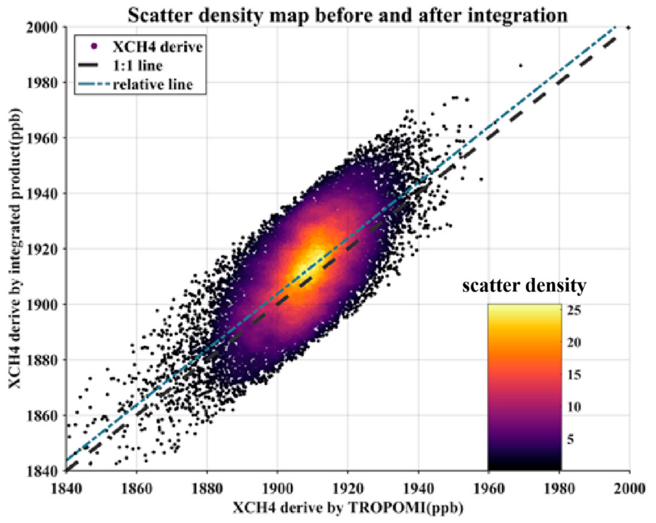
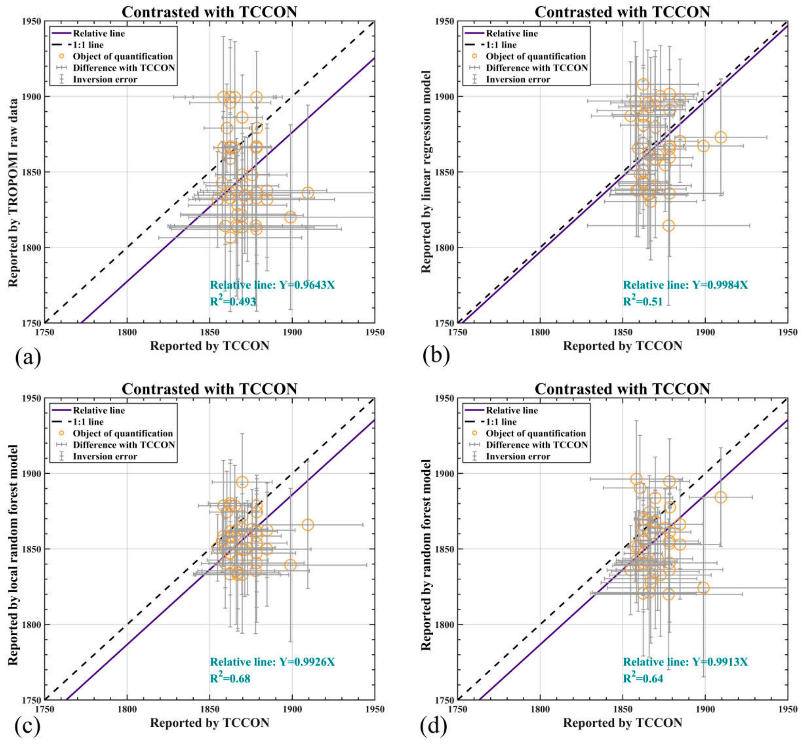
3.1. High Precision and Wide Range XCH₄ Dataset Fused by GOSAT and TROPOMI Data

After completing data filtering, spatiotemporal matching, and other preprocessing steps, we introduced independent variables such as latitude and longitude, surface albedo, and aerosol optical thickness. Using the LRF model, we fused TROPOMI and GOSAT data, combining TROPOMI’s wide coverage with GOSAT’s high precision, resulting in a high-precision global XCH₄ dataset. Figure 4 is a presentation of XCH₄ dataset fused by LRF model in Shandong Province.

We then performed a correlation fitting between the fused dataset and the pre-fusion TROPOMI product, as shown in Figure 5.

Figure 5 shows the scatter density plot for all data from 2019 to 2023 before and after fusion, processed with a 2° grid and a five-day spatial average. The overall fused values are slightly higher than the original values. The forced-through-origin fitting equation is y = 1.004x, with R² = 0.84 and RMSE = 37.116 ppb. The image and data both indicate a strong correlation between the data before and after fusion.

Furthermore, we conducted a global cross-validation of our fused products against TCCON sites. However, due to the limited number of monitoring stations in China—specifically, only the ‘Hefei’ and ‘Xianghe’ sites—we are constrained by the current density of TCCON sites and are unable to directly validate the accuracy of our fused products in regions with high oil and gas emissions. As a compromise, we utilized XCH₄ observational data from these two Chinese sites for the year 2023. We established a 20 km buffer zone around each site and conducted cross-validation by comparing the average column concentration of the LRF-fused products within the buffer zones with the observed concentrations at the sites.

Simultaneously, we employed two additional data fusion models, namely the linear regression model and the random forest model, each producing a set of fused XCH₄ products, which were also cross-validated against the TCCON sites. In addition to visual comparisons, we utilized two quantitative metrics, the coefficient of determination (R²) and root mean square error (RMSE), to evaluate the effectiveness of the models. The cross-validation results are presented in Figure 6 and

Table 2. RMSE for TROPOMI Data and Fusion Data from Three Models.

Data Source	RMSE
TROPOMI data before fusion	43.409 ppb
Data fitted by linear regression model	35.024 ppb
Data fitted by random forest model	29.118 ppb
Data fitted by local random forest model	23.201 ppb

. Figure 6 compares the original TROPOMI XCH₄ data and the XCH₄ products derived from the three different fusion models against the TCCON site data. Specifically, Figure 6a–d show the cross-validation images for the original data, the linear regression model, the local random forest model, and the random forest model, respectively, along with the corresponding R² values.

Table 2 presents the RMSE values for the pre-fusion data and the fused products compared to the TCCON site data.

As shown in Figure 6 and Table 2, upon calculation, our LRF model achieved an R² of 0.68, higher than the standard random forest model (0.64) and the linear regression model (0.51). The RMSE between the fused product and TCCON ground station data is 23.201 ppb, lower than the standard random forest model (29.118 ppb) and linear regression model (35.024 ppb), indicating that the LRF model’s fusion is superior. Additionally, the RMSE of the product obtained by the LRF model is significantly lower than before fusion (43.409 ppb), demonstrating that data fusion effectively improves product accuracy and reduces error. However, while the fused XCH₄ dataset inherits both the wide coverage of TROPOMI and the high accuracy of GOSAT, its resolution still does not meet the requirements for oil field monitoring. Therefore, we further enhanced the resolution in the oil field regions based on the high-precision, wide-coverage XCH₄ dataset obtained.

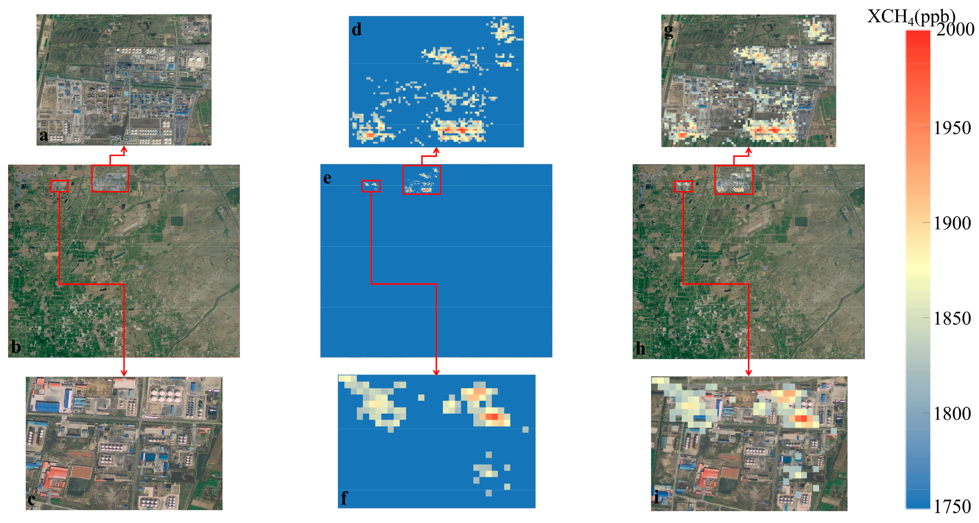
3.2. High-Resolution ΔXCH₄ Retrieval from GF-5 in the Oil Field Area

Within the study area, we first filtered and preprocessed the GF-5 satellite images. Initially, we applied cloud masking, shadow masking, and water masking to remove false positive features, thereby eliminating their interference with the retrieval results. Subsequently, we applied a matched filter operator to the study area to obtain 30-m high-resolution ΔXCH₄ values. Figure 7 presents a representative matched filtering result for a typical section of our study area. This figure shows the temporally averaged results from multiple observations by the GF-5 satellite over the oilfield region on June 20. In the process of matched filtering, we need to average the retrieval results from multiple scenes of GF-5 imagery to obtain the final result. This is because single-scene imagery has a transient nature, and methane emission sources identified from a single scene may not represent persistent sources. Averaging the retrieval results from multiple scenes helps identify continuous emission sources, allowing us to focus on these persistent sources in future work and improve both the efficiency and effectiveness of our efforts. Figure 7b provides the satellite base map for the displayed area, while Figure 7a,c focus on two specific industrial sites within the region. Figure 7e shows the matched filtering results for the entire area, and Figure 7d,f present the results for the two industrial sites. In Figure 7h, the matched filtering results are overlaid onto the satellite base map, with areas lacking XCH₄ enhancement (less than 20 ppb increase) set to null. Figure 7g,i display the overlay results and base map images for the two industrial sites. It is evident from the combined analysis of Figure 7a,c,g,i that XCH₄ levels are significantly elevated in the oil and gas industrial areas, particularly in the regions surrounding oil storage tanks. Pronounced methane plumes were observed in the GF-5 imagery after matched filtering. The average XCH₄ enhancement in the oil tank areas reached 176.24 ppb in Figure 7a and 201.33 ppb in Figure 7c. Other parts of the industrial sites, excluding the oil tank areas, showed enhancements of approximately 100 ppb. As seen in Figure 7e, following the masking steps to remove false positives, there is almost no XCH₄ enhancement in the areas outside the industrial sites.

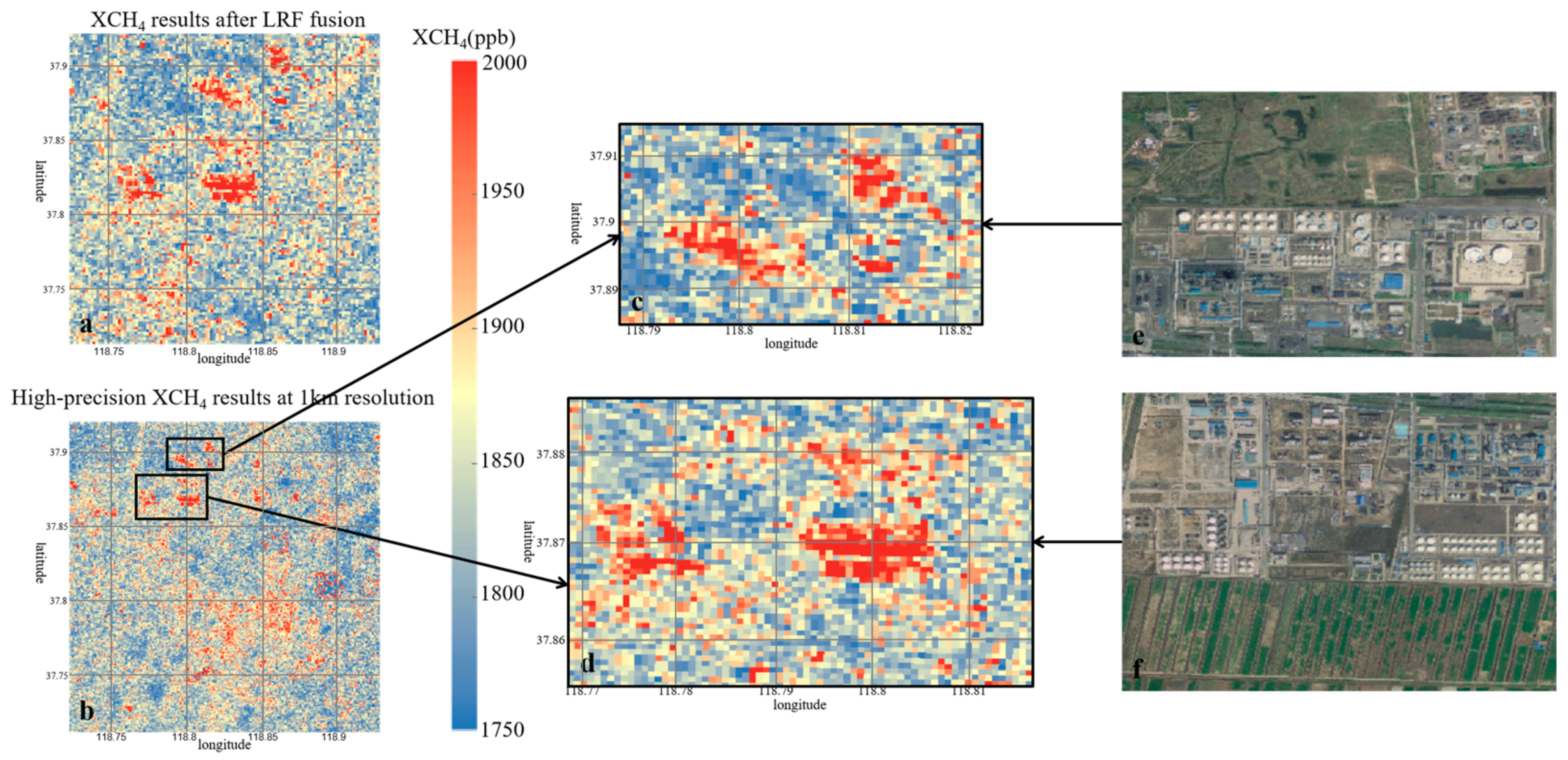
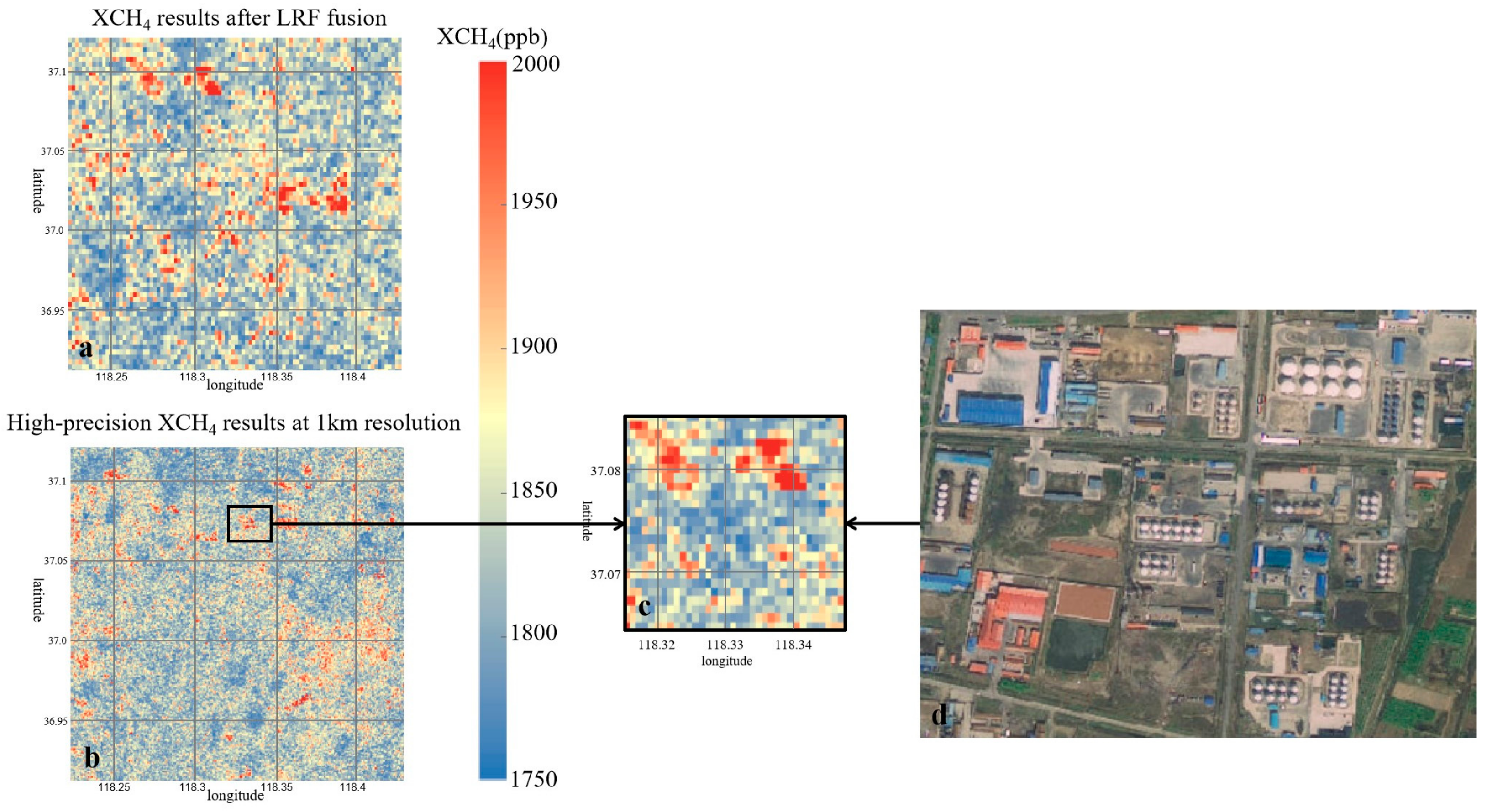
3.3. Construction of High-Resolution XCH₄ Products for the Oil Field Area and Comparison of High- and Low-Resolution Datasets

In the previous sections, we generated a 7 km resolution, high-precision XCH₄ product using the LRF model. Simultaneously, we fused data from hyperspectral satellites such as GF-5, employing a matched filtering method to obtain 30 m high-resolution ΔXCH₄ data for the oilfield regions. Based on these two datasets, we upsampled the 30 m resolution ΔXCH₄ dataset to a 1 km resolution and resampled the 0.1° resolution GFEI inventory to a 7 km resolution. Subsequently, using the Lasso regression algorithm introduced in Section 2.7, we divided each 7 km resolution high-precision XCH₄ grid into 49 independent subgrid units, generating a denser grid allocation framework. We then redistributed the XCH₄ within each 7 km grid to its corresponding subgrids, resulting in a high-precision, high-resolution XCH₄ gridded dataset for the oilfield areas.

The final 1 km resolution XCH₄ grid fused both top-down and bottom-up methane observation and accounting approaches, integrating the bottom-up GFEI inventory and the top-down GF-5 satellite observations within the high-precision XCH₄ grid generated by the LRF model. Figure 8 illustrates a case study of our fusion algorithm applied to an oilfield region in Dongying. Figure 8a displays the high-precision, low-resolution XCH₄ dataset for a portion of the study area derived from the LRF model, while Figure 8b shows the 1 km resolution XCH₄ dataset for the same area. From Figure 8a,b, it is evident that, although some high-concentration methane distribution areas can be identified in the 7 km resolution XCH₄ image, more precise attribution is challenging at this resolution. This is particularly true for concentration enhancements caused by pipeline leaks or strong point source emissions, which cannot be finely attributed at the 7 km resolution.

Figure 8c,d provide magnified views of the XCH₄ grid after fusing the high-resolution GF-5 data in two specific areas of the Shengli Oilfield, and their corresponding satellite maps are shown in Figure 8e,f, respectively. At the 1 km resolution, it becomes much easier to spatially attribute methane column concentration enhancements. For example, in Figure 8c, at longitude 118.41 and latitude 37.88, the 1 km resolution grid clearly resolves the strong enhancement region seen in the 7 km resolution grid of Figure 8a, along with five weaker enhancements that correspond to the background enhancements within the black box in Figure 8a. In Figure 8d, a significant methane plume is identified at longitude 118.41 and latitude 37.83. According to imagery from Google Earth, this coordinate corresponds to a major methane emission source in the oilfield, where methane column concentration enhancement reached 312.3 ppb. In contrast, the corresponding 7 km grid in Figure 8a shows an enhancement of 181.5 ppb (the average concentration of all grids within the rectangle was taken as the background methane column concentration for this region). Our calculations indicate that 93% of the enhancement in this 7 km grid is due to the plume generated by this major emission source, consistent with accounting metrics provided by the oilfield company. However, due to the confidentiality of the data, we cannot provide detailed metrics in this paper. In our previous work, leveraging collaboration with the company, we conducted field verification in the region and observed a broad area of slight enhancement northeast of the emission source, corresponding to the pipeline transport area and oil tank storage area of the industrial complex.

In order to illustrate the correctness of the results of this study, another case study of an oil field area in Dongying was chosen for presentation, as shown in Figure 9. Again, Figure 9a shows the high-precision, low-resolution XCH₄ dataset generated by the LRF model for part of the study area, while Figure 9b shows the 1-km-resolution XCH₄ dataset for the same area. It is still difficult to more accurately attribute the areas of high methane concentration distribution identified in the 7 km resolution XCH₄ images. At 1 km resolution, however, spatial attribution of enhanced methane column concentrations becomes easier. For example, a distinct methane plume appears in the region shown in zoom in Figure 9c. According to Google Earth imagery, this coordinate corresponds to the main methane emission source in the oil field, with a methane column concentration enhancement of 295.26 ppb. In contrast, the corresponding 7 km grid in Figure 9a shows an enhancement of 164.33 ppb (the average concentration of all grids within the rectangle is considered as the background methane column concentration in this region). Our calculations indicate that 85% of the enhancement in this 7 km grid is due to the plume from this major emission source, which is also consistent with the accounting metrics provided by the oil companies. However, due to the confidentiality of the data, we are also unable to provide detailed metrics in this paper. However, even with the 1 km resolution imagery, it remains challenging to attribute minor XCH₄ enhancements caused by facility-level emissions. We advocate for the future development of XCH₄ datasets with even finer spatial resolution.

4. Discussion

4.1. Strengths and Weaknesses of Each Model

In this study, we utilized three models to fuse GOSAT and TROPOMI data: the linear regression model, the random forest model, and the local random forest (LRF) model. The linear regression model is favored for its simplicity, ease of interpretation, and high computational efficiency. However, it is highly sensitive to outliers and lacks the capacity to effectively describe and predict complex data relationships. In contrast, the random forest model mitigates the impact of noise and outliers by averaging the results from multiple decision trees, thereby minimizing the influence of any single outlier on the overall prediction. This enhances the model’s robustness and accuracy, enabling it to capture nonlinear relationships within the data. Consequently, we decided to discard the linear regression model.

Building upon the random forest model, we incorporated an advanced method from the literature: the local random forest (LRF) model. This model adapts to spatial variability, making it particularly well-suited for addressing the spatiotemporal heterogeneity in the global distribution of XCH₄ data. After cross-validating with TCCON sites, we calculated the coefficient of determination (R²) and the root mean square error (RMSE) between the fused products and TCCON site data for each model. As anticipated, the LRF model exhibited the highest R² and the lowest RMSE, consistent with our expectations. Therefore, we selected the fused products from the LRF model as the high-precision, wide-coverage XCH₄ dataset for further research.

4.2. Challenge and Forward

The development of high-resolution XCH₄ datasets through multi-source satellite fusion presents significant opportunities for advancing methane monitoring and emission control in the oil and gas industry. However, this process is fraught with several challenges. The heterogeneity of data sources—stemming from variations in spatial resolution, temporal coverage, and spectral response among different satellites—introduces considerable complexity into the data fusion process. This complexity necessitates the development of sophisticated algorithms capable of integrating diverse datasets while maintaining high accuracy and consistency. Additionally, the challenge of spatiotemporal matching, due to differences in satellite observation times and orbits, poses a critical issue that can lead to inconsistencies and gaps in the fused datasets, affecting their reliability.

The computational demands associated with processing high-resolution data further complicate the task, requiring substantial resources and advanced computational techniques to perform detailed matched filtering and redistribution operations over large areas. Moreover, the uncertainty inherent in model selection and optimization adds another layer of difficulty, as different models may yield varying results depending on their approach to data handling, making it challenging to ensure that the models accurately reflect real-world conditions. Compounding these issues is the scarcity of ground-based validation data, particularly in regions with high oil and gas emissions, where the limited distribution of TCCON and other ground stations hampers the ability to robustly assess the accuracy of satellite-derived products.

Looking ahead, advances in multi-source data fusion algorithms and the deployment of next-generation hyperspectral satellites are expected to significantly improve the spatiotemporal resolution and coverage of XCH₄ datasets. The development of advanced machine learning techniques, such as deep learning and transfer learning, can enhance the capability to integrate diverse satellite datasets more effectively. These algorithms can learn complex patterns and relationships between different data sources, enabling more accurate and reliable XCH₄ datasets. On the satellite technology front, upcoming missions like NASA’s MethaneSAT and the European Space Agency’s Sentinel-5P and future Sentinel-5 satellites promise higher resolution and more frequent observations of methane concentrations globally. These satellites are equipped with advanced sensors that offer improved spectral and spatial resolution, significantly enhancing the precision of methane monitoring efforts. Collaboration with international methane monitoring networks will also be crucial. Integrating satellite observations with data from ground-based networks like the Total Carbon Column Observing Network (TCCON) and incorporating measurements from drones and aircraft can fill spatial and temporal gaps in satellite data. This integration provides high-resolution local observations essential for identifying emission hotspots and validating satellite-derived products.

These developments will enhance the capacity for real-time methane monitoring, particularly in oil and gas regions. The integration of satellite data with ground-based observations, drones, and aircraft will also provide richer validation datasets, further increasing the reliability and precision of the fused products. Global collaboration and data sharing will be crucial in establishing standardized and unified XCH₄ datasets, which can be applied across various sectors beyond the oil and gas industry, including agriculture and waste management. Such datasets will be instrumental in supporting global efforts to monitor and reduce methane emissions, contributing to broader climate change mitigation strategies. As technology continues to advance and collaborative efforts expand, the construction of high-resolution XCH₄ datasets through multi-source satellite fusion will play an increasingly pivotal role in achieving global carbon reduction goals. By leveraging enhanced fusion algorithms, next-generation satellites, and comprehensive observational networks, the research community can significantly contribute to global efforts aimed at reducing methane emissions and combating climate change. As technology continues to advance and collaborative efforts expand, the construction of high-resolution XCH₄ datasets through multi-source satellite fusion will play an increasingly pivotal role in achieving global carbon reduction goals.

5. Conclusions

5.1. Data Sources and Data Processing

In this study, XCH₄ data acquired from TROPOMI and GOSAT satellites between 2019 and 2023 were systematically analyzed. GOSAT data are known for their high accuracy, while TROPOMI data are known for their wide coverage. In order to combine the advantages of both, we constructed a global XCH₄ dataset with both high accuracy and wide coverage. Before constructing the model, we performed spatiotemporal matching of the two datasets to ensure high spatiotemporal correlation of the training data.

5.2. Model Development and Performance Evaluation

We used a linear regression model, a random forest model, and a localized random forest model designed to effectively integrate data from GOSAT and TROPOMI. We quantitatively assessed the integration effectiveness of each model through the coefficient of determination (R²) and root mean square error (RMSE). The results showed that the localized random forest model performed well in terms of R² value (0.68) and RMSE value (23.201 ppb) and thus was selected as the best fusion model to achieve the construction of a high-precision and wide-coverage XCH₄ dataset.

5.3. High-Resolution Data Processing

For high-emission background areas (e.g., oil field areas), in order to achieve more detailed and precise satellite remote sensing purposes, proxy data from GF-5 satellites were utilized, and ΔXCH₄ data were acquired by matched filtering technique, which successfully improved the resolution to 1 km. Subsequently, the lasso regression method was used to integrate the ΔXCH₄ data with 1-km resolution into the fusion model of a 7-km grid, and a high-resolution and high-precision XCH₄ grid dataset of the oilfield area was generated.

5.4. Significance of the Research Results

The oilfield XCH₄ dataset developed in this research not only achieves a high level of accuracy and resolution but also provides strong support for optimizing methane monitoring in the oilfield region and controlling domestic carbon emissions. The research results of this dataset are of great practical value in advancing China’s goal of carbon peaking and carbon neutrality and have a very positive contribution to environmental protection and climate change response.

References

1. Denman, K.L. Contribution of working group I to the fourth assessment report of the intergovernmental panel on climate change. In Climate Change 2007: The Physical Science Basis; IPOC: Geneva, Switzerland, 2007; Volume 7. [Google Scholar]
2. Han, G.; Huang, Y.; Shi, T.; Zhang, H.; Li, S.; Zhang, H.; Chen, W.; Liu, J.; Gong, W. Quantifying CO2 emissions of power plants with Aerosols and Carbon Dioxide Lidar onboard DQ-1. Remote Sens. Environ. 2024, 313, 114368. [Google Scholar] [CrossRef]
3. Saunois, M.; Stavert, A.R.; Poulter, B.; Bousquet, P.; Zhuang, Q. The Global Methane Budget 2000–2017. Earth Syst. Sci. Data 2020, 12, 1561–1623. [Google Scholar] [CrossRef]
4. Shindell, D.; Kuylenstierna, J.C.; Vignati, E.; van Dingenen, R.; Amann, M.; Klimont, Z.; Anenberg, S.C.; Muller, N.; Janssens-maenhout, G.; Raes, F.; et al. Simultaneously Mitigating Near-Term Climate Change and Improving Human Health and Food Security. Science 2012, 335, 183–189. [Google Scholar] [CrossRef] [PubMed]
5. Lauvaux, T.; Lauvaux, T.; Giron, C.; Mazzolini, M.; d’Aspremont, A.; Duren, R.; Cusworth, D.; Shindell, D.; Ciais, P. Global assessment of oil and gas methane ultra-emitters. Science 2022, 375, 557–561. [Google Scholar] [CrossRef]
6. Peng, S.; Lin, X.; Thompson, R.L.; Xi, Y.; Liu, G.; Hauglustaine, D.; Lan, X.; Poulter, B.; Ramonet, M.; Saunois, M.; et al. Wetland emission and atmospheric sink changes explain methane growth in 2020. Nature 2022, 612, 477–482. [Google Scholar] [CrossRef]
7. Naus, S.; Maasakkers, J.D.; Gautam, R.; Omara, M.; Stikker, R.; Veenstra, A.K.; Nathan, B.; Irakulis-Loitxate, I.; Guanter, L.; Pandey, S.; et al. Assessing the Relative Importance of Satellite-Detected Methane Superemitters in Quantifying Total Emissions for Oil and Gas Production Areas in Algeria. Environ. Sci. Technol. 2023, 57, 19545–19556. [Google Scholar] [CrossRef]
8. Han, G.; Pei, Z.; Shi, T.; Mao, H.; Li, S.; Mao, F.; Ma, X.; Zhang, X.; Gong, W. Unveiling Unprecedented Methane Hotspots in China’s Leading Coal Production Hub: A Satellite Mapping Revelation. Geophys. Res. Lett. 2024, 51, e2024GL109065. [Google Scholar] [CrossRef]
9. He, T.-L.; Boyd, R.J.; Varon, D.J.; Turner, A.J. Increased methane emissions from oil and gas following the Soviet Union’s collapse. Proc. Natl. Acad. Sci. USA 2024, 121, e2314600121. [Google Scholar] [CrossRef]
10. Chen, Y.L.; Sherwin, E.D.; Berman, E.S.; Jones, B.B.; Gordon, M.P.; Wetherley, E.B.; Kort, E.A.; Brandt, A.R. Quantifying Regional Methane Emissions in the New Mexico Permian Basin with a Comprehensive Aerial Survey. Environ. Sci. Technol. 2022, 56, 4317–4323. [Google Scholar] [CrossRef]
11. Irakulis-Loitxate, I.; Guanter, L.; Liu, Y.N.; Varon, D.J.; Maasakkers, J.D.; Zhang, Y.; Chulakadabba, A.; Wofsy, S.C.; Thorpe, A.K.; Duren, R.M.; et al. Satellite-based survey of extreme methane emissions in the Permian basin. Sci. Adv. 2021, 7, eabf4507. [Google Scholar] [CrossRef]
12. Varon, D.J.; McKeever, J.; Jervis, D.; Maasakkers, J.D.; Pandey, S.; Houweling, S.; Aben, I.; Scarpelli, T.; Jacob, D. Satellite Discovery of Anomalously Large Methane Point Sources from Oil/Gas Production. Geophys. Res. Lett. 2019, 46, 13507–13516. [Google Scholar] [CrossRef]
13. Pei, Z.; Han, G.; Mao, H.; Chen, C.; Shi, T.; Yang, K.; Ma, X.; Gong, W. Improving quantification of methane point source emissions from imaging spectroscopy. Remote Sens. Environ. 2023, 295, 113652. [Google Scholar] [CrossRef]
14. Lavoie, T.N.; Shepson, P.B.; Gore, C.A.; Stirm, B.H.; Kaeser, R.; Wulle, B.; Lyon, D.; Rudek, J. Assessing the Methane Emissions from Natural Gas-Fired Power Plants and Oil Refineries. Environ. Sci. Technol. 2017, 51, 3373–3381. [Google Scholar] [CrossRef] [PubMed]
15. Cusworth, D.H.; Duren, R.M.; Thorpe, A.K.; Olson-Duvall, W.; Heckler, J.; Chapman, J.W.; Eastwood, M.L.; Helmlinger, M.C.; Green, R.O.; Asner, G.P.; et al. Intermittency of Large Methane Emitters in the Permian Basin. Environ. Sci. Technol. Lett. 2021, 8, 567–573. [Google Scholar] [CrossRef]
16. Sherwin, E.D.; Rutherford, J.S.; Zhang, Z.; Chen, Y.; Wetherley, E.B.; Yakovlev, P.V.; Berman, E.S.F.; Jones, B.B.; Cusworth, D.H.; Thorpe, A.K.; et al. US oil and gas system emissions from nearly one million aerial site measurements. Nature 2024, 627, 328–334. [Google Scholar] [CrossRef]
17. Williams, J.P.; Omara, M.; Himmelberger, A.; Zavala-Araiza, D.; MacKay, K.; Benmergui, J.; Sargent, M.; Wofsy, S.C.; Hamburg, S.P.; Gautam, R. Small emission sources disproportionately account for a large majority of total methane emissions from the US oil and gas sector. EGUsphere 2024, 2024, 1–31. [Google Scholar] [CrossRef]
18. Wu, D.; Yue, Y.; Jing, J.; Liang, M.; Sun, W.; Han, G.; Lou, M. Background Characteristics and Influence Analysis of Greenhouse Gases at Jinsha Atmospheric Background Station in China. Atmosphere 2023, 14, 1541. [Google Scholar] [CrossRef]
19. Jacob, D.J.; Varon, D.J.; Cusworth, D.H.; Dennison, P.E.; Frankenberg, C.; Gautam, R.; Guanter, L.; Kelley, J.; McKeever, J.; Ott, L.E.; et al. Quantifying methane emissions from the global scale down to point sources using satellite observations of atmospheric methane. Atmos. Chem. Phys. 2022, 22, 9617–9646. [Google Scholar] [CrossRef]
20. Zhang, Y.; Gautam, R.; Pandey, S.; Omara, M.; Maasakkers, J.D.; Sadavarte, P.; Lyon, D.; Nesser, H.; Sulprizio, M.P.; Varon, D.J.; et al. Quantifying methane emissions from the largest oil-producing basin in the United States from space. Sci. Adv. 2020, 6, eaaz5120. [Google Scholar] [CrossRef]
21. Pei, Z.P.; Han, G.; Ma, X.; Shi, T.Q.; Gong, W. A Method for Estimating the Background Column Concentration of CO2 Using the Lagrangian Approach. IEEE Trans. Geosci. Remote Sens. 2022, 60, 4108112. [Google Scholar] [CrossRef]
22. Zhang, J.; Han, G.; Mao, H.; Pei, Z.; Ma, X.; Jia, W.; Gong, W. The Spatial and Temporal Distribution Patterns of XCH4 in China: New Observations from TROPOMI. Atmosphere 2022, 13, 177. [Google Scholar] [CrossRef]
23. Song, H.; Sheng, M.; Lei, L.; Guo, K.; Zhang, S.; Ji, Z. Spatial and Temporal Variations of Atmospheric CH4 in Monsoon Asia Detected by Satellite Observations of GOSAT and TROPOMI. Remote Sens. 2023, 15, 3389. [Google Scholar] [CrossRef]
24. Huang, Y.Y.; Han, G.; Shi, T.Q.; Li, S.W.; Mao, H.Q.; Nie, Y.H.; Gong, W. FI-SCAPE: A Divergence Theorem Based Emission Quantification Model for Air/Space-Borne Imaging Spectrometer Derived XCH4 Observations. IEEE J. Sel. Top. Appl. Earth Obs. Remote Sens. 2024. [CrossRef]
25. Breiman, L. Random forests. Mach. Learn. 2001, 45, 5–32. [Google Scholar] [CrossRef]
26. Kump, L.R. What drives climate? Nature 2000, 408, 651–652. [Google Scholar] [CrossRef]
27. Glumb, R.; Davis, G.; Lietzke, C. The TANSO-FTS-2 instrument for the GOSAT-2 greenhouse gas monitoring mission. In Proceedings of the 2014 IEEE Geoscience and Remote Sensing Symposium, Quebec City, QC, Canada, 13–18 July 2014; IEEE: New York, NY, USA, 2014; pp. 1238–1240. [Google Scholar]
28. Varon, D.J.; Jacob, D.J.; Hmiel, B.; Gautam, R.; Lyon, D.R.; Omara, M.; Sulprizio, M.; Shen, L.; Pendergrass, D.; Nesser, H.; et al. Continuous weekly monitoring of methane emissions from the Permian Basin by inversion of TROPOMI satellite observations. Atmos. Chem. Phys. Discuss. 2022, 23, 7503. [Google Scholar] [CrossRef]
29. Plant, G.; Kort, E.A.; Murray, L.T.; Maasakkers, J.D.; Aben, I. Evaluating urban methane emissions from space using TROPOMI methane and carbon monoxide observations. Remote Sens. Environ. 2022, 268, 112756. [Google Scholar] [CrossRef]
30. Schneising, O.; Buchwitz, M.; Reuter, M.; Vanselow, S.; Bovensmann, H.; Burrows, J.P. Remote sensing of methane leakage from natural gas and petroleum systems revisited. Atmos. Chem. Phys. 2020, 20, 9169–9182. [Google Scholar] [CrossRef]
31. Li, K.; Bai, K.; Jiao, P.; Chen, H.; He, H.; Shao, L.; Sun, Y.; Zheng, Z.; Li, R.; Chang, N.B. Developing unbiased estimation of atmospheric methane via machine learning and multiobjective programming based on TROPOMI and GOSAT data. Remote Sens. Environ. 2024, 304, 114039. [Google Scholar] [CrossRef]
32. Yang, J.; Gan, R.; Luo, B.; Wang, A.; Shi, S.; Du, L. An Improved Method for Individual Tree Segmentation in Complex Urban Scene Based on Using Multispectral LiDAR by Deep Learning. IEEE J. Sel. Top. Appl. Earth Obs. Remote Sens. 2024, 17, 6561–6576. [Google Scholar] [CrossRef]
33. Wang, Y.; Yuan, Q.; Li, T.; Yang, Y.; Zhou, S.; Zhang, L. Seamless mapping of long-term (2010–2020) daily global XCO2 and XCH4 from the Greenhouse Gases Observing Satellite (GOSAT), Orbiting Carbon Observatory 2 (OCO-2), and CAMS global greenhouse gas reanalysis (CAMS-EGG4) with a spatiotemporally self-supervised fusion method. Earth Syst. Sci. Data 2023, 15, 3597–3622. [Google Scholar]
34. Qiu, R.; Han, G.; Li, X.; Xiao, J.; Liu, J.; Wang, S.; Li, S.; Gong, W. Contrasting responses of relationship between solar-induced fluorescence and gross primary production to drought across aridity gradients. Remote Sens. Environ. 2024, 302, 113984. [Google Scholar] [CrossRef]
35. Xu, M.; Han, G.; Pei, Z.; Yu, H.; Li, S.; Gong, W. Advanced method for compiling a high-resolution gridded anthropogenic CO2 emission inventory at a regional scale. Geo-Spat. Inf. Sci. 2024, 1–14. [Google Scholar]
36. Liu, B.; Ma, X.; Guo, J.; Wen, R.; Li, H.; Jin, S.; Ma, Y.; Guo, X.; Gong, W. Extending the wind profile beyond the surface layer by combining physical and machine learning approaches. Atmos. Chem. Phys. 2024, 24, 4047–4063. [Google Scholar] [CrossRef]
37. Liang, A.; Pang, R.; Chen, C.; Xiang, C. XCO2 Fusion Algorithm Based on Multi-Source Greenhouse Gas Satellites and CarbonTracker. Atmosphere 2023, 14, 1335. [Google Scholar] [CrossRef]
38. Shi, T.; Han, G.; Ma, X.; Pei, Z.; Chen, W.; Liu, J.; Zhang, X.; Li, S.; Gong, W. Quantifying strong point sources emissions of CO2 using spaceborne LiDAR: Method development and potential analysis. Energy Convers. Manag. 2023, 292, 117346. [Google Scholar] [CrossRef]
39. He, J.; Wang, W.; Fu, M.; Wang, Y. Insights into global visibility patterns: Spatiotemporal distributions revealed by satellite remote sensing. J. Clean. Prod. 2024, 468, 143069. [Google Scholar] [CrossRef]
40. Cai, M.; Han, G.; Ma, X.; Pei, Z.; Gong, W. Active–passive collaborative approach for XCO2 retrieval using spaceborne sensors. Opt. Lett. 2022, 47, 4211–4214. [Google Scholar] [CrossRef]
41. Zhang, H.; Han, G.; Chen, W.; Pei, Z.; Liu, B.; Liu, J.; Zhang, T.; Li, S.; Gong, W. Validation Method for Spaceborne IPDA LIDAR XCO2 Products via TCCON. IEEE J. Sel. Top. Appl. Earth Obs. Remote Sens. 2024, 17, 16984–16992. [Google Scholar] [CrossRef]
42. Wang, L.; Yang, L.; Wang, Y. Analysis of China’s Oil and Gas Industrial Green and Low-carbon Development Strategies and Paths in New Era. Pet. Sci. Technol. Forum 2022, 42, 67. [Google Scholar]
43. Liang, A.; Gong, W.; Han, G.; Xiang, C. Comparison of Satellite-Observed XCO2 from GOSAT, OCO-2, and Ground-Based TCCON. Remote Sens. 2017, 9, 1033. [Google Scholar] [CrossRef]
44. Pei, Z.; Han, G.; Shi, T.; Ma, X.; Gong, W. A XCO2 Retrieval Algorithm Coupled Spatial Correlation for the Aerosol and Carbon Detection Lidar. Atmos. Environ. 2023, 309, 119933. [Google Scholar] [CrossRef]
45. Shi, T.Q.; Han, G.; Ma, X.; Gong, W.; Chen, W.; Liu, J.; Zhang, X.; Pei, Z.; Gou, H.; Bu, L. Quantifying CO2 Uptakes Over Oceans Using LIDAR: A Tentative Experiment in Bohai Bay. Geophys. Res. Lett. 2021, 48, e2020GL091160. [Google Scholar] [CrossRef]
46. Qiu, R.; Li, X.; Han, G.; Xiao, J.; Ma, X.; Gong, W. Monitoring drought impacts on crop productivity of the US Midwest with solar-induced fluorescence: GOSIF outperforms GOME-2 SIF and MODIS NDVI, EVI, and NIRv. Agric. For. Meteorol. 2022, 323, 109038. [Google Scholar] [CrossRef]
47. Pei, Z.; Han, G.; Ma, X.; Su, H.; Gong, W. Response of major air pollutants to COVID-19 lockdowns in China. Sci. Total Environ. 2020, 743, 140879. [Google Scholar] [CrossRef] [PubMed]
48. Zhang, H.; Han, G.; Ma, X.; Chen, W.; Zhang, X.; Liu, J.; Gong, W. Robust algorithm for precise X CO2 retrieval using single observation of IPDA LIDAR. Opt. Express 2023, 31, 11846–11863. [Google Scholar] [CrossRef]
49. Lorente, A.; Borsdorff, T.; Butz, A.; Hasekamp, O.; Aan De Brugh, J.; Schneider, A.; Wu, L.; Hase, F.; Kivi, R.; Wunch, D.; et al. Methane retrieved from TROPOMI: Improvement of the data product and validation of the first 2 years of measurements. Atmos. Meas. Tech. 2021, 14, 665–684. [Google Scholar] [CrossRef]
50. Ying, J.; Jiang, J.; Wang, H.; Liu, Y.; Gong, W.; Liu, B.; Han, G. Analysis of the Income Enhancement Potential of the Terrestrial Carbon Sink in China Based on Remotely Sensed Data. Remote Sens. 2023, 15, 3849. [Google Scholar] [CrossRef]
51. Yi, J.; Huang, Y.; Pei, Z.; Han, G. Urban Area Observing System (UAOS) Simulation Experiment Using DQ-1 Total Column Concentration Observations. EGUsphere 2024, 2024, 1–40. [Google Scholar]
Figure 1. Overview of the methodology workflow in this study.
Applsci 14 11100 g001
Figure 2. Structure of the LRF model.
Applsci 14 11100 g002
Figure 3. Location of the study area (Dongying, Shandong Province, China).
Applsci 14 11100 g003
Figure 4. Presentation of XCH4 dataset fused by LRF model in Shandong Province.
Applsci 14 11100 g004
Figure 5. Scatter Density Plot of Fused Data vs. Original TROPOMI Data, with the Black Dashed Line Representing the 1:1 Line and the Blue Dashed Line Representing the Fitted Line.
Applsci 14 11100 g005
Figure 6. Comparison and fitting plots of pre-merger and post-merger data with TCCON station data for each model, where (a) shows the pre-merger TROPOMI data compared to the TCCON station data, (b) represents the linear regression model, (c) represents the localized random forest model, and (d) represents the random forest model.
Applsci 14 11100 g006
Figure 7. Example of ΔXCH4 Retrieval Results, where (b) is a satellite map of the region, (a,c) are zoomed presentations of the plant area in (b); (e) is a map of the matched filter results of the region, and (d,f) are zoomed presentations of the same region as in (a,c); (h) is a display of the matched filter results superimposed on the satellite map and hiding the background values, and (g,i) are zoomed presentations of the plant area in (h).
Applsci 14 11100 g007
Figure 8. High-resolution and high-precision XCH4 dataset for oilfield regions. (a) shows the low-resolution data of a region after the fusion of the LRF model, (b) shows the high-resolution data of the same region, (c,d) are zoomed presentations of the two high-emission plant areas in (b), and (e,f) are satellite maps corresponding to the areas presented in (c) and (d), respectively.
Applsci 14 11100 g008
Figure 9. High-resolution and high-precision XCH4 dataset for oilfield regions. (a) shows the low-resolution data of an area different from Figure 8 after LRF model fusion, (b) shows the high-resolution data of the same area, (c) shows a zoomed-in display of a high-emission plant area in (b), and (d) is a satellite map corresponding to the area displayed in (c).
Applsci 14 11100 g009