Optimization of Stope Structural Parameters for Steeply Dipping Thick Ore Bodies: Based on the Simulated Annealing Algorithm

Abstract

Stope structural parameters are of great significance for the safe production of mines. To efficiently and safely mine steeply dipping ultra-thick ore bodies, the K. Kegel strength design formula and limit analysis method were used to calculate a reasonable range of stope parameters. Considering the actual mining conditions, the mechanical responses under different structural parameters were obtained through numerical simulations based on a central composite experimental design. A regression model for maximum tensile stress, maximum compressive stress, and maximum vertical displacement was established using the second-order response surface method. The regression model was then used as the objective function, and multi-objective optimization was performed using a simulated annealing algorithm to obtain the Pareto optimal solution set. Based on practical engineering needs, a stope span of 15.0 m, a pillar width of 10.0 m, and a roof thickness of 11.9 m were determined as the optimal structural parameters, achieving a balance between safety and economic efficiency.

1. Introduction

Underground mining is gradually becoming the primary method of extraction for mines, with increasingly prominent challenges. Compared to open-pit mining, the complex geological environment, variable mining conditions, and numerous risk factors significantly impact the safety of underground mining. Under the influence of multiple factors, rationally setting stope structural parameters is crucial for maintaining the stability of mined-out areas [1,2]. On one hand, it enhances stope stability and reduces the risk of safety accidents such as roof falls and wall collapses. On the other hand, it improves the ore recovery rates and the economic efficiency of the mine, contributing to the sustainable development of mineral resources. Therefore, the study of optimizing stope structural parameters is of great significance in the mining process [3].

Based on the research and analysis of stope structural parameter optimization both domestically and internationally, commonly used methods include the Mathew stability chart method and the FLAC3D numerical simulation method for optimizing stope structural parameters, as well as multi-objective optimization methods [4,5,6]. The Mathew stability chart method is primarily used to estimate the exposed area of the stope roof and the exposed area of the filling body sidewalls. This evaluation method introduces various correction factors and, based on rock mass quality grading, comprehensively considers multiple on-site influencing factors to perform a multi-criteria assessment of the actual engineering. The FLAC3D numerical simulation method [7,8] has a wide range of applications and can simulate various mechanical behaviors of three-dimensional soils, rock masses, and other materials under stress conditions. It is commonly used to optimize stope span, stope length, and stage height parameters. However, it is less effective when discussing issues such as the exposed area of the filling body sidewalls. Numerical simulation analysis enables the use of finite difference software for three-dimensional modeling of complex ore bodies and stopes, ensuring efficient analysis of complex spatial stability. However, numerical simulation analysis primarily focuses on assessing the mechanical characteristics of stopes, often overlooking economic benefits to ensure stope stability. Therefore, multi-objective optimization of stope parameters is the key to addressing this issue [9,10,11]. Optimizing stope structural parameters typically involves adjusting stope dimensions, such as roof thickness, pillar width, and stope span. This process usually requires analyzing the relationship between these dimensions and their mechanical responses.

Multi-objective optimization methods involve using optimization-based mathematical models combined with numerical simulation software to optimize stope structural parameters. Given that stope structural parameters are influenced by multiple factors, multi-objective optimization overcomes the limitations of single-objective optimization focused solely on mechanical responses by incorporating economic factors such as cost, ensuring both economic and safe production in mining. Liu [12] and others constructed a neural network model based on factors such as pillar thickness and pillar interface dimensions. They used chaotic optimization methods and ANSYS finite element numerical simulation software to determine stope structural parameters under different technical mining conditions to ensure safe ore recovery and also improve ore recovery rates. KePing Z [13] and others used numerical analysis software to determine the safety factors for parameter combinations within a selected range. They utilized these safety factors as training samples for a BP neural network to model the nonlinear relationship between parameter combinations and safety factors. This approach aimed to find the optimal solution for the fitness function and the corresponding parameter combination. Given the high computational complexity of multi-objective optimization problems, heuristic algorithms are generally more efficient for solving them [14,15]. Heuristic algorithms [16,17,18,19] are a class of algorithms based on intuition or empirical construction that provide feasible solutions to combinatorial optimization problems within an acceptable time. Common heuristic algorithms include genetic algorithms [20,21], ant colony algorithms [22,23], simulated annealing algorithms [24,25], and neural networks. Matamoros [26] and others proposed a three-stage stochastic optimization model considering grade uncertainty and used genetic algorithms combined with numerical simulation software to determine the optimal parameters for stope, maximizing mining profits. Saghatforoush combined neural networks with ant colony optimization algorithms to optimize blasting parameters, reducing the occurrence probability of flyrock and secondary blasting [27]. Li Jianguo improved the simulated annealing algorithm to optimize parking space allocation efficiency indicators, verifying the effectiveness of the improved simulated annealing algorithm in reducing energy consumption and increasing garage operating profits [28].

This paper employs response surface methodology to identify stope span, pillar width, roof thickness, and ore recovery rate as key influencing factors. Central composite experiments are conducted to investigate the impact of these factors on stope stability and ore recovery rate. Regression models for stope tensile strength, compressive strength, and displacement are developed using response surface methodology. An optimization of stope structural parameters is performed using an algorithm combining simulated annealing and Pareto optimization [29,30,31], resulting in reasonable stope structural parameters. This has significant practical implications for safe, economical, and efficient mining.

2. Materials and Methods

2.1. Materials

The topography of a certain limestone mine in Nandan County, Guangxi, is characterized by steep slopes, with nearby basic farmland. The ore body is relatively thick and exposed at the surface, making the mining conditions complex. To protect forest land and the basic farmland, the mining operator proposes using segmented drilling and blasting with a stope method. Choosing appropriate stope structural parameters is a key technical challenge for achieving efficient and safe mining. The mining elevation for the limestone ore is between +1060 m and +830 m, with underground mining employed and the ore type being limestone. The ore body is located within the F1 fault zone with a nearly southwest–northeast strike, a strike length of 720 m, a length of nearly 1800 m, and a surface exposure width of 40–70 m. The average thickness of the ore body is 65.31 m, with a dip angle of approximately 65°. Based on the mining technical conditions and current status of the limestone mining area, and drawing on experiences from mining thick ore bodies, the design for the limestone mining area will use the segmented drilling and blasting stope method as the main mining approach. The layout of the stope is shown in Figure 1.

The stope is arranged along the vertical strike of the ore body, with a stage height of 50 m and a sublevel height of 20 m. The ore block length corresponds to the horizontal thickness of the ore body, the stope width is 15 m, the pillar width is 12 m, and the roof thickness is 11 m. An external vein preparation method is used, with the ramp, stage haulage drifts, and sublevel drifts arranged outside the footwall rock movement line of the ore body. The ramp connects the upper- and lower-stage haulage drifts and the sublevel drilling drifts, while the ore pass crosscut connects the along-vein stage haulage drift with the hanging wall return air drift. At the bottom of each ore block, an ore pass crosscut is arranged, with a loading road spaced approximately every 10 m along one side of the crosscut. A trench drift is arranged at the bottom of the stope. A sublevel drilling drift is driven 20–25 m above the stage haulage drift. A cutting drift and cutting raise are driven near the ore–rock interface on the sublevel drilling horizon, using a CKY50 drill to drill upward, parallel, medium-depth holes in the cutting drift. The cutting raise serves as a free face for blasting, forming a cutting slot. Ore extraction from the stope starts with the cutting slot as the free face, where fan-shaped holes are drilled upward using a CKY50 drill from the sublevel drilling drift. The blast hole diameter is 65 mm, with a minimum resistance line of 1.2–1.6 m. All blast holes are drilled before blasting, with 3–5 rows of holes grouped for each blast. Blasting must not allow the lower sublevel to advance ahead of the upper sublevel; instead, the upper and lower sublevels should maintain a vertical face or allow the upper sublevel to advance by one row of blast holes. After the ore is blasted, it falls by gravity into the trench drift at the bottom of the stope. The ore is loaded by a loader into an ore pass spaced 10 m apart along the loading road and discharged into nearby ore passes. Rock samples from the mining area are processed and used for laboratory rock mechanics experiments to obtain mechanical parameters, and the Hoek–Brown criterion is used to reduce rock strength, yielding the rock mechanics parameters, as shown in

Table 1. Rock mass mechanical parameters.

Rock Type	Tensile Strength σt/MPa	Compressive Strength σc/MPa	Elastic Modulus Em/GPa	Cohesion Cm/KPa	Friction Angle φ (°)	Density γ/g/cm3	Poisson’s Ratio
Ore Body	0.341	5.973	8.867	1086	48.90	2.65	0.23
Limestone	3.063	37.342	24.75	6122	52.80	2.70	0.21

.

2.2. Methods

2.2.1. Pillar Stability Calculation

Stability calculations are performed using the K. Kegel strength calculation formula [32].

$${\sigma }_p={\sigma }_C\times B\times \sqrt{{\displaystyle \frac{w}{H}}}$$

(1)

Here, σ_p—pillar strength, MPa; σ_c—rock’s uniaxial compressive strength, MPa; w—pillar width, m; H—pillar height, m; and B—fissure factor, whose value ranges from 0.4 to 1.0, typically taken as 0.7. When using the K. Kegel strength design formula, the safety factor of the pillar is

$$F={\displaystyle \frac{{\sigma }_C\times B\times \sqrt{\frac{w_0}{H}}}{\gamma \times h\times \left(1+\frac{w_0}{w_P}\right)}}$$

(2)

Here, σ_c—rock’s uniaxial compressive strength; B—fissure factor; $w_0$—average width of the stope; H—pillar height; $\gamma$—rock mass density; h—mining depth; and $w_p$—pillar width.

Substituting the parameters into the above formula yields the safety factors corresponding to different pillar widths, as shown in

Table 2. Safety factors for different pillar widths.

	Pillar Width	10 m	11 m	12 m	13 m	14 m
Stope Span
15 m		1.276	1.416	1.553	1.689	1.823
16 m		1.235	1.372	1.507	1.641	1.772
17 m		1.196	1.330	1.464	1.595	1.725
18 m		1.16	1.292	1.423	1.553	1.681
19 m		1.127	1.256	1.385	1.513	1.640
20 m		1.096	1.223	1.35	1.476	1.601

.

Since the pillar must support a long-term load to maintain the stability of the stope, the allowable safety factor should be greater than 1. Therefore, the average stope span is 15–20 m, and the pillar width is 10–14 m.

2.2.2. Roof Stability Calculation

The formula for calculating the safe thickness of the roof based on the limit analysis method is as follows:

$${\left[{\displaystyle \frac{M_p}{q}}\right]}^{1/2}=\left\{\begin{array}{c}{\displaystyle \frac{L\sqrt{{\left(C_{n}L\right)}^2+3l}-C_n{L}^2}{\sqrt{3}Cl}}{\displaystyle \frac{1}{CL}}<{\left[{\displaystyle \frac{M_p}{q}}\right]}^{1/2}\le {\displaystyle \frac{\sqrt{3}}{CL}}\\ \left[{\displaystyle \frac{l\sqrt{l^2+3C_n^2{L}^2}-l^2}{\sqrt{3}C{C}_n^{2}L}}\right]{\left[{\displaystyle \frac{M_p}{q}}\right]}^{1/2}\ge {\displaystyle \frac{\sqrt{3}}{CL}}\end{array}\right.$$

(3)

Here, q is the distributed load on the roof, in MPa, and M_p is the unit limit moment, which comprehensively reflects factors such as the rock properties and thickness of the roof, calculated as follows [33]:

$$M_P={\displaystyle \frac{1}{6}}{\sigma }_t{h}^2$$

(4)

Here, h is the roof thickness, in meters (m); σ_t is the tensile strength of the roof rock layer, in MPa; L is the length of the working face, in meters (m); l is the span of the working face, in meters (m); and C and C_n are equivalent coefficients, with their values under different boundary conditions shown in

Table 3. Values of C and C_n under different boundary conditions.

Boundary Constraint Forms	C	Cn
Four-edge fixed slab	4	1
Three-sided fixed and one-sided simply supported	2 + $\sqrt{2}$	$4/(2+\sqrt{2})$

[33].

The distributed load on the roof is q = 30 m × 2.66 t/m³ = 79.8 t/m², The parameters required for calculating the safe thickness of the roof rock layer according to the boundary constraint forms in Table 3 are shown in

Table 4. Parameters for calculating roof safety thickness.

Equivalent Coefficient C	Equivalent Coefficient Cn	Stope Length L (m)	Stope Span L (m)	Roof Tensile Strength (MPa)	Roof Rock Bulk Density (KN/m3)	(Boundary Constraint Forms)
4	1	65	15–20	0.501	26.5	Four-edge fixed slab
3.414	1.172	65	15–20	0.501	26.5	Three-sided Fixed and one-sided simply supported

.

The relationship between the roof safety thickness and the stope span of the working face under different stope spans (15–20 m) with a stope length of 65 m is shown in

Table 5. Relationship between roof safety thickness and stope span.

(m)	15	16	17	18	19	20	Boundary Constraint Forms
Roof Safety Thickness (m)	10.13	10.71	11.28	11.84	12.39	12.93	Four-edge fixed slab
	11.08	11.72	12.35	12.06	12.97	13.58	Three-sided fixed and one-sided simply supported

.

Based on the calculations above, the stope span should be 15–20 m, the pillar width should be 10–14 m, and the roof thickness should be 10–14 m.

2.3. Numerical Simulation Experiment

2.3.1. Basic Assumptions and Initial Geostress Field

Based on the actual geological engineering conditions of the limestone mine, the following assumptions are made [34,35]:

Rock Mass Assumptions: The rock mass is assumed as an ideal elastoplastic material. Beyond the yield point, with plastic flow, the material’s strength and volume remain unchanged, and rock strain hardening or softening is not considered.

Material Properties: The rock mass is considered homogeneous and isotropic, with plastic flow not affecting the material’s isotropy.

Limitations of Finite Difference Calculations: It is assumed there is no influence from tectonic activity within the site. The initial rock stress is considered as a geostatic field, with inter-layer contacts assumed to be integrative and internal rock layers treated as continuous media.

Numerical Model: A numerical model is established based on the occurrence of the ore body and rock mass, with limestone being the dominant rock type and the ore body primarily consisting of calcite. The gravity field is taken as the initial rock stress field. The vertical and horizontal movements at the model’s base are restricted. The lateral pressure coefficients on the four sides are automatically calculated by the program according to Poisson’s ratio, with the overlying rock layer’s load being its self-weight.

2.3.2. Model Construction and Calculation Results

To study the impact of various parameters on stope stability, the model was appropriately simplified. The rock mechanics parameters used in the numerical simulation in this article are those listed in Table 1. Assuming an average ore body thickness of 65 m and a surface dip angle of 65°, and based on Saint Venant’ s principle, the excavation range was set to 3–5 times the model boundary, with dimensions of 90 m in length, 400 m in width, and 350 m in height. The finite element type is three-dimensional hexahedral, with the number of nodes per element being 3, the number of degrees of freedom per node being 2, and a total of 38,912 elements and 7959 nodes. The mesh type is triangular, with a mesh size of 4. The computer system used for numerical simulation is a PC, and the numerical simulation method employed is the finite element method, as shown in Figure 2. For stope spans of 15–20 m, pillar widths of 10–14 m, and roof thicknesses of 10–14 m, 15 test points were designed for numerical simulation analysis according to the central composite design principle. The stope parameters, as well as the horizontal and numerical calculation results, are shown in

Table 6. Comparison of mechanical response indicators for each scheme.

Experimental Schemes	Stope Span /m	Pillar Span /m	Roof Thickness /m	Maximum Tensile Stress/Mpa	Maximum Compressive Stress/Mpa	Maximum Vertical Displacement/mm
1	15	10	10	0.183	4.873	4.154
2	15	10	14	0.238	4.662	4.665
3	15	12	12	0.198	4.886	4.126
4	15	14	10	0.243	4.299	3.728
5	15	14	14	0.204	4.636	3.810
6	17.5	10	12	0.293	5.245	4.898
7	17.5	12	10	0.296	5.009	4.424
8	17.5	12	12	0.297	4.910	4.829
9	17.5	12	14	0.259	4.675	4.613
10	17.5	14	12	0.316	5.225	4.002
11	20	10	10	0.308	5.421	5.090
12	20	10	14	0.292	5.120	5.249
13	20	12	12	0.330	5.191	4.646
14	20	14	10	0.388	5.180	4.363
15	20	14	14	0.337	5.365	4.278

.

The numerical analysis results indicate that after excavation of the stope, the maximum principal stress is tensile, while the minimum principal stress is compressive, mainly concentrated at the center of the roof and the pillar. Among the analyzed schemes, the maximum tensile stress is 0.388 MPa and the maximum compressive stress is 5.768 MPa, both of which are within the limits of the rock mass tensile strength (0.341 MPa) and compressive strength (5.973 MPa). The maximum vertical displacement of the stope is 5.249 mm. Thus, the stress and displacement of the stope in the above schemes are within reasonable ranges, and no damage has occurred to the stope.

2.4. Response Surface Methodology

Based on the calculation results of the stope parameters from Table 6, a response surface model is established for the relationships between the stope span X₁, pillar span X₂, roof thickness X₃, maximum tensile stress Y₁, maximum compressive stress Y₂, and maximum vertical displacement Y₃. To improve the accuracy of the response surface model, a second-order nonlinear response surface model is used to map the relationships between the stope parameters and each mechanical response. The basic expression of the model is as follows [36]:

$$\widehat{y}=f\left(x_1,x_2,\dots ,x_n\right)=a_0+\sum _{i=1}^n{a}_i{x}_i+\sum _{i=1}^n{a}_{ii}{x}_i^2+\sum _{i=1}^{n-1}\sum _{j=i+1}^n{a}_{ij}{x}_i{x}_j$$

(5)

Here, $\widehat{y}$ is the approximated response coefficient; a₀, a_i, a_ii, and a_ij (i = 1, 2,…, n; j = 1, 2, …, n) are the coefficients to be determined; and x_i represents the random variables (e.g., stope span, pillar span, and roof thickness). Using the least squares method and MATLAB R2023a software, the unbiased estimates of the coefficients a₀, a_i, a_ii, and a_ij are determined.

For the fitting of the three response surface models, the resulting models are as follows:

$$\begin{array}{c}{Y}_1=-1.5304+0.14849x_1-0.090238x_2+0.13829x_3-0.0037067x_1^2+0.0043333x_2^2-\\ 0.0024167x_3^2+0.002475x_1{x}_2-0.002075{x_{1}x}_3-0.0040312x_2{x}_3\end{array}$$

(6)

$$\begin{array}{c}{Y}_2=6.7801+0.16224x_1-1.6968x_2+1.0459x_3-0.0044x_1^2+0.04225x_2^2-\\ 0.056x_3^2+0.0151x_1{x}_2-0.00605{x_{1}x}_3+0.032313x_2{x}_3\end{array}$$

(7)

$$\begin{array}{c}{Y}_3=-11.5338+1.0938x_1+0.5934x_2+0.46357x_3-0.019636x_1^2-0.014681x_2^2+\\ 0.0024444x_3^2-0.010425x_1{x}_2-0.012975{x_{1}x}_3-0.021031x_2{x}_3\end{array}$$

(8)

The coefficient of determination (R²) reflects the goodness of fit of the model. For the quadratic response surface models described in Equations (10) to (12), which include interaction terms, the R² values are as follows:

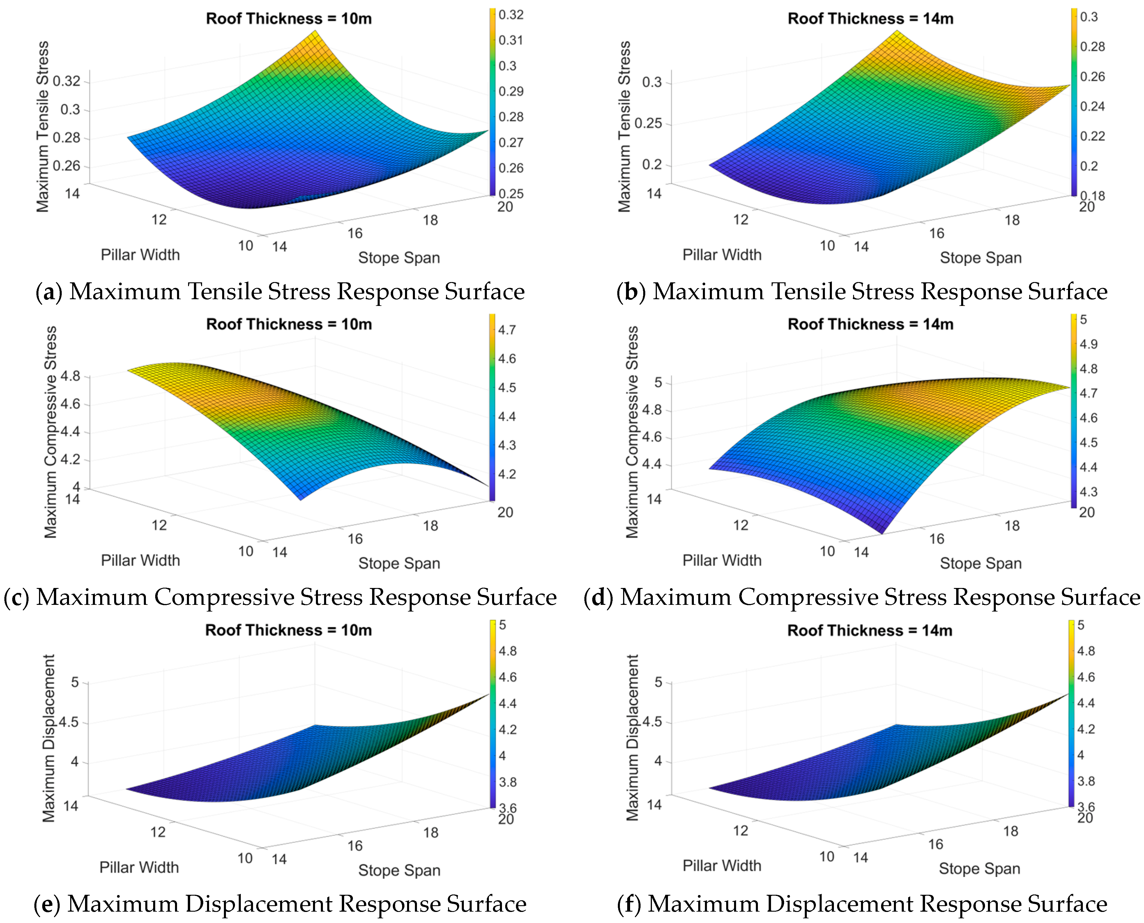
• Maximum Tensile Stress (Y₁): R² = 0.98.
• Maximum Compressive Stress (Y₂): R² = 0.91.
• Maximum Vertical Displacement (Y₃): R² = 0.96.

These R² values indicate a good fit of the response surface models to the data [37,38], suggesting that the models are well-suited to meet the needs of practical engineering applications. The regression models Y₁, Y₂, and Y₃ indicate that the stope span, pillar span, and roof thickness have significant effects on the compressive stress, tensile stress, and displacement in the stope.

In Figure 3a,b, it can be observed that when the roof thickness is 10 m and 14 m, there is a positive correlation between the maximum tensile stress and the stope span, meaning that as the stope span increases, the maximum tensile stress also increases. Additionally, with the increase in pillar span, the maximum tensile stress first decreases and then increases. Figure 3c,d show that when the roof thickness is 10 m, the maximum compressive stress exhibits a negative correlation with both the stope span and pillar span, meaning that the maximum compressive stress decreases as both the pillar span and stope span increase. However, when the roof thickness is fixed at 14 m, the compressive stress decreases with an increase in pillar span but increases with an increase in stope span. Figure 3e,f illustrate that the maximum displacement of the stope shows a positive correlation with both the stope span and pillar span, meaning that the displacement increases with the stope span and pillar span and also increases with the roof thickness. The relationships between different variables are explained in points 1, 2, 3, and 4 below.

• Effect of Stope Span on Compressive and Tensile Stresses in the Stope: As the stope span increases, the stability of the surrounding rock gradually decreases, weakening the load-bearing capacity of the roof and causing a redistribution of stresses above the stope. A larger span increases tensile stress in the middle of the roof, potentially triggering bending and tensile effects, similar to the “arching effect” in structural mechanics. With a larger span, stress concentrates in the central region, increasing tensile stress, especially in rock structures where cracks and fractures are more likely to form, leading to stress concentration. As the span grows, the roof’s load-bearing capacity further diminishes, reducing overall stiffness and increasing compressive stress in the support zones. Larger spans also lead to compressive stress concentration near the center and support points, potentially causing local stress instability and rock failure. In general, the greater the span, the more likely bending and collapse occur in the roof, increasing maximum compressive stress and reducing structural stability overall.
• Effects of Pillar Width on Compressive and Tensile Stress in the Stope: When the pillar width is small, the support strength and stiffness of the pillar are insufficient to effectively resist the self-weight of the roof and external loads, leading to significant deformation of the roof and concentration of tensile stress in certain areas. As the size of the pillar increases, their load-bearing capacity and stiffness improve, allowing for better resistance against roof subsidence and deformation, which in turn reduces the deflection of the roof and the tensile stress resulting from that deflection. However, when the pillar reaches a critical size, the support strength exhibits a saturation effect, and further increases in pillar size yield minimal improvement in load-bearing capacity. At the same time, the increase in the weight of the pillar causes the roof to bear greater downward forces, thereby increasing tensile stress in the roof. When the pillar width is small, the support effect is relatively good, resulting in a more uniform distribution of compressive stress in the roof. However, as the pillar width increases, the support capacity gradually weakens, leading to the concentration of compressive stress near the support points and increasing the risk of localized compressive stress. When the pillar width reaches its critical size, the support stiffness is significantly insufficient, causing further increases in compressive stress in the central area of the roof, which may trigger local instability and rock failure.
• Effects of Roof Thickness on Compressive and Tensile Stress: Thicker roofs possess greater stiffness, enabling them to better resist bending deformation and reduce the concentration of tensile stress, particularly diminishing the tensile effects in the central region of the roof. Consequently, thick roofs can effectively distribute tensile stress under support conditions, lowering the risk of structural instability. In contrast, thinner roofs have lower stiffness, making them more susceptible to larger bending and tensile stress concentrations, which increases the risk of fissures and cracking in the central area. Additionally, the increased stiffness of thicker roofs helps to minimize stope deformation and decrease compressive stress concentrations, resulting in a more uniform distribution of maximum compressive stress and an overall reduction in compressive stress.
• Effects of Stress on Stope Displacement: In the stope, the distribution of stress directly affects displacement. As the support conditions or external loads change, an increase in stress within the stope can lead to greater plastic deformation of the rock mass, resulting in increased displacement.

It is evident that there are complex interactions between the variables, making the optimization of a single model of limited significance [39,40]. To enhance economic benefits and ensure safe mining operations, it is necessary to consider the relationship between various structural parameters and mechanical properties comprehensively and implement multi-objective optimization.

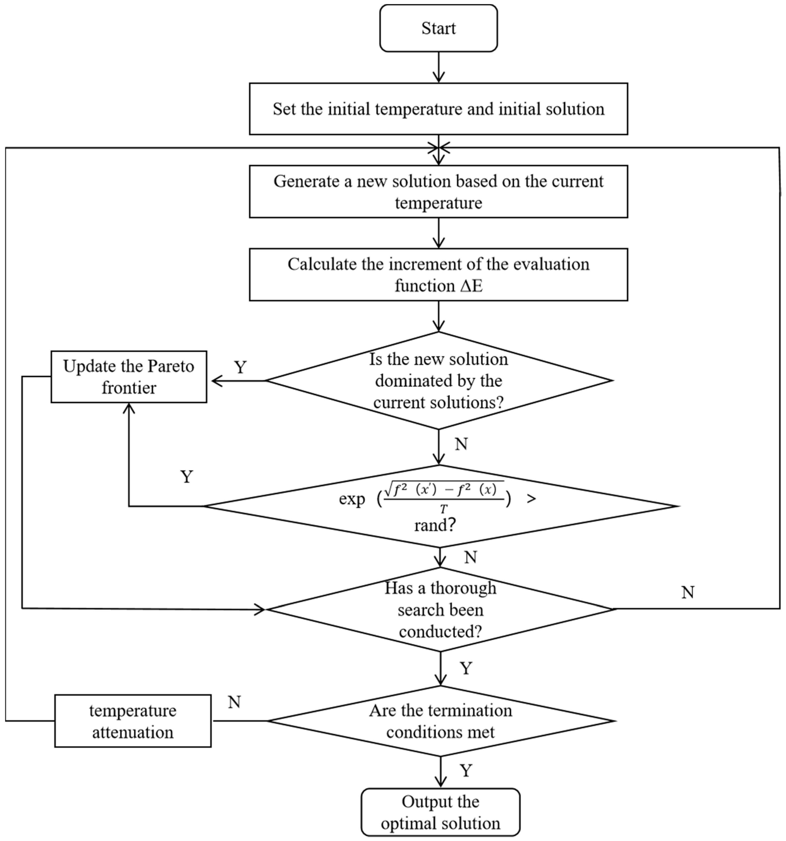
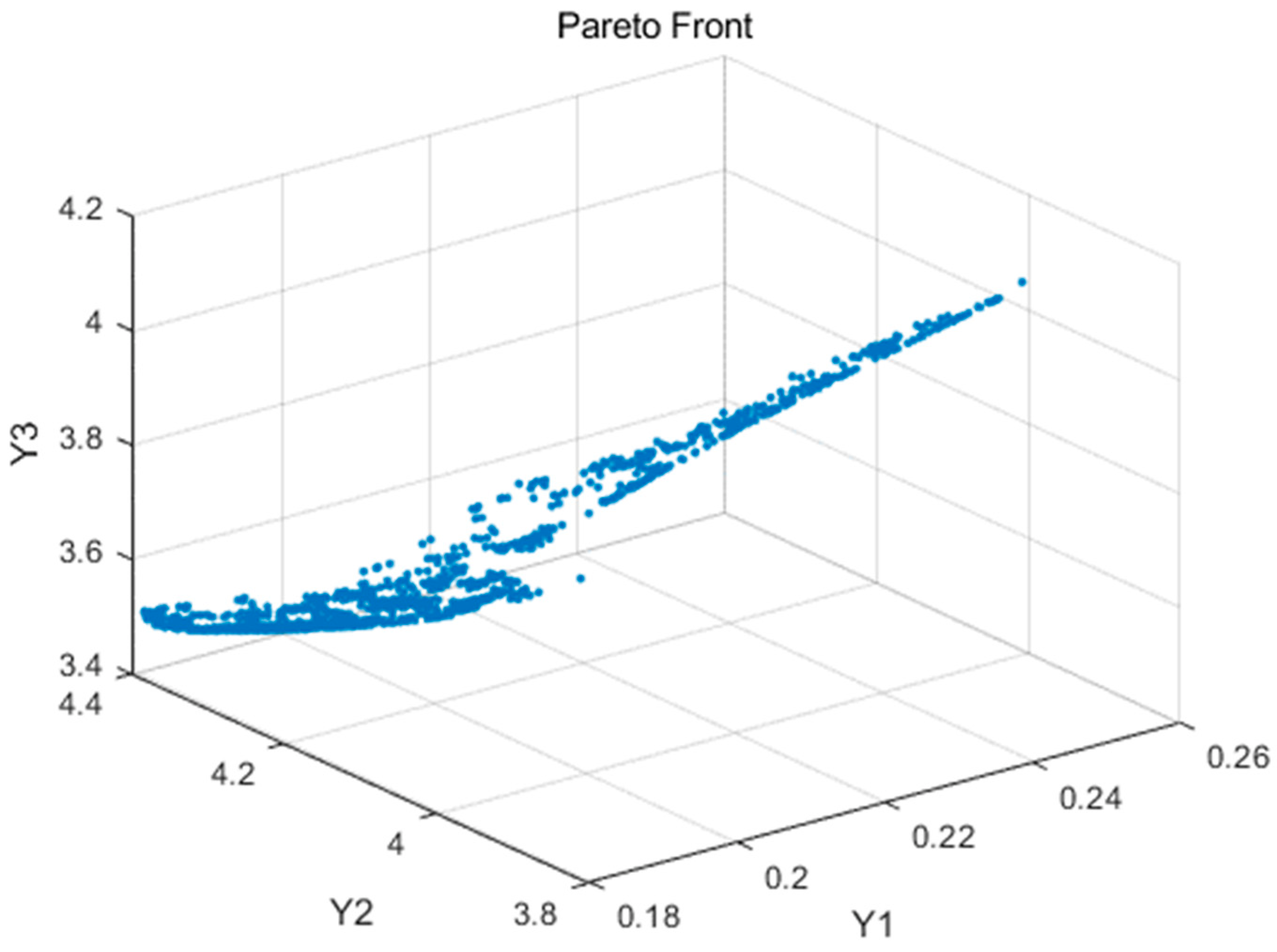
2.5. Multi-Objective Optimization Using Pareto Simulated Annealing Algorithm

The research suggests that in practical engineering multi-objective optimization problems, it is nearly impossible to find a single solution that optimizes all objectives. Traditional multi-objective optimization methods, such as the weighted sum method and goal programming, often require differentiation and are prone to becoming trapped in local optima. Simulated annealing (SA) is a randomized algorithm used for solving optimization problems.

The SA algorithm has a global optimal search capability, allowing it to escape local optima and adapt to complex optimization problems such as irregular and multi-peak issues. It requires relatively few parameters to be tuned, mainly the initial temperature and the cooling rate, making it easy to set up and use. The randomness of the algorithm allows for a broad exploration of the solution space in the initial phase, and as the temperature decreases, it refines the search, balancing the needs of exploration and exploitation. The algorithm is simple to implement and can be combined with other optimization algorithms to enhance performance. Based on the SA algorithm’s compatibility with other optimization methods, a simulated annealing algorithm combined with Pareto optimization can generate a Pareto optimal solution set, providing a selection of solutions that meet design requirements.

The core idea of solving the Pareto optimal solution set is to address the following multi-objective optimization problem [41]:

$$\min f\left(x\right)=f_1\left(x\right),f_2\left(x\right),\cdots ,f_n\left(x\right)$$

$$s.t.g\left(x\right)=0,h\left(x\right)\le 0,x\in X\subseteq R_n$$

(9)

If the variables x₁ ∈ R_n and x₂ ∈ R_n (where Rn represents the variable constraint set), and for all objective functions f_i(x₁) ≤ f_i(x₂) ( i = 1, 2,…, n), and there exists at least one objective function such that f_i(x₁) < f_i(x₂), then x₁ dominates x₂, denoted as x₁ > x₂. If there is no variable x and y in Rn such that y > x, then x is a non-dominated variable in Rn, and such a variable is the Pareto optimal solution in a multi-objective optimization problem. Pareto optimal solutions are often not only 1 optimal solution, but in the form of a set, so the key to multi-objective optimization is to find out as many optimal solutions as possible. The core process of multi-objective optimization of the Pareto SA algorithm is shown in Figure 4 [42].

Based on the Pareto optimal solution set, the SA algorithm is introduced to form the Pareto SA algorithm, which, according to the Metropolis criterion, makes the solution space accept the optimal solution while accepting the deterioration value with a certain probability in order to expand the global search capability, and the traditional single-objective optimization methods are often unable to deal with trade-offs among multiple objectives efficiently in the face of the complex multi-objective optimization problems. For this reason, this study combines the SA algorithm with the Pareto optimization approach, whose key lies in accepting the probability as the distance between the current solution and the new solution in the space. Its probability expression is as follows:

$$p\left(x\ge x^{\prime }\right)=\left\{\begin{array}{c}1f\left(x^{\prime }\right)<f\left(x\right)\\ \exp \left[{\displaystyle \frac{\sqrt{f^2\left(x^{\prime }\right)-f^2\left(x\right)}}{T}}\right]f\left(x^{\prime }\right)\ge f\left(x\right)\end{array}\right.$$

(10)

3. Results

In the formula, x is the current solution; x′ is the new solution; f(x) is the objective function value of the solution; and T is the temperature. Based on the above principles, Equations (6) to (8) were optimized by applying the SA algorithm using MATLAB software to obtain a Pareto solution. The initial temperature of the model is set to 100, the termination temperature is 1, the cooling rate is 0.9, and the maximum number of iterations is 5000. The Pareto optimal solution set of the multi-objective optimization problem of the quarry parameters is obtained using this method. In order to meet the actual engineering requirements and improve the economic benefits of the mine, it is recommended to appropriately reduce the width of the inter-columns and the thickness of the top slab left in place. Therefore, the Pareto optimal solution set is sorted in descending order according to the recovery rate, and the top 15 solutions are obtained, as shown in

Table 7. Optimization results of Pareto simulated annealing algorithm.

Serial Number	X1	X2	X3	Y1	Y2	Y3
1	15.003	10.000	11.901	0.251	3.916	4.132
2	15.000	10.005	12.129	0.247	3.916	4.114
3	15.000	10.020	12.112	0.247	3.919	4.111
4	15.000	10.049	12.078	0.247	3.923	4.105
5	15.002	10.053	12.078	0.247	3.925	4.104
6	15.003	10.043	12.100	0.247	3.923	4.105
7	15.000	10.001	12.178	0.247	3.917	4.112
8	15.000	10.000	12.180	0.247	3.917	4.112
9	15.000	10.000	12.191	0.247	3.917	4.112
10	15.000	10.073	12.093	0.246	3.928	4.097
11	15.000	10.070	12.100	0.246	3.927	4.097
12	15.007	10.031	12.220	0.245	3.925	4.101
13	15.000	10.058	12.233	0.244	3.928	4.091
14	15.000	10.087	12.195	0.244	3.932	4.086
15	15.002	10.102	12.184	0.244	3.935	4.082

. Figure 5 shows the Pareto frontier points of the target optimal solution set.

According to Table 7, Optimal Solution 1 (with a stope span of 15 m, pillar thickness of 10 m, and top pillar thickness of 11.9 m) represents the optimized structural parameters, and both the stope stress and displacement are within the controllable range of the limit mining dimensions, meeting engineering design requirements. However, despite these parameters being able to satisfy engineering design needs after optimization, some technical limitations may still arise during actual construction.

Firstly, the machinery required for construction must have sufficient capacity to handle specific rock types, mining depths, and the precision of stope structural parameters, as the efficiency and reliability of the equipment directly impact construction progress and safety. Secondly, different construction methods (such as explosive blasting or mechanical mining) have varying suitability and economic viability for different rock types, necessitating the selection of appropriate techniques based on specific strata and conditions.

Additionally, real-time monitoring technologies for stress, displacement, and groundwater levels need to be sufficiently advanced and accurate to provide timely feedback on the stability of the stope, allowing for the formulation of corresponding adjustment plans. Furthermore, the mechanical properties of the rock must be thoroughly studied to address complex geological conditions, especially when encountering brittle or plastic deformation in the strata, which may require more complex reinforcement and support techniques.

4. Discussion

In this study, the mechanical and displacement characteristics of the mine workings under different stope sizes were effectively verified through numerical simulation, and the relationships between them were established. A second-order nonlinear model was used to construct the relationships between the structural parameters and the mechanical responses, which clearly shows the complex interactive effects of the stope span, pillar span, and roof pillar thickness in terms of compressive stress and tensile stress. These interactive effects indicate that the mechanical response is not only influenced by a single parameter, but by the combined effects of multiple parameters.

Compared with traditional optimization methods, the Pareto SA algorithm can balance the weight of multiple parameters in multi-objective optimization problems and select the optimal mining structure parameters. The advantage of this method is that it can quickly find a set of non-dominated solutions, which can provide designers with diverse references in actual engineering. However, although the simulation results show strong relevance, the complexity and uncertainty of the model still need to be paid attention to. For example, in actual engineering, uncontrollable factors such as geological conditions and construction techniques may affect the accuracy of the model.

Future studies can further improve the reliability of the model by introducing more environmental factors or carrying out experimental verification. In addition, the combination of other advanced optimization algorithms such as genetic algorithms or deep learning models may also further optimize stope design schemes.

5. Conclusions

(1)

According to the K. Kgel strength formula, the safety coefficient of the pillar span should be greater than 1. The average span of the stope span is determined to be 15–20 m, and the width of the pillar span is 10–14 m. The thickness of the roof is calculated using the limit analysis method, and the thickness of the roof is calculated to be 10–14 m. Basic data support is provided for the subsequent optimization of the design.

(2)

The maximum tensile stress, maximum compressive stress, and maximum vertical displacement under different quarry parameters were obtained by numerical simulation through the means of the central composite test. The second-order response surface model between different parameters and each mechanical response was established, and the fitting R2 coefficients of each model were 0.98, 0.91, and 0.96 respectively, which indicated that the model fit was high and could be used for parameter optimization.

(3)

The SA algorithm based on the Pareto optimal solution set is applied to the multi-objective optimization problem of the response surface, and 15 non-inferior solutions are obtained for the structural parameters of the mining hall. According to the actual needs of the project and relevant principles, a stope span of 15.0 m, pillar span of 10.0 m, and thickness of the roof slab of 11.9 m are taken as the optimal structural parameters for mining.

References

1. Huang, M.; Wang, X.; Qiu Jixiang Gu Yazhou Cai, S.; Huang, M. Optimization of Mining Method for Stage Open-Stoping with Backfill of Inclined Medium-Thick Orebody. J. Min. Sci. Technol. 2024, 9, 483–492. [Google Scholar]
2. Sun, M.; Ren, F.; Ding, H. Optimization of Stope Structure Parameters Based on the Mined Orebody at the Meishan Iron Mine. Adv. Civ. Eng. 2021, 2021, 8052827. [Google Scholar] [CrossRef]
3. Sandanayake, D.S.S.; Topal, E.; Asad, M.W.A. A Heuristic Approach to Optimal Design of an Underground Mine Stope Layout. Appl. Soft Comput. 2015, 30, 595–603. [Google Scholar] [CrossRef]
4. Lan, M.; Liu, Z.X.; Li, X.B.; Liu, Q. Stope Parameters Optimization of Level Afterwards Back-Filling Approach with Medium-Deep Hole Caving. J. Cent. South Univ. (Sci. Technol.) 2018, 49, 933–939. [Google Scholar]
5. Zhou, X.; Zhao, X.; Qu, Q.; Shi, J. Stope Structural Parameters Design Towards Green and Deep Mining: A Review. Processes 2023, 11, 3125. [Google Scholar] [CrossRef]
6. Mawdesley, C.; Trueman, R.; Whiten, W.J. Extending the Mathews Stability Graph for Open–Stope Design. Min. Technol. 2001, 110, 27–39. [Google Scholar] [CrossRef]
7. Nan, S.; Gao, Q.; Liu, Z. Numerical Simulation of Fluid-Solid Coupling in Surrounding Rock and Parameter Optimization for Filling Mining. Procedia Eng. 2011, 26, 1639–1647. [Google Scholar]
8. Cui, X.; Yang, S.; Zhang, N.; Zhang, J. Optimization of Stope Structure Parameters by Combining Mathews Stability Chart Method with Numerical Analysis in Halazi Iron Mine. Heliyon 2024, 10, e26045. [Google Scholar] [CrossRef]
9. Hu, J.H.; Qin, Y.G.; Ren, Q.F.; Yang, D.J. Bearing Mechanism and Thickness Optimization of Ore Roof in Bauxite Stope. Trans. Nonferrous Met. Soc. China 2022, 32, 285–295. [Google Scholar]
10. Chen, S.; Wu, A.; Wang, Y.; Cheng, X. Multi-Objective Optimization of Stope Structure Parameters in Broken Rock Conditions Using Grey Relational Analysis. Arch. Min. Sci. 2018, 63, 269–282. [Google Scholar] [CrossRef]
11. Foroughi, S.; Hamidi, J.K.; Monjezi, M.; Nehring, M. The Integrated Optimization of Underground Stope Layout Designing and Production Scheduling Incorporating a Non-Dominated Sorting Genetic Algorithm (Nsga-Ii). Resour. Policy 2019, 63, 101408. [Google Scholar] [CrossRef]
12. Liu, X.; Liu, Z.X.; Liu, A.H.; Li, W. Chaotic Optimization of Structural Parameters in Gold Mining Field. J. Min. Saf. Eng. 2010, 27, 548–552. [Google Scholar]
13. Zhou, K.; Wang, X.; Gao, F. Stope Structural Parameters Optimization Based on Strength Reduction and Ann-Ga Model. J. Cent. South Univ. (Sci. Technol.) 2013, 44, 2848–2854. [Google Scholar]
14. Duh, J.D.; Brown, D.G. Knowledge-Informed Pareto Simulated Annealing for Multi-Objective Spatial Allocation. Comput. Environ. Urban Syst. 2007, 31, 253–281. [Google Scholar] [CrossRef]
15. Li, C.; Mei, X.; Zhang, J. Application of Supervised Random Forest Paradigms Based on Optimization and Post-Hoc Explanation in Underground Stope Stability Prediction. Appl. Soft Comput. 2024, 154, 111388. [Google Scholar] [CrossRef]
16. Matamoros ME, V.; Kumral, M. Heuristic Stope Layout Optimisation Accounting for Variable Stope Dimensions and Dilution Management. Int. J. Min. Miner. Eng. 2017, 8, 1–18. [Google Scholar] [CrossRef]
17. Nhleko, A.S.; Tholana, T.; Neingo, P.N. A Review of Underground Stope Boundary Optimization Algorithms. Resour. Policy 2018, 56, 59–69. [Google Scholar] [CrossRef]
18. Lee, K.S.; Geem, Z.W. A New Meta-Heuristic Algorithm for Continuous Engineering Optimization: Harmony Search Theory and Practice. Comput. Methods Appl. Mech. Eng. 2005, 194, 3902–3933. [Google Scholar] [CrossRef]
19. Rardin, R.L.; Uzsoy, R. Experimental Evaluation of Heuristic Optimization Algorithms: A Tutorial. J. Heuristics 2001, 7, 261–304. [Google Scholar] [CrossRef]
20. Hou, J.; Li, G.; Wang, H.; Hu, N. Genetic Algorithm to Simultaneously Optimise Stope Sequencing and Equipment Dispatching in Underground Short-Term Mine Planning under Time Uncertainty. Int. J. Min. Reclam. Environ. 2020, 34, 307–325. [Google Scholar] [CrossRef]
21. Zhai, S.; Gao, Q. Design and Optimization of Stope Parameters Based on Evolutionary Algorithm. J. Eng. Geol. 2015, 23, 699–705. [Google Scholar]
22. Martens, D.; De Backer, M.; Haesen, R.; Vanthienen, J.; Snoeck, M.; Baesens, B. Classification with Ant Colony Optimization. IEEE Trans. Evol. Comput. 2007, 11, 651–665. [Google Scholar] [CrossRef]
23. Leite, W.L.; Shen, Z.; Marcoulides, K.; Fisk, C.L.; Harring, J. Using Ant Colony Optimization for Sensitivity Analysis in Structural Equation Modeling. Struct. Equ. Model. A Multidiscip. J. 2022, 29, 47–56. [Google Scholar] [CrossRef]
24. Vasile, A.; Coropețchi, I.C.; Sorohan, Ș.; Picu, C.R.; Constantinescu, D.M. A Simulated Annealing Algorithm for Stiffness Optimization. Procedia Struct. Integr. 2022, 37, 857–864. [Google Scholar] [CrossRef]
25. Huri, D.; Mankovits, T. Surrogate Model-Based Parameter Tuning of Simulated Annealing Algorithm for the Shape Optimization of Automotive Rubber Bumpers. Appl. Sci. 2022, 12, 5451. [Google Scholar] [CrossRef]
26. Matamoros, M.E.V. A Novel Stope Layout Optimization Based on Robust Genetic Algorithms. Ph.D. Thesis, McGill University, Montreal, QC, Canada, 2018. [Google Scholar]
27. Saghatforoush, A.; Monjezi, M.; Shirani Faradonbeh, R.; Jahed Armaghani, D. Combination of Neural Network and Ant Colony Optimization Algorithms for Prediction and Optimization of Flyrock and Back-Break Induced by Blasting. Eng. Comput. 2016, 32, 255–266. [Google Scholar] [CrossRef]
28. Li, J.; He, Y.; Chang, L. Optimization of Stereo Parking Allocationbased on Improved Simulated Annealing Algorithm. J. Chongqing Univ. Technol. (Nat. Sci.) 2020, 34, 183–191. [Google Scholar]
29. Blanzeisky, W.; Cunningham, P. Using Pareto Simulated Annealing to Address Algorithmic Bias in Machine Learning. Knowl. Eng. Rev. 2022, 37, e5. [Google Scholar] [CrossRef]
30. Alkhamis, A.K.; Hosny, M. A Multi-Objective Simulated Annealing Local Search Algorithm in Memetic Censga: Application to Vaccination Allocation for Influenza. Sustainability 2023, 15, 15347. [Google Scholar] [CrossRef]
31. Sun, X.; Guo, S.; Guo, J.; Du, B.; Yang, Z.; Wang, K. A Pareto-Based Hybrid Genetic Simulated Annealing Algorithm for Multi-Objective Hybrid Production Line Balancing Problem Considering Disassembly and Assembly. Int. J. Prod. Res. 2024, 62, 4809–4830. [Google Scholar] [CrossRef]
32. Ma, H.T. Study on Method of Risk Classification and Instability Forecasting of Goaf; University of Science and Technology Beijing: Beijing, China, 2015. [Google Scholar]
33. Niu, X. Study on Roofs’ Stability of Cavities Under Open-Pit Mine; Changsha Institute of Mining Research Co., Ltd.: Changsha, China, 2013. [Google Scholar]
34. Wang, X.; Wu, X.; Sun, G. Numerical Simulation Analysis of Goafs Stability in Calcite Mine. Metal Mine 2015, 44, 24–27. [Google Scholar]
35. Zhang, W. Stability Analysis of Goaf and Optimization of Stope Parameters in a Calcite Mine. Mod. Minin 2020, 36, 80–83. [Google Scholar]
36. Allaix, D.L.; Carbone, V.I. An Improvement of the Response Surface Method. Struct. Saf. 2011, 33, 165–172. [Google Scholar] [CrossRef]
37. Shaibu, A.B.; Cho, B.R. Another View of Dual Response Surface Modeling and Optimization in Robust Parameter Design. Int. J. Adv. Manuf. Technol. 2009, 41, 631–641. [Google Scholar] [CrossRef]
38. Trinh, T.K.; Kang, L.S. Application of Response Surface Method as an Experimental Design to Optimize Coagulation Tests. Environ. Eng. Res. 2010, 15, 63–70. [Google Scholar] [CrossRef]
39. Xiao, X.W.; Xiao, D.; Lin, J.G.; Xiao, Y.F. Overview on Multi-Objective Optimization Problem Research. Appl. Res. Comput. 2011, 28, 805. [Google Scholar]
40. Mao, J.; Li, Q.; Xie, M.; Cao, J. Multi-Objective Optimization Software Development and Application. Chin. J. Eng. Des. 2015, 22, 262–268. [Google Scholar]
41. Wang, Z.; Rangaiah, G.P. Application and Analysis of Methods for Selecting an Optimal Solution from the Pareto-Optimal Front Obtained by Multiobjective Optimization. Ind. Eng. Chem. Res. 2017, 56, 560–574. [Google Scholar] [CrossRef]
42. Busetti, F. Simulated Annealing Overview. World Wide Web. Available online: https://r.search.yahoo.com/_ylt=AwrgxRIYzSpnLxMD4K9XNyoA;_ylu=Y29sbwNncTEEcG9zAzEEdnRpZAMEc2VjA3Ny/RV=2/RE=1732067864/RO=10/RU=http%3a%2f%2fwww.geocities.ws%2ffrancorbusetti%2fsaweb.pdf/RK=2/RS=R0RpaGrKiPpI6GnPOqrny1Dhiu8- (accessed on 12 April 2003).
Figure 1. Stope layout diagram.
Applsci 14 11597 g001
Figure 2. Finite element analysis model diagrams.
Applsci 14 11597 g002
Figure 3. Response surface of structural parameters and mechanical properties of different mining sites.
Applsci 14 11597 g003
Figure 4. Flow chart of Pareto simulated annealing algorithm.
Applsci 14 11597 g004
Figure 5. Pareto front points of the Pareto optimal solution set.
Applsci 14 11597 g005