Experimental and Numerical Investigations of Flat Approach Slab–Soil Interaction in Jointless Bridge

Abstract

In jointless bridges, a grade flat approach slab (GFAS) with the same elevation as the pavement can transfer the girder’s longitudinal deformation to the backfill. However, any cracks and settlement of the pavement usually occur at the end of the GFAS. To address this shortcoming, the buried flat approach slab (BFAS) horizontally embedded at a depth in the backfill was proposed. The complicated flat approach slab–soil interaction (FASSI) of the BFAS has not been systemically investigated. To address this gap, the influence of the FASSI on the mechanical performance of the approach slab and the backfill deformation was investigated in this research to understand the mechanism of the FASSI in absorbing one part of the girder’s longitudinal deformation and transferring the rest to the soil. Experimental tests on the FASSI with different embedded depths under longitudinal displacements were conducted. Numerical parametric analyses were carried out by considering the embedded depths and slab lengths as the parameters based on a finite element model verified using the test results. The results show that load–displacement curves of the FASSI comprise three stages: the elastic stage (approach slab’s displacement was absorbed by sand), the elastoplastic stage (sand deformation was observed), and the failure stage (overall shear failure of the sand was found). The longitudinal displacement transfer mode and vertical deformation distribution mode of the sand were affected by the embedded depth and slab length. With an increase in the embedded depth or a decrease in the slab length, the sand deformation decreases, which is beneficial for avoiding pavement crack risks and improving the pavement evenness. Finally, a simplified calculation formula that can be used to predict the load–displacement curves of the FASSI was proposed. This research provides the theoretical basis for the design and construction of the flat approach slab in jointless bridges.

1. Introduction

Expansion joints can be eliminated by exploiting the concept of a jointless bridge to essentially avoid noise while driving, reduced durability of the bridge, erosion of the substructure, and high maintenance costs resulting from damage to the expansion devices [1,2,3,4,5,6]. Due to its outstanding service performance, low life-cycle cost, and favorable economic and social benefits, jointless bridges have been widely applied [7,8,9,10,11]. For bridges with expansion joints, the longitudinal expansion and contraction deformation of the girder induced by temperature variations (u_t) can be absorbed by the gap at the expansion joint (Δu₀) installed between the girder end and the abutment backwall, as depicted in Figure 1. Therefore, no u_t will be transferred to the abutment backwall and approach slab. For jointless bridges, the approach slab is longitudinally connected to the girder to transfer the u_t to the soil of the connecting road [12,13,14,15,16,17], as depicted in Figure 2. The translation and rotation of the approach slabs due to the u_t can cause horizontal cracks and vertical settlement on the pavement of the connecting road at the junctions between the approach slab and the girder and at the end of the approach slab, as well as the settlement and cracking of the approach slab [18,19,20]. According to an investigation conducted by the Federal Highway Administration of the United States in 2004, the settlement and cracking of the approach slabs are two of the most prevalent diseases of jointless bridges in the United States, accounting for 46% and 28% of problems, respectively [21,22]. It can be pointed out that the approach slab must be considered in the design of jointless bridges [23,24,25].

The typical approach slab is a reinforced concrete (RC) solid slab. When the pavement of the connecting road is concrete pavement, a grade flat approach slab (GFAS) is commonly employed. The GFAS can be considered part of the pavement structure because its elevation is usually the same as the pavement of the connecting road [23]. In many states of the United States, the GFAS is adopted in the standard design drawing [26,27], of which the typical structure is shown in Figure 2a.

For a jointless bridge with a GFAS, u_t is mainly absorbed through soil deformation (Δu₂₃) within the range from x₂ to x₃ at the end of the GFAS, as shown in Figure 2a. Nevertheless, since the deformation is concentrated in one small area at the end of the GFAS, cracks and settlement of the pavement are prone to occur in that small area, and the corresponding maintenance expense increases [28,29]. To address this shortcoming, the buried flat approach slab (BFAS) was proposed and is now widely used in Europe, the United States, and Australia [14,20,30,31]. The BFAS is horizontally embedded at a depth (H), which can be calculated as the vertical distance from the pavement surface to the lower surface of the approach slab, of which the typical structure is shown in Figure 2b. The BFAS is particularly suitable for connecting roads with asphalt concrete pavement [2]. For a jointless bridge with a BFAS, cracks and settlement at the end of the approaching slab can be effectively reduced because u_t is mainly absorbed through soil deformation between x₁ and x₂ and between x₂ and x₃ above the BFAS, which can be denoted as Δu₁₂ and Δu₂₃, respectively, as shown in Figure 2b. GFASs and BFASs can be referred to as flat approach slabs (FASs) because the elevations at both ends are the same.

Under the influence of u_t, an interaction between the approach slab and the soil can be found, namely the approach slab–soil interaction (ASSI). The ASSI has been investigated by researchers through field monitoring, experimental tests, and theoretical analyses [31,32,33,34,35,36,37,38,39,40]. The service performance monitoring of a buried approach slab (BAS) indicated that a strain concentration is localized at the end of the approach slab and further extends obliquely upward from the end of the approach slab to the road surface [31,33]. Monitoring of the BAS in a jointless bridge revealed that when the temperature rises, the expansion of the girder pushes the BAS toward the connecting road, resulting in an increment in the compressive stress of the pavement; when the temperature drops, the contraction of the girder pulls the BAS away from the connecting road, resulting in a decrement in the stress of the pavement [34,35]. Experimental tests demonstrated that the longitudinal strains of the soil near the distal end of the approach slab and the pavement above the distal end of the approach slab are inversely proportional to H. With an increase in H, the risk of cracking on the pavement decreases [36]. The friction–displacement curves of a GFAS with different sliding materials installed between the bottom surface of the approach slab and the soil beneath it were simplified as a bilinear mathematical model by Tang et al. [33,41]. A simplified calculation model of a deck-extension jointless bridge with bilinear springs was established to analyze the influence of the GFAS on the mechanical performance of the deck-extension jointless bridge.

In summary, qualitative analyses on the influence of H on the strain distribution of embankment fill and the cracking of the pavement were conducted in existing studies. However, there is a lack of systematic analyses on the mechanism of the FAS in transferring and absorbing u_t by considering the mechanical performance of the approach slab and the deformation of the soil. Additionally, there is no quantitative analysis of the influence of H on the reduction of the settlement and cracking of the connecting road pavement. Moreover, the simplified calculation method on the flat approach slab–soil interaction (FASSI) is required.

To address this gap in the literature, investigations on the FASSI with different embedded depths and slab lengths were carried out. The rest of the paper is organized as follows: Section 2 presents the design and fabrication of the experimental test on the FASSI and discusses the test results, including the force–displacement curve, sand deformation, and earth pressure; Section 3 establishes a finite element model of the FASSI using software of PLAXIS 2D CE V20, the accuracy of which is verified by experimental data; Section 4 conducts a parametric analysis to investigate the influence mechanism of different embedded depths and slab lengths on the FASSI; Section 5 proposes a simplified calculation formula for the force–displacement curve of the FASSI, the accuracy of which is verified by the results of experimental tests and finite element models.

The research presented herein is of profound significance for the design and construction of BFASs in jointless bridges. Specifically, by delving deeply into the understanding of the mechanism of FASs in transferring and absorbing longitudinal displacement, especially by conducting quantitative analyses on the longitudinal displacement transfer mode (LDM) and vertical deformation distribution mode (VDM) of the sand, optimized designs that minimize the potential risk of pavement cracking can be obtained. These include the arrangement positions of geogrids in the sand and elastic materials at the end of the approach slab. Moreover, the simplified calculation formula for predicting the force–displacement curve of the FASSI can calculate spring stiffness for numerical models of jointless bridges, presenting a novel method for the design of FASs in jointless bridges.

2. Experimental Test

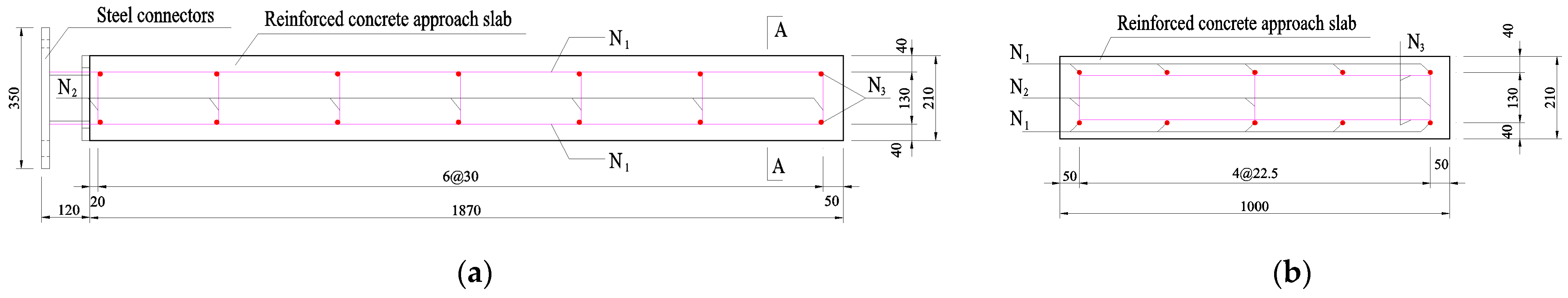
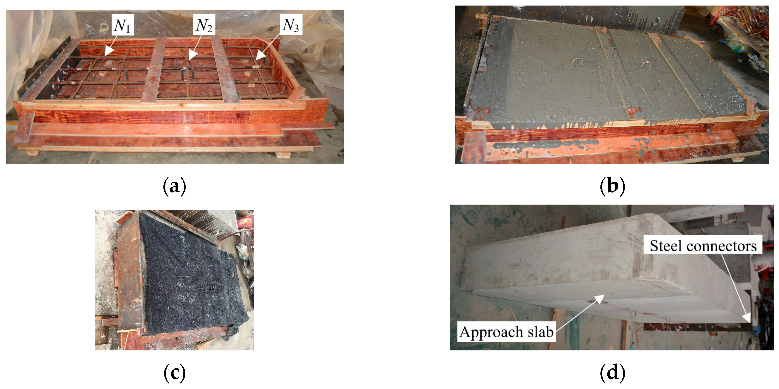
2.1. Specimen Design and Fabrication

A FAS specimen with a length × width × depth of 1.87 m × 1 m × 0.25 m was designed. Concrete of strength grade C30 was employed. The HRB400 ribbed rebars with a 10 mm diameter were arranged in the slab (N₁, N₂, and N₃) to reach a reinforcement ratio of 6%, as shown in Figure 3. The fabrication processes of the FAS specimen consisted of the installation of the formwork and rebar cages (Figure 4a), the concrete casting (Figure 4b), and concrete curing at normal atmospheric temperature (Figure 4c) followed by formwork removal after 28 days to obtain the FAS specimen (Figure 4d). The 28-day cube strength (f_cu) and elastic modulus (E_c) of the concrete measured from compressive tests on cubic and prism specimens were found to be 20.23 MPa and 29.5 GPa, respectively. The yield strength (f_y) and elastic modulus (E_r) of the rebar obtained from tensile tests were found to be 405 MPa and 195 GPa, respectively.

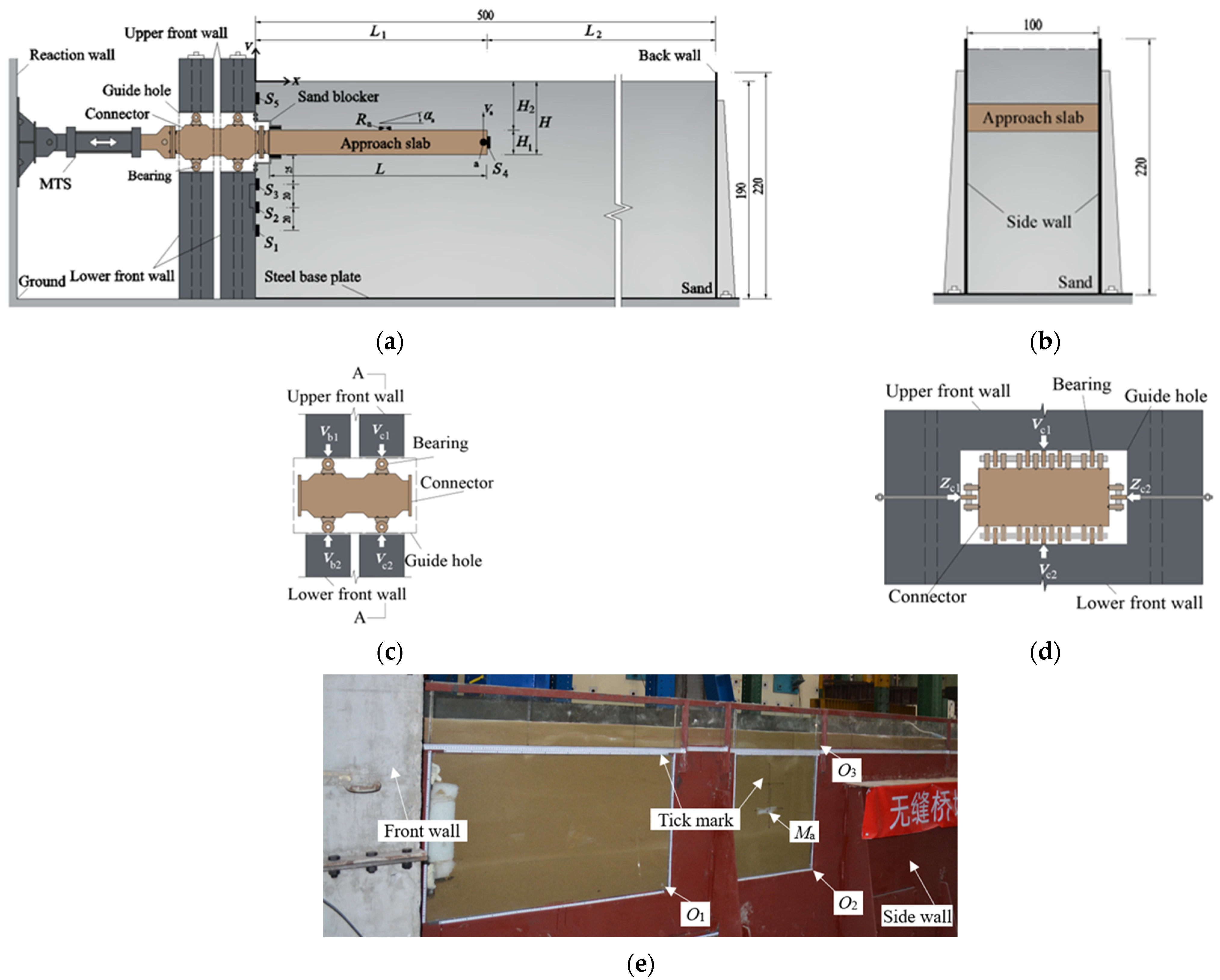
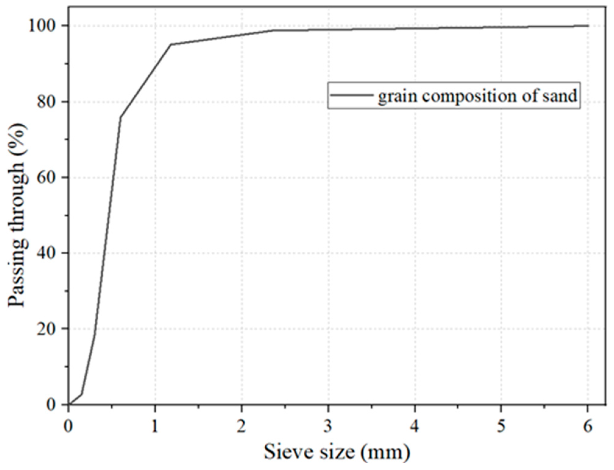
2.2. Soil Container Design and Fabrication

Rigid containers have previously been used by some researchers to investigate the structure–soil interaction [24,42,43,44]. A rigid cuboid container with a length × width × depth of 5 m × 1 m × 2.2 m was designed and fabricated, as shown in Figure 5a,b. The container consists of a concrete front wall, two steel side walls, a steel back wall, and a steel base plate, which are fixed on the ground by anchors. The influence of the boundary of the container on the slip surface formed when the sand behind the distal end of the FAS reaches the limit equilibrium state due to the movement of the FAS can be neglected if the length (L₂) from the distal end of the FAS to the front surface of the back wall (as shown in Figure 5a) is larger than the theoretical length (L_2.th) calculated by using Formula (1). Based on the friction angle (φ_s = 35°) of the sand, the maximum H (63 cm) in the test conditions, and the horizontal angle (θ = 45 + φ_s/2) [45] of the slip surface of the sand at x₃ in Figure 2b, L_2.th can be calculated as 121 cm. Considering uncertainties, L₂ was chosen as 300 cm, as shown in Figure 5a.

L_2.th = H·tan (45 + φ_s/2) = 121 cm

(1)

Two concrete walls with guide holes were longitudinally arranged to serve as the front wall of the container. The connector passed through the guide holes longitudinally connects the electro-hydraulic servo loading system (MTS) and the proximal end of the FAS specimen to transfer the longitudinal displacement (u_t) of the MTS to the FAS specimen. A fixed constraint at the proximal end of the FAS specimen can be obtained by setting two sets of bearings installed at the top and bottom surfaces of the connector, which restrict the vertical movements of the connector at points V_a1, V_a2, V_b1, and V_b2 and the rotation of the connector around the lateral axis, as shown in Figure 5c. Two sets of bearings installed at the left and right surfaces of the connector restrict the lateral movements of the connector at points Z_c1 and Z_c2, as shown in Figure 5d. The influence of friction on the connector can be eliminated through bearings.

To prevent sand from flowing into the guide holes during the loading process, two sand blockers were installed at the proximal end of the FAS specimen. Butter was applied between the FAS specimen and sand blockers to eliminate the influence of friction. Three rectangular tempered glass observation windows, O₁ to O₃, were installed on one side wall, as shown in Figure 5e. Longitudinal and vertical tick marks were arranged on the observation windows, which can be used to record the translation and rotation of the FAS specimen, as well as the deformation of the sand surface, and the development and formation process of the slip surface of the sand.

Sand from the Minjiang River in Fujian Province was selected, which was characterized by a 1.51 g/cm³ density (ρ). The particle grading curve is shown in Figure 6. Particle size distribution tests on three groups of sand samples at different depths in the container were carried out to obtain the measured non-uniformity coefficient (C_u) and the curvature coefficient (C_c) of the sand, which were found to be 2.32 and 1.47, respectively. Direct shear tests on the sand samples under different vertical pressures were conducted. The calibration coefficient of the direct shear apparatus dynamometer (C) was found to be 1.82 kPa/0.01 mm, and the measured average internal friction angle of the sand (φ_s) was 35.0°. The moisture content measured by the drying method was found to be 4.6% (mass fraction). According to the “Code for Investigation of Geotechnical Engineering” [46], the test sand was the same dense sandy soil as that in many real applications with a 68% relative density. The sand was gradually filled and compacted layer by layer, with each layer being approximately 25 cm in height, until the total height reached 1.9 m.

2.3. Test Cases and Set-Up

Four embedded depths (H) were set as the test parameters. For each H, two displacement directions were considered, which are push (away from the front wall) and pull (toward the front wall). Therefore, eight test cases were obtained, the detailed information on which is listed in

Table 1. Characteristic points in F-u curves.

H (cm)	Loading Direction	Test Cases	a		b		c		k (kN/mm)	l (kN/mm)
			ua (mm)	Fa (kN)	ub (mm)	Fb (kN)	uc (mm)	Fu (kN)
0	Push	H0-Push	0.52	4.81	1.52	5	50	5.85	9.25	0.02
21		H21-Push	0.61	6.36	3.38	7.2	50	9.51	10.43	0.05
31.5		H31.5-Push	0.75	8.43	6.42	15.3	50	17.71	11.24	0.06
63		H63-Push	1.42	26.41	8.74	35.5	50	35.62	18.60	0.00
0	Pull	H0-Pull	−0.45	−2.73	−2.45	−5.1	−50	−6.75	6.07	0.03
21		H21-Pull	−0.56	−3.84	−2.58	−7	−50	−7.82	6.86	0.02
31.5		H31.5-Pull	−1.21	−8.74	−3.66	−10.3	−50	−13.35	7.22	0.07
63		H63-Pull	−1.41	−18.12	−5.27	−18.6	−50	−31.7	12.85	0.29

and illustrated in Figure 5a. In the table, the first part of the label (H0, H21, H31.5, or H63) indicates the embedded depth of the FAS specimen calculated from the sand surface to its lower surface and the second part of the label (Push or Pull) indicates the displacement direction. For example, H63-Push represents the test case of a FAS specimen with a 63 cm H subjected to a push u_t.

The test set-up consists of a rigid soil container, sand, FAS specimen, connector, and MTS, as illustrated in Figure 5a. The installation steps of the test set-up were as follows: (1) assemble the rigid soil container; (2) fill and compact the sand under the FAS specimen; (3) erect the FAS specimen; (4) fill and compact the sand above the FAS specimen; and (5) connect the FAS specimen, connector, and MTS hydraulic actuator. A horizontal displacement (u_t) was applied to the proximal end of the FAS specimen by an MTS hydraulic actuator using a displacement-control method with a peak u_t of ±50 mm. The load rate was 1 mm/s [43].

2.4. Instrument Setup

Different types of measurement instruments were employed, as shown in Figure 5a. The load–displacement (F-u) curves can be obtained from the MTS system. The end of the FAS specimen that is far from the MTS is defined as the distal end and the end of the FAS specimen close to the MTS is defined as the proximal end.

A displacement observation point (a) was set at the distal end of the FAS specimen, as shown in Figure 5a. The vertical displacement of point a (v_a) (upward is defined as the positive value) can be measured through observation window O₂. The horizontal angle (θ) of the sand slip surface can be measured through observation windows O₁ and O₂. The deformation position (x) (away from the MTS is defined as the positive value) and the vertical deformation (v_s) (upward is defined as the positive value) of the sand surface can be measured through observation window O₃.

An inclinometer (R_a) was installed at the mid-length point of the specimen’s top surface to measure the rotation angle of the FAS specimen (α_a) (counterclockwise rotation is defined as the positive α_a). Five earth pressure cells (S₁ to S₅) were arranged. The earth pressures are negative values. S₁ to S₃ were arranged from low to high on the back surface of the lower part of the front wall each with a height interval of 20 cm. S₃ was 25 cm lower than the bottom surface of the FAS specimen. S₄ was installed at the mid-thickness point of the distal end surface of the FAS specimen. S₅ was arranged at the mid-height point of the back surface of the upper part of the front wall. The values of the MTS system, inclinometer, and earth pressure cells were set to zero before the commencement of the test.

2.5. Experimental Results

2.5.1. Specimen Movement

Under push u_t, the FAS specimen slightly rotates counterclockwise with a maximum α_a of +0.04°, and its distal end moves upward with a maximum v_a of +1.8 mm. Under pull u_t, the FAS specimen slightly rotates clockwise with a maximum α_a of −0.02°, and the distal end moves downward with a maximum v_a of −0.86 mm. The rotation and translation of the FAS under push u_t are slightly larger than those under pull u_t. This is because the amount of sand above the FAS specimen is less than that below it, and there is no constraint on the top surface of the sand. The rotation and translation are relatively small in real applications. It can be proposed that the FAS mainly horizontally moves along the displacement direction.

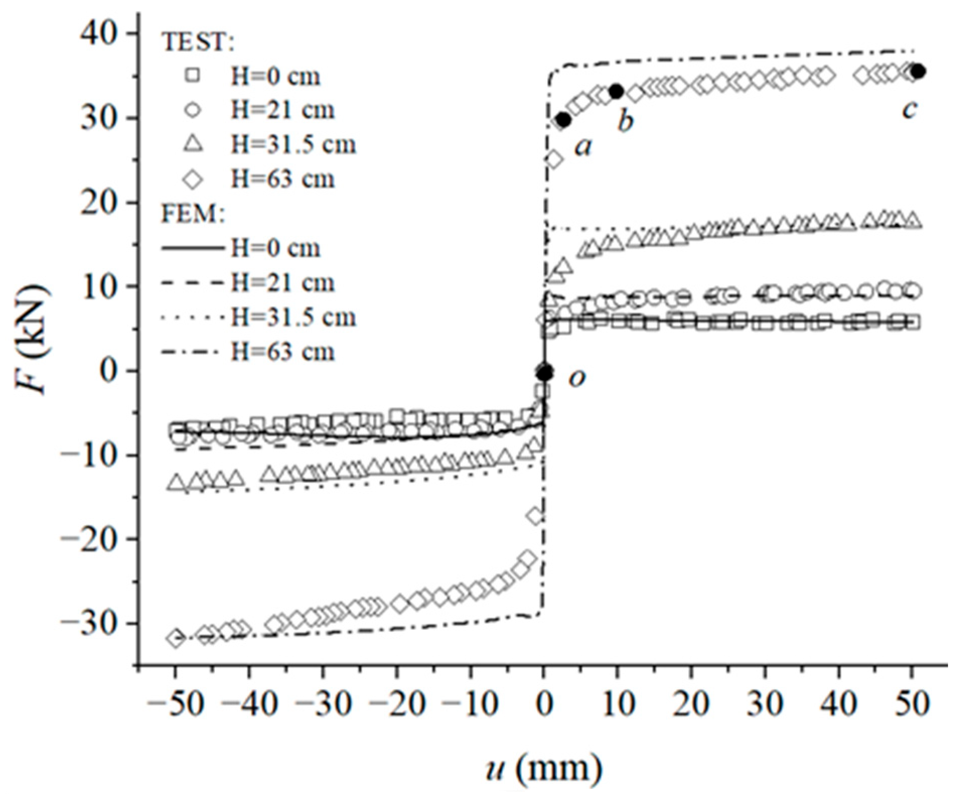
2.5.2. Load–Displacement Curve

The load–displacement (F-u) curves of different test cases are illustrated in Figure 7. The hollow symbols denote the F-u curves obtained from experimental tests. Taking the F-u curve of H63-Push as an example, the characteristic points (o, a, b, and c) of the curve are marked with solid circles. The u corresponding to each characteristic point are u_a, u_b, and u_c, respectively, and the corresponding F are F_a, F_b, and F_u, respectively. With an increase in u, the F-u curves under push or pull u_t exhibit similar characteristics, which can be divided into three stages.

• Elastic stage oa: when u is less than u_a, F and u exhibit a linear relationship. The sand is in an elastic state, and the stiffness of the curve is k.
• Elastoplastic stage ab: when u is between u_a and u_b, the internal stress of the sand is redistributed, and some soil particles slip relatively. The sand enters a plastic state, and the k gradually decreases.
• Failure stage bc: when u is larger than u_b, the sand in the plastic state gradually forms a slip surface. With a rapid increase in u, F increases slightly. The stiffness of the curve decreases to l. The value of F_u at point c is the ultimate load.

Figure 7. F-u curves obtained from tests and finite element models.

Figure 7. F-u curves obtained from tests and finite element models.

The characteristic points of the F-u curves in different test cases and corresponding k and l are listed in Table 1. It can be found that with an increase in H, F_a, F_b, F_u, and k increase, while l is very small. This is because, in the elastic stage, the movement of the FAS specimen is affected by the friction between the top and bottom surfaces of the FAS specimen and the sand above and below it, as well as the earth pressure at the distal end of the FAS specimen. With an increase in H, the mass of the sand above the FAS specimen increases, resulting in an increment in the friction force between the FAS specimen and the sand, and the earth pressure at the distal end of the FAS specimen. In the failure stage, after the slip surface of the sand is formed, F, the friction force, and the earth pressure on the FAS specimen reach a state of mechanical equilibrium. Therefore, F largely stops increasing and l is nearly zero.

Under push u_t, the increments in H changing from H0-Push to H31.5-Push and from H31.5-Push to H63-Push are both 31.5 cm and the corresponding F_u values increase by 11.9 kN and 17.9 kN, respectively. Under pull u_t, the increments in H changing from H0-Push to H31.5-Push and from H31.5-Push to H63-Push are both 31.5 cm and the corresponding F_u values increase by 6.6 kN and 18.4 kN, respectively. It can be concluded that with an increase in H, the increment rate of F_u increases. This is because the slip surface formed in the failure stage develops obliquely upward from the distal end of the FAS specimen. The larger the H, the wider the range of sand affected by the distal end of the FAS specimen.

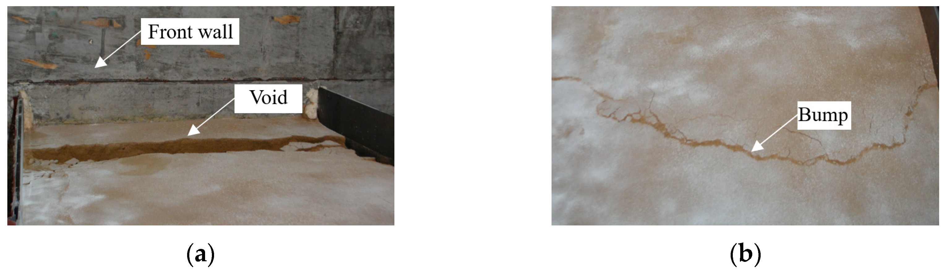
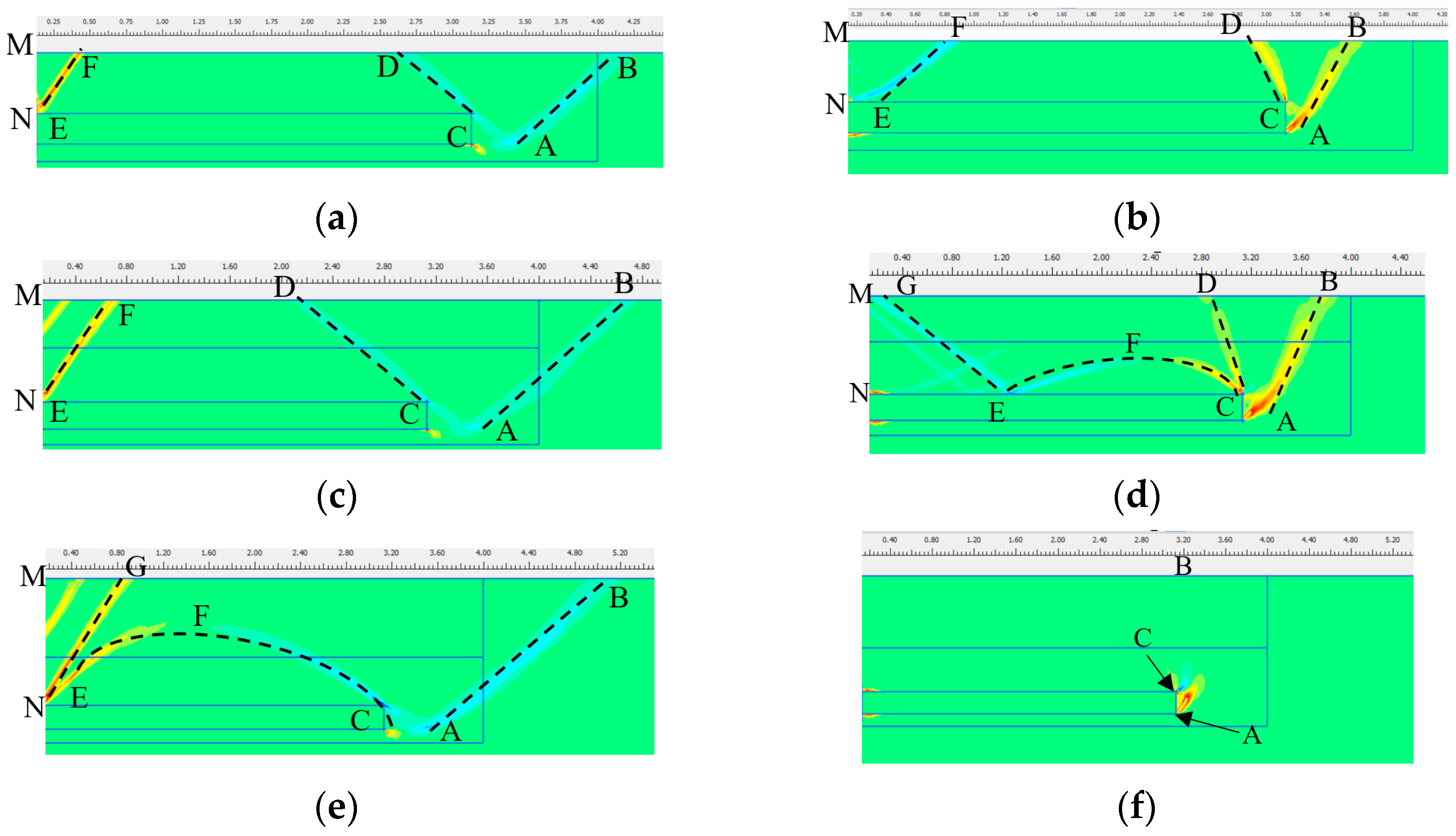
2.5.3. Sand Deformation

To ensure the accuracy of the sand surface deformation measurements, the sand surface was leveled before applying displacement. Under push u_t, a void can be found at the sand surface near the proximal end of the FAS specimen, while a bump can be found at the sand surface near the distal end. The sand surface deformation of H63-Push under a +50 mm u_t is illustrated in Figure 8. Under pull u_t, a bump can be found at the sand surface near the proximal end of the FAS specimen, while a void can be found at the sand surface near the distal end. The sand surface deformation of H63-Push under a −50 mm u_t is shown in Figure 9.

The sand surface deformations of different test cases observed through observation windows O₁ to O₃ are compared in Figure 10.

From the F-u curves and the sand surface deformation diagrams under different u_t, it is found that the sand surface deformations under push and pull u_t exhibit similar characteristics, which can be divided into three stages:

• Elastic stage

When u is less than u_a, the FAS specimens under push and pull u_t demonstrate coordinated deformation characteristics with the sand. The elastic deformation of the sand can efficiently absorb u. No obvious crack or deformation can be observed on the sand surface.

• Elastoplastic stage

When u is between u_a and u_b, certain areas of the sand (as indicated by the dotted line in Figure 10) gradually transform from elastic deformation to plastic deformation. The sand in the area demarcated by the dotted lines moves as depicted by the arrows in Figure 10. Remarkable differences in the deformation modes of the sand under push and pull u_t can be observed.

Under push u_t, at the dashed line AB, the sand moves upwards to the point x_2b on the sand surface along the horizontal angle θ_2b from A to B; at the dashed line CD, the sand moves upwards to the point x_2a on the sand surface along the horizontal angle θ_2a from C to D; and at the dashed line EF, the sand moves downwards from the point x_1b on the sand surface along the horizontal angle θ_1b from F to E. Consequently, a bump with a width of w₂ and a height of v_s2 can be found on the sand surface from x_2a to x_2b near the distal end of the FAS specimen and a void with a width of w₁ and a depth of v_s1 can be found on the sand surface from x_1a to x_1b near the proximal end of the FAS specimen.

Under pull u_t, at the dashed line AB, the sand moves downwards from the point x_2b on the sand surface along the horizontal angle θ_2b from B to A; at the dashed line CD, the sand moves downwards from the point x_2a on the sand surface along the horizontal angle of θ_2a from D to C; and at the dashed line EF, the sand moves upwards to the point x_1b on the sand surface along the horizontal angle of θ_1b from E to F. Consequently, a bump with a width of w₁ and a height of v_s1 can be found on the sand surface from x_1a to x_1b near the proximal end of the FAS specimen and a void with a width of w₂ and a depth of v_s2 can be found on the sand surface from x_2a to x_2b near the distal end of the FAS specimen;

The reason for these observed deformations is that under push u_t, the sand zone EFG at the proximal end of the FAS specimen moves far away from the front wall, resulting in a deformation trend of sliding downwards. The sand surface subsides and forms a void. The sand zone ABD at the distal end of the FAS specimen is compressed by the FAS specimen, resulting in a deformation trend of sliding upwards. The sand surface uplifts and forms a bump. Under pull u_t, the sand zone EFG at the proximal end of the FAS specimen moves towards the front wall, resulting in a deformation trend of sliding upwards. The sand surface uplifts and forms a bump. The FAS specimen moves far away from the sand zone ABD at its distal end, resulting in a deformation trend of sliding downwards. The sand surface subsides and forms a void. The sand around the FAS specimen has formed a plastic zone. With an increase in u, the sand deformation around the FAS specimen is gradually transferred to the sand surface. Because one part of u can be absorbed by sand deformation, the deformation of the sand surface increases slowly.

• Failure stage

When u is larger than u_b, with an increase in u, the deformations of the sand zones EFG and ABD at the distal and proximal ends of the FAS specimen increase rapidly under push and pull u_t. Shear failure can be found in the sand around the FAS specimens, and the plastic region inside the sand expands continuously to form a plastic zone extending from the FAS specimen to the sand surface along a certain horizontal angle θ. With the development of the plastic zone, a continuous slip surface is finally formed, such as the zones shown by the dotted line in Figure 10.

Under push u_t, at the distal end of the FAS specimen, a passive deformation zone ABD in a compressive state is formed by the slip surfaces AB and CD and the sand surface. At the proximal end of the FAS specimen, an active deformation zone EFG in a tensile state is formed by the slip surface EF, the front wall EG, and the sand surface.

Under pull u_t, at the distal end of the FAS specimen, an active deformation zone ABD in a tensile state is formed by the slip surfaces AB and CD and the sand surface. At the proximal end of the FAS specimen, a passive deformation zone EFG in a compressive state is formed by the slip surface EF, the front wall EG, and the sand surface.

The parameters of the sand deformation and slip surface of different test cases are summarized in

Table 2. Parameters of sand surface deformation.

Parameters	x1a	x1b	w1	vs1	x2a	x2b	w2	vs2	θ1b	θ2a	θ2b
Units	m			mm	m			mm	°
H21-Push	/	/	/	/	2.05	2.47	0.42	40	/	/	36
H31.5-Push	0.13	0.19	0.06	−55	1.91	2.74	0.83	38	71	53	39
H63-Push	0.12	0.39	0.27	−42	1.67	3.04	1.36	36	70	49	38
H21-Pull	/	/	/	/	2.10	2.23	0.13	−72	/	/	74
H31.5-Pull	0.00	0.32	0.32	18	1.94	2.19	0.24	−38	35	78	76
H63-Pull	0.00	0.82	0.82	15	1.90	2.26	0.35	−35	32	65	77

. It can be found that with an increase in H, w₂ increases, while v_s2 decreases. The reason for this is that the sand deformation zone is a wedge-shaped zone that gradually enlarges from the bottom to the top. The larger the H, the larger the area of the wedge-shaped zone, and the more u that can be absorbed. With an increase in H, the pavement deformation decreases, and the risk of pavement settlement and cracking can be reduced, which is similar to the conclusions in [21,34,47].

Compared with the influence of H on θ_2a and θ_2b, as shown in Figure 10, it can be found that θ_2a decreases by 4° and θ_2b decreases by 1° when H increases from 31.5 cm to 63 cm under push u_t. θ_2a decreases by 13°, and θ_2b decreases by 1° when H increases from 31.5 cm to 63 cm under pull u_t. Therefore, it can be concluded that with an increase in H, θ_2a gradually decreases, while θ_2b remains nearly the same. θ_2a is relatively larger than θ_2b because, when H is the same, compared with the slip surface AB, the shear deformation of the sand at the slip surface CD is restricted by the frictional effect between the upper surface of the FAS specimen and the sand above it. When H is small, the sand above the FAS specimen is thin, and the friction on the FAS specimen is large, resulting in θ_2a being relatively larger than θ_2b. With an increase in H, the influence of friction on the FAS specimen gradually decreases, resulting in a smaller θ_2a.

The variations in θ_2b and θ_1b with H are both less than 3°, as shown in Figure 10, because they are not affected by the friction between the FAS specimen and the sand. The measured θ_2b and θ_1b were compared with Rankine’s theoretical earth pressure. It can be found that θ_2b in the passive state of approximately 37.6° under push u_t and θ_1b in the passive state of approximately 33.5° under pull u_t are 10.1° and 6° larger than the horizontal angle θ_r.p = 45° − φ_s/2 = 27.5° of Rankine’s passive earth pressure, respectively. θ_2b in the active state of approximately 75.6° under pull u_t and θ_1b in the active state of approximately 60.5° under push u_t are 13.1° and 8° larger than the horizontal angle θ_r.a = 45° + φ_s/2 = 62.5° of Rankine’s active earth pressure, respectively. The differences may be related to the existence of matric suction in the sand. Matric suction enhances the binding force between soil particles, which is equivalent to increasing φ_s [48,49]. In addition, factors such as the particle gradation and compactness of the sand may also affect the horizontal angle of the slip surface.

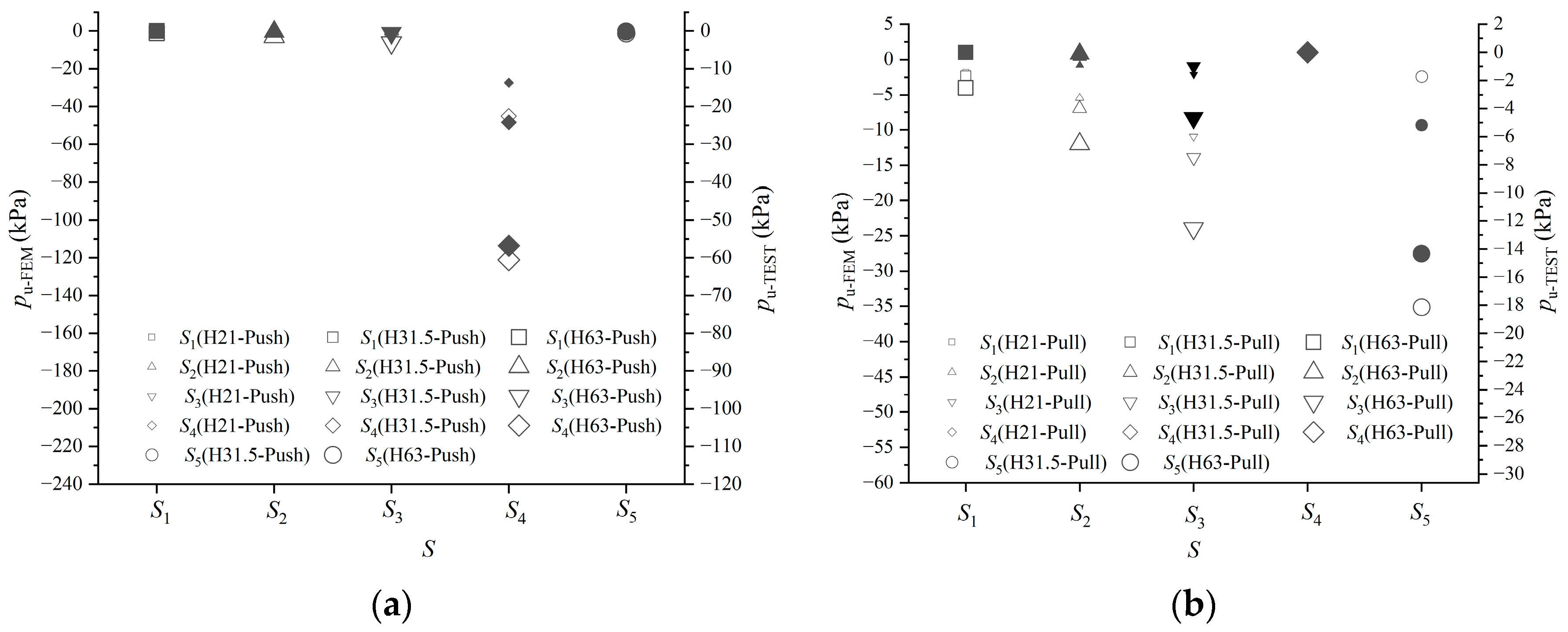
2.5.4. Earth Pressure

To eliminate the influence of the initial value difference on the measured data, the earth pressure gauge was set to zero after filling the sand and completing the installation of the specimen. The earth pressure–displacement (p-u) curves of different test cases are illustrated in Figure 11. The p-u curves of the test cases under push u_t are significantly different from those under pull u_t.

Under push u_t, with an increase in u, the p of S₄ (the distal end of the FAS specimen) first rapidly increases, and then slightly increases, as shown in Figure 11a. With an increase in H, p increases up to a maximum value of 56.78 kPa. This is because, with an increase in u, the sand at the distal end of the FAS specimen gradually approaches the limit bearing capacity state, and a slip surface is formed near the distal end of the FAS specimen. When a slip surface is formed, the peak resistance of the sand to the FAS specimen can be obtained, and the increment in p is significantly reduced. With an increase in H, the effective vertical stress in the sand increases, resulting in the increment of the earth pressure at the distal end of the FAS specimen. With an increase in u, the FAS specimen gradually moves away from the front wall. The p of S₁ to S₃ (lower part of the front wall) and S₅ (upper part of the front wall) are nearly zero. This is because, when the FAS specimen gradually moves away from the front wall, the earth pressures of S₁ to S₃ and S₅ decrease from the static earth pressure to the active earth pressure. The sand in some positions may even separate from the front wall to form voids.

Under pull u_t, with an increase in u, the p of S₅ (upper part of the front wall) rapidly increases firstly, and then slightly increases, as shown in Figure 11b. This is because the earth pressure of S₅ increases from the static earth pressure to the passive earth pressure. The maximum p is 14.64 kPa when H is 63 cm. With an increase in H and u, the p of S₁ to S₃ (lower part of the front wall) increased. The reason for this is that the mass of the FAS specimen and the sand above it produce additional stress on the sand below it [49]. The magnitude of the stress is proportional to the mass of the FAS specimen and the sand above it, and inversely proportional to the distance from the mid-length point of the lower surface of the FAS specimen. Therefore, with an increase in u, the FAS specimen moves closer to the front wall. From S₁ to S₃, the corresponding distance to the mid-length point of the lower surface of the FAS specimen decreases, resulting in a larger additional stress and an increment in p. With an increase in H, the mass of the FAS specimen and the sand above it increase, resulting in a larger additional stress and an increment in p. In addition, the maximum p decreases from S₁ to S₃. This is because, from S₁ to S₃, the distance to the mid-length point of the lower surface of the FAS specimen gradually increases, and the additional stress correspondingly decreases. The maximum p can be found at S₃ and is 4.86 kPa.

In summary, the p values of S₁ to S₃ (lower part of the front wall) are smaller than that of S₅ (upper part of the front wall). The p of S₄ (the distal end of the FAS specimen) is very small. This is because the earth pressure of S₄ decreases from the static earth pressure to the active earth pressure. The sand in some positions may even separate from the front wall to form some voids.

3. Finite Element Simulation and Verification

3.1. Finite Element Model Simulation

3.1.1. Model Introduction

During the test, the lateral deformations of the FAS specimen and sand were significantly less than the longitudinal and vertical deformations. Consequently, the test model can be considered as a plane strain problem [50,51,52,53]. The finite element model (FEM) of FASSI was established using the two-dimensional geotechnical finite element software Plaxis2D, as illustrated in Figure 12. The average element size of the FEM was 5 × 10⁻³ m. The element sizes around the FAS specimen and the front wall were refined to improve the calculation accuracy.

3.1.2. Material Properties

The material constitutive models of the FEM were determined through the tests on the material characteristics presented in Section 2.1. An elastic material constitutive model was chosen for the concrete with a 29.5 GPa E_c, 24 kN/m³ unit weight of concrete (γ_c), and 0.25 Poisson’s ratio of concrete (υ_c). A Mohr–Coulomb constitutive model was used for the sand with a 19 MPa elastic modulus of sand (E_s), 19 kN/m³ unit weight of sand (γ_s), 35° internal friction angle of sand (φ_s), 11.67°dilation angle of sand (ψ_s), which is equal to 2φ_s/3, 0.1 cohesion of sand (c_s), and 0.3 Poisson’s ratio of sand (υ_s) [54].

3.1.3. Boundary Conditions

To simulate the restraining effect of the soil container on the sand, the translational degrees of freedom in the X and Y directions of the left nodes of the front wall, the X direction of the right nodes of the sand, and the Y direction of the bottom nodes of the sand were restrained. To simulate the fixed-end constraint at the proximal end of the FAS specimen and the load imposed by the MTS, the rotational and translational degrees of freedom in the Y direction were restrained at the loading point. u_t was applied in the X direction at the loading point.

The FAS specimen–sand interaction was simulated using the interface element in Plaxis2D [55]. The interface element, which has the same Mohr–Coulomb constitutive model as the sand, was connected to the nearby approach slab and soil elements by five sets of nodes. The interface element was characterized by the strength reduction coefficient R_inter, which can establish a correlation between soil strength (φ_s, c_s) and interface strength (φ_inter, c_inter) by Formula (2) [56], where φ_inter and c_inter represent the internal friction angle and cohesion of the interface element, respectively.

tan φ_inter = R_inter · tanφ_s, c_inter = R_inter · c_s

(2)

Two interfaces were considered in the FEM, namely, the interface between concrete and sand with a 0.91 R_inter [55] and the interface between the sand blocker and the FAS specimen with a very small R_inter of 0.1 to simulate the lubricating effect of the butter. Furthermore, the gap of the interface open or closing is configured to simulate the real behavior of sand. A gap is created between the sand and the FAS when the interface is under tension, and the gap is closed by filling the sand when the interface is not under tension.

The loading procedure in the FEM can be divided into two steps. The initial stress equilibrium is the first step. The K₀ technique can be used to directly generate the initial effective stress because of the horizontal sand surface [55]. The equation K₀ = 1 − sinφ_s is the default approach used in Plaxis2D to calculate K₀ of typically consolidated soil [55]. Applying u_t at the loading point of the FAS specimen is the second step.

3.2. Finite Element Model Verification

3.2.1. Specimen Movement

Under push u_t, the maximum α_a and v_a are +0.01°and +0.38 mm, respectively. Thus, it can be concluded that the FAS specimen undergoes a slight counterclockwise rotation and upward movement at the distal end. Under pull u_t, the maximum α_a and v_a are −0.01° and −0.01 mm, respectively. Thus, it can be concluded that the FAS specimen undergoes a slight clockwise rotation and downward movement at the distal end. The specimen movement obtained from the FEM is in accordance with that observed in the test, as discussed in Section 2.5.1. This demonstrates that the FEM can reflect the actual movement trend of the FAS specimen.

3.2.2. Load–Displacement Curve

The F-u curves of different cases obtained from the FEM are presented in Figure 7. Comparing the F-u curves of different cases obtained from the FEM and tests, the differences in k and F_u are less than 10%, indicating that the FEM can reflect the F-u curves in the test. However, the elastoplastic stage of the numerical F-u curve is different from the experimental one, which is reflected by the fact that the stiffness of the elastoplastic stage of the numerical F-u curve reduces faster than that of the experimental one. This may be because the Mohr–Coulomb model is an ideal elastoplastic model and has some errors in the simulation of the nonlinear behavior of sand in the range of small strains and strain softening characteristics.

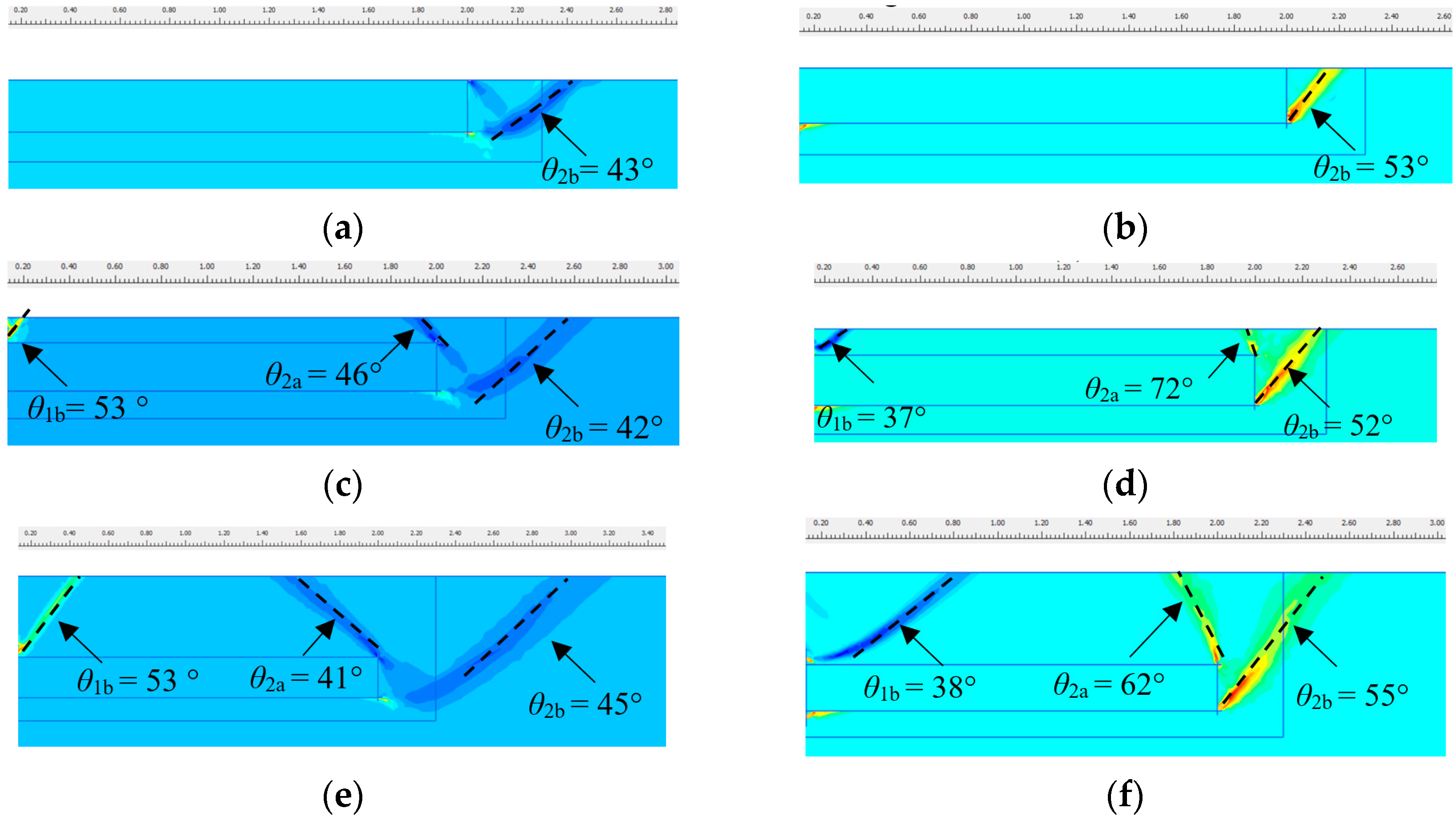
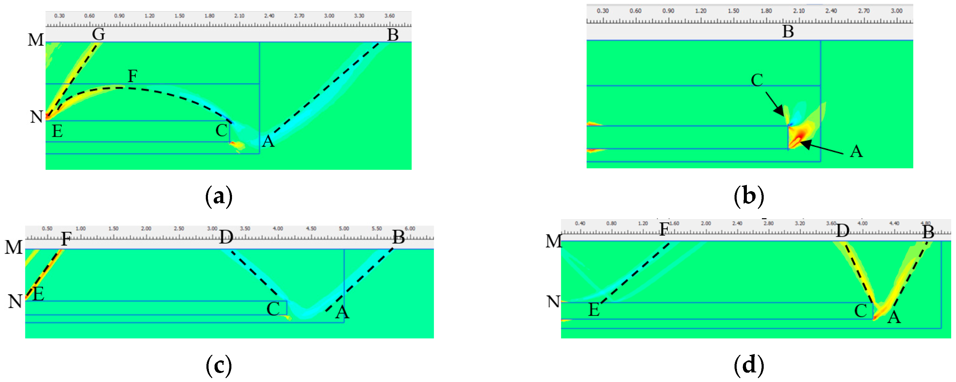
3.2.3. Sand Deformation

The sand deformation of different cases obtained from the FEM is presented in Figure 13. Comparing Figure 10 and Figure 13, it can be found that the differences (δ_v) between the FEM results (v_FEM) and test results (v_TEST) of different cases are basically within 10 mm. When the sand surface uplifts, the differences in w (δ_w) between the FEM results (w_FEM) and test results (w_TEST) of different cases are less than 0.1 m. When the sand surface subsides, δ_w is less than 0.2 m. δ_w in the case of sand subsidence is larger than that in the case of sand uplift. This is probably due to the fact that the sand in the test can subside more readily as discrete particles, while the sand in the FEM has better continuity.

The sand strain contour plots of different cases obtained from the FEM are illustrated in Figure 14. It can be found that there is a continuous plastic zone in the sand after applying displacement and slip surfaces finally appear, indicating a general shear failure mode. The numerical failure mode is in accordance with the experimental sand deformation described in Section 2.5.3. Comparing Figure 10 and Figure 14, it can be found that when the sand surface uplifts, the differences (δ_θ) between the horizontal angle of the slip surface (θ) obtained from the FEM (θ_FEM) and tests (θ_TEST) in different cases are less than 10°. However, when the sand surface subsides, δ_θ of different cases is between 20° and 24°. This may be because the sand moisture content in the test and the FEM is different. In general, the FEM can be used to predict the sand deformation obtained from the test.

3.2.4. Earth Pressure

The peak p (p_u) of different cases were derived based on the locations of the earth pressure measurement points in Figure 5a, as illustrated in Figure 15. Solid and hollow symbols are used to symbolize the p_u obtained from the test (p_u-TEST) and FEM (p_u-FEM), respectively. It is found that the distribution patterns of p_u-FEM and p_u-TEST are similar. Under push u_t, the p_u-FEM of S₄ is the largest, while values at the other measurement points are nearly zero. Under pull u_t, the p_u-FEM of S₅ is the largest, the p_u-FEM values of S₃, S₂, and S₁ decrease gradually, and the p_u-FEM of S₄ is nearly zero. p_u-FEM is larger than p_u-TEST. This may be due to the presence of voids in the sand at the start of the test, which could increase the sand compression space. In contrast, the FEM usually assumes the sand to be a continuous medium without initial voids.

4. Mechanism Analysis of FASSI

4.1. Parametric Analysis

Given L values of 180, 300, and 400 cm and H values of 0 cm, 63 cm, 100 cm, and 132 cm, respectively, the parametric analyses were conducted using the verified FEM in Section 3. The sand deformation and mechanical performance of the FAS specimen under push and pull u_t were investigated. Therefore, twenty-four cases were obtained, detailed information on which is listed in

Table 3. Characteristic points of the F-u curves obtained from FEM with different parameters.

Loading Direction	L (cm)	H (cm)	Labels	k (kN/mm)	Fu (kN)
Push	180	0	L180H0-Push	5.68	6.65
		63	L180H63-Push	15.21	37.17
		100	L180H100-Push	20.15	55.06
		132	L180H132-Push	27.63	99.71
	300	0	L300H0-Push	9.29	24.70
		63	L300H63-Push	18.37	56.60
		100	L300H100-Push	24.51	76.21
		132	L300H132-Push	32.80	129.24
	400	0	L400H0-Push	11.26	40.09
		63	L400H63-Push	20.16	70.88
		100	L400H100-Push	27.58	93.25
		132	L400H132-Push	36.92	160.77
Pull	180	0	L180H0-Pull	7.58	−6.45
		63	L180H63-Pull	21.69	−25.28
		100	L180H100-Pull	35.58	−45.53
		132	L180H132-Pull	55.66	−58.33
	300	0	L300H0-Pull	20.41	−28.66
		63	L300H63-Pull	32.21	−48.03
		100	L300H100-Pull	45.01	−64.62
		132	L300H132-Pull	67.16	−82.73
	400	0	L400H0-Pull	30.29	−45.82
		63	L400H63-Pull	43.99	−61.14
		100	L400H100-Pull	58.29	−78.88
		132	L400H132-Pull	89.37	−97.46

.

In Table 3, the first part of the label (L180, L300, or L400) indicates the slab length of the specimen. The second part of the label (H0, H63, H100, or H132) indicates the embedded depth of the specimen calculated from the sand surface to the lower surface of the FAS specimen. The third part of the label (Push or Pull) indicates the displacement direction. For example, L180H63-Push represents the test case of a FAS specimen with a 180 cm L and a 63 cm H subjected to push u_t. The values of parameters and the F_u, k, and l of corresponding numerical F-u curves of different cases are listed in Table 3.

4.2. Load–Displacement Curve

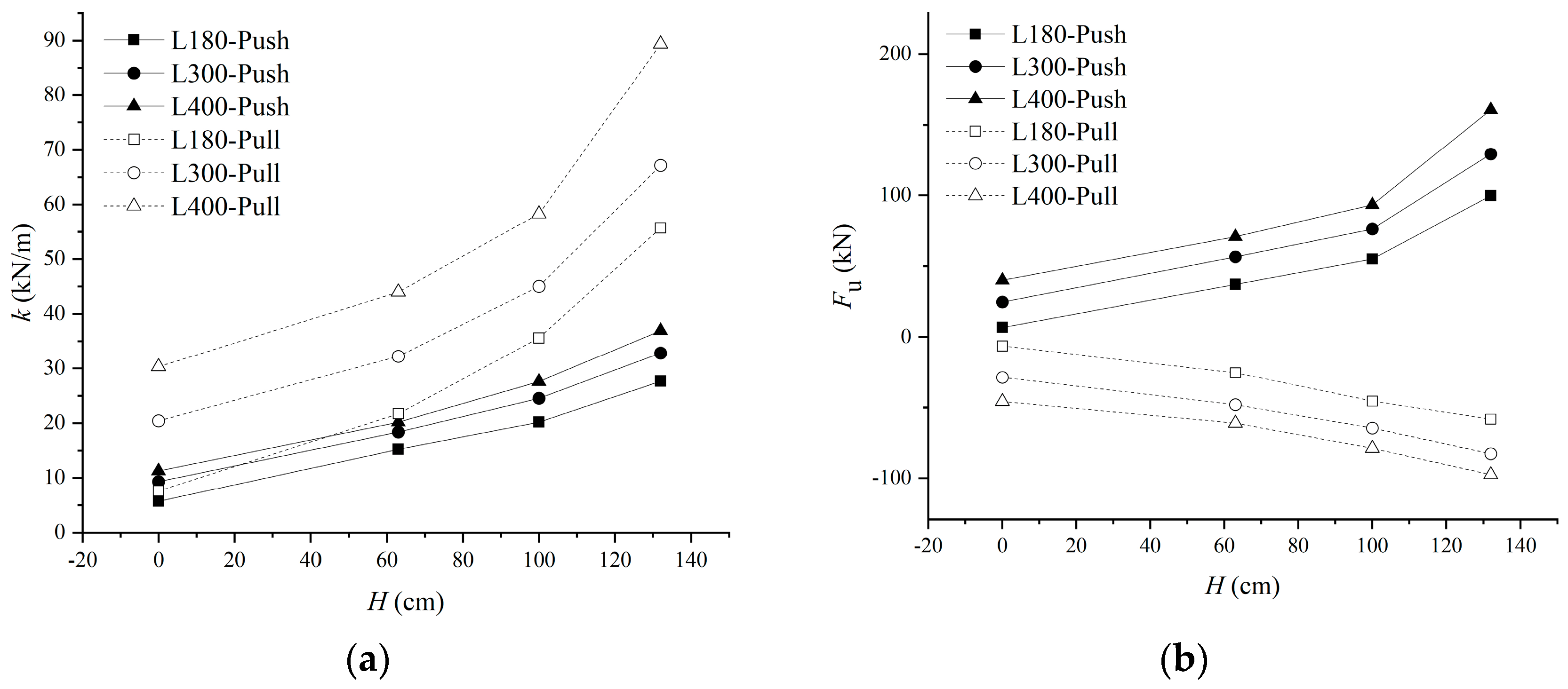
4.2.1. Influence of Embedded Depth

The relationships between H and k, as well as H and F_u, are demonstrated in Figure 16. With an increase in H, k nonlinearly increases, as shown in Figure 16a. When H is the same, k under pull u_t is larger than that under push u_t. Additionally, when the increment in H is the same, the increment in k under pull u_t is larger than that under push u_t. With an increase in H, F_u nonlinearly increases, as shown in Figure 16b. When H is the same, F_u under pull u_t is smaller than that under push u_t. Additionally, when the increment in H is the same, the increment in F_u under pull u_t is smaller than that under push u_t. The influence of the displacement direction on the H–F_u relationship is opposite to that on the H–k relationship. This is due to the following reasons.

When the FAS specimen starts to move and the F-u curve is in the elastic stage, the FAS specimen is subjected to friction between its upper and lower surfaces and the corresponding sand and the earth pressure from the sand at its distal end. With an increase in H, the vertical pressures on the upper and lower surfaces of the FAS specimen increase accordingly, leading to an increment in the friction between the FAS specimen and sand. Meanwhile, with an increase in H, the earth pressure of the sand on the distal end of the FAS specimen increases, contributing to an increment in k. As shown in Figure 10 and Figure 14, the earth pressure distribution zone ABD at the distal end of the FAS specimen is wedge-shaped. Therefore, with an increase in H, the range zone ABD nonlinearly extends, resulting in a nonlinear and rapid increment in k.

Under push u_t, the FAS specimen and the sand above it both move away from the front wall. The earth pressure of the sand at the distal end of the FAS specimen transforms from the static earth pressure to the passive earth pressure. The earth pressure at the distal end of the FAS specimen could restrain the movement of the sand above it. Consequently, the relative sliding between the FAS specimen and the sand could produce friction. Under pull u_t, the FAS specimen and the sand above it move toward the front wall. The earth pressure of the sand at the distal end of the FAS specimen transforms from the static earth pressure to the active earth pressure. The sand above or below the proximal end of the FAS specimen is restrained by the front wall. Consequently, the relative sliding between the FAS specimen and the sand could produce friction. Since the sand above or below the proximal end of the FAS specimen is in direct contact with the fixed front wall, the earth pressure at the distal end of the FAS specimen occurs when the sand is compressed to a certain degree. Therefore, the friction between the FAS specimen and the corresponding sand above and below it in the elastic stage under pull u_t is larger than that under push u_t. As a result, k under pull u_t is larger than that under push u_t.

When the F-u curve is in the failure stage, the slip surfaces of the sand shown in Figure 10 are formed. The passive earth pressure generated by the sand ABD at the distal end of the FAS specimen under push u_t is significantly larger than the active earth pressure under pull u_t. Consequently, F_u under push u_t is notably larger than that under pull u_t. Due to the θ in the slip surface, with an increase in H, the area of sand that is affected by u expands and the increment in F_u under push u_t is larger than that under pull u_t.

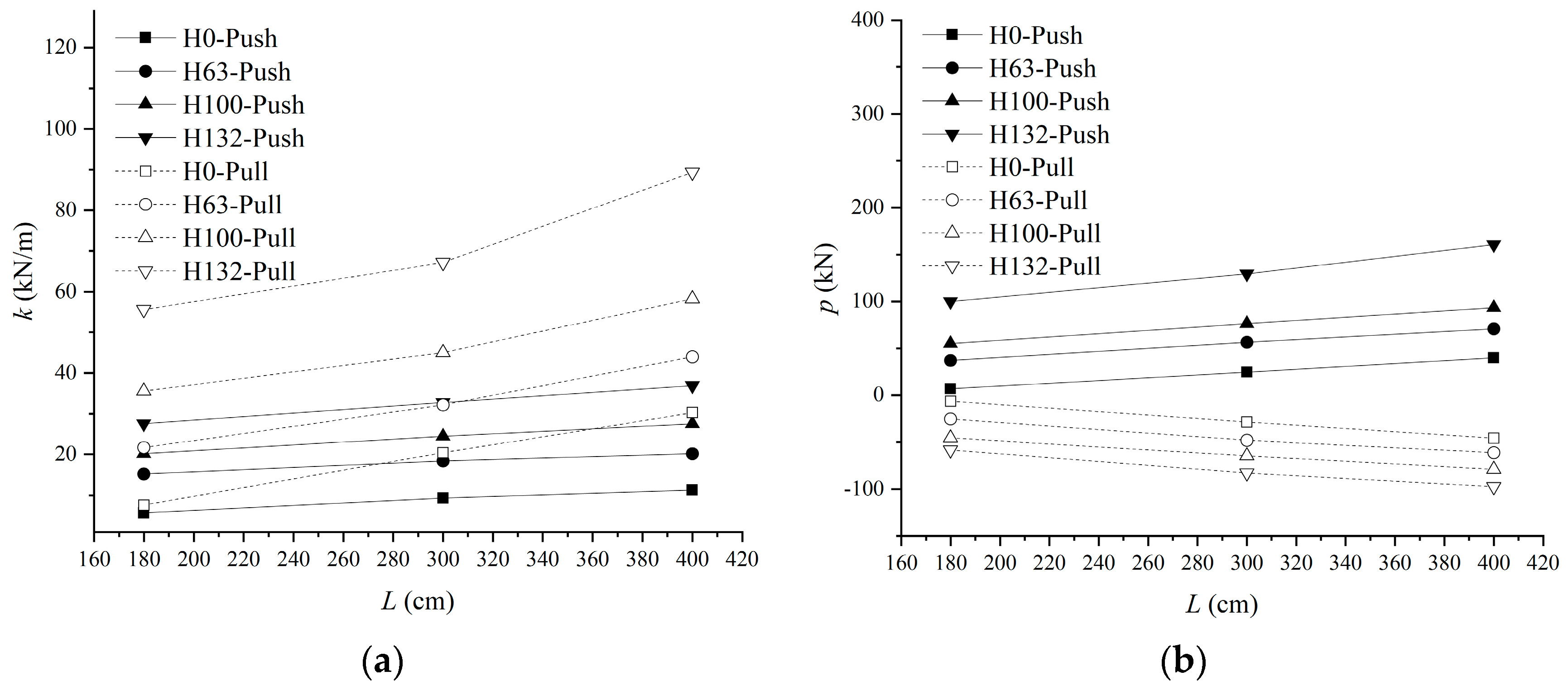
4.2.2. Influence of Slab Length

The relationships between L and k, as well as L and F_u, are demonstrated in Figure 17. With an increase in L, k and F_u nearly linearly increase, as shown in Figure 17a,b. This is because, when the FAS specimen starts to move and the F-u curve is in the elastic stage, the FAS specimen is subjected to friction between its upper and lower surfaces and the corresponding sand and the earth pressure from the sand at its distal end. With an increase in L, the contact surface area on the upper and lower surfaces of the FAS specimen linearly increases, leading to a linear increment in the friction between the FAS specimen and sand and a linear increment in k. When the F-u curve is in the failure stage, the slip surfaces of the sand shown in Figure 10 are formed. The earth pressures produced by the sand zones ABD and EFG located at the distal and proximal ends of the FAS specimen are not affected by the increment in L. Therefore, with an increase in L, the contact surface area on the upper and lower surfaces of the FAS specimen linearly increases, leading to a linear increment in the friction between the FAS specimen and sand and a linear increment in F_u.

When L is the same, k under pull u_t is larger than that under push u_t. With an increase in L, k linearly increases, as shown in Figure 17b. When L is the same, F_u under pull u_t is smaller than that under push u_t. The influence of the displacement direction on the L–F_u relationship is opposite to that on the L–k relationship. The reason for this is similar to that given in Section 4.2.1.

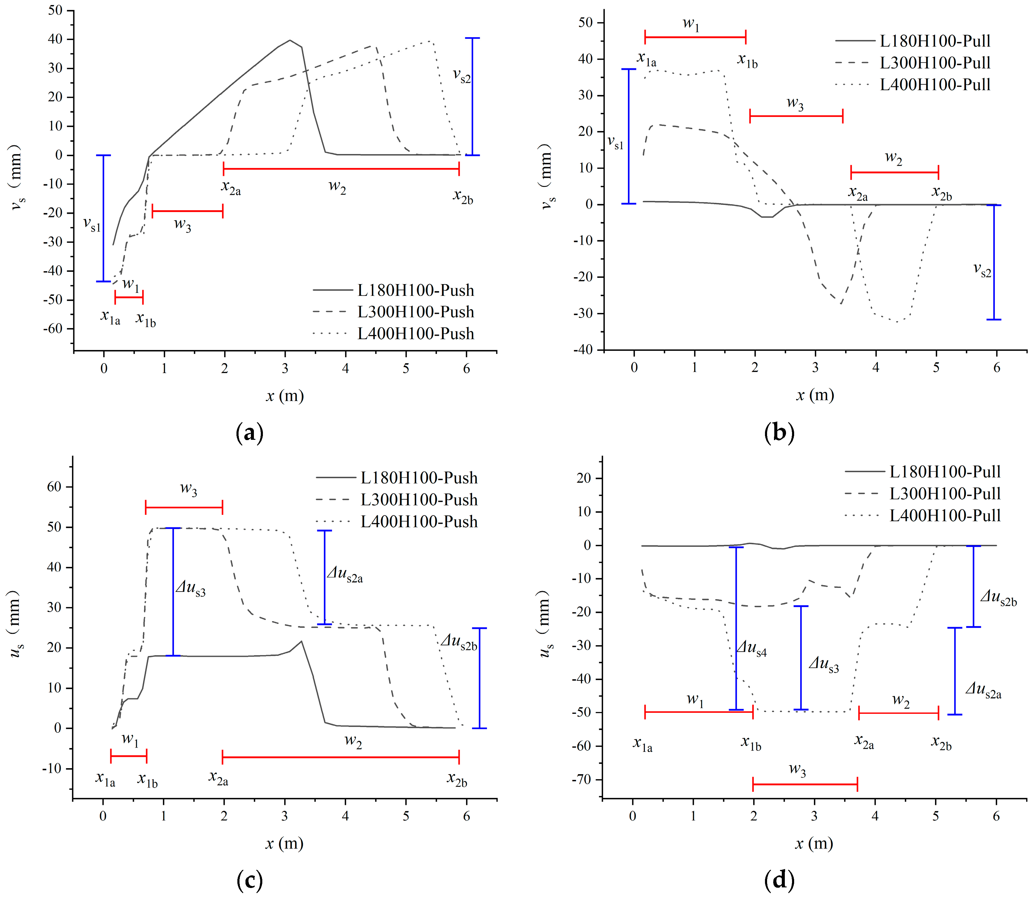
4.3. Sand Deformation

The influence of v_s on the sand surface evenness can be reduced by increasing the u_t absorbed by the FASSI. Due to the limitations in the tests, the longitudinal displacement of the sand (u_s) at different positions (x) of its surface under u_t cannot be measured during the test. The variation in u_s is defined as Δu_s, which can be also considered as the absorption amount of u_t. The absorption of push and pull u_t are defined as positive and negative Δu_s, respectively. The influence of H and L on the longitudinal displacement transfer mode (LDM) and vertical deformation distribution mode (VDM) were analyzed using the FEM.

4.3.1. Influence of Embedded Depth

The sand strain contour plots of the cases with a 300 cm L and different H under push and pull u_t are shown in Figure 18. The black dashed line indicates the slip surface formed by the penetration of plastic strain, and the arrow in Figure 18f indicates the plastic strain concentration area. Points M and N are, respectively, the points on the sand surface and the upper surface of the FAS closest to the bridge, and Points E and C are, respectively, the intersections of the proximal and distal slip surfaces on the upper surface of the FAS. Points G, F, D, and B represent the longitudinal positions (x) at the sand surface, which are x_1a, x_1b, x_2a, and x_2b, respectively.

In addition, the distributions of u_s and v_s at different longitudinal positions (x) of the sand surface obtained from the FEM with different H are shown in Figure 19. The cases with a 63 cm H in Figure 19 were chosen as an example to define the parameters. x_1a denotes the position of the sand surface closest to the bridge; x_1a, x_1b, x_2a, and x_2b denote the positions where v_s is 0; the width between x_1a and x_1b is w₁; the width between x_2a and x_2b is w₂; and the width between x_1b and x_2a is w₃. Moreover, the surface deformation of the cases with different H is listed in

Table 4. Sand surface deformation of cases with different H and L.

Loading Direction	L	H	VDM	vs1	vs2	LDM	Δus2a	Δus2b	Δus3	Δus4
	cm			mm			mm
Push	180	63	VDM1a	−28	41	LDM1a	−24	−26	/	/
	180	100	VDM2a	−27	40	LDM2a	/	−18	−32	/
	180	132	VDM2a	−27	39	LDM2a	/	−12	−38	/
	300	63	VDM1a	−28	42	LDM1a	−24	−26	/	/
	300	100	VDM1a	−45	38	LDM1a	−25	−25	/	/
	300	132	VDM2a	−40	36	LDM2a	/	−21	−29	/
	400	63	VDM1a	−28	40	LDM1a	−24	−26	/	/
	400	100	VDM1a	−42	39	LDM1a	−25	−25	/	/
	400	132	VDM1a	−43	35	LDM1a	−24	−26	/	/
Pull	180	63	VDM2b	41	−35	LDM2b	5	15	30	/
	180	100	VDM3b	1	−3	LDM3b	/	1	/	49
	180	132	VDM3b	1	−2	LDM3b	/	1	/	49
	300	63	VDM1b	41	−36	LDM1b	27	23	/	/
	300	100	VDM2b	23	−27	LDM2b	6	12	32	/
	300	132	VDM3b	−1	−2	LDM3b	/	1	/	49
	400	63	VDM1b	41	−35	LDM1b	25	25	/	/
	400	100	VDM1b	36	−32	LDM1b	27	23	/	/
	400	132	VDM2b	9	−12	LDM2b	3	5	42	/

.

• Under push displacement:

When H is 63 cm, the sand slip surfaces CD and AB at the distal end of the FAS specimen and the sand slip surface EF at its proximal end are illustrated in Figure 18a. As shown in Figure 19a, the sand in w₁ subsides with a maximum v_s (v_s1) of −28 mm; the sand in w₂ uplifts, with a maximum v_s (v_s2) of 42 mm; and v_s within w₃ is essentially 0 mm. This is because the sand zone ABD is in compression and the sand zone EFMN is in tension, as shown in Figure 18a. This kind of VDM can be set as VDM_1a. u_s in w₃ equals u_t, indicating that the sand zone EFDC moves along with the FAS specimen. As shown in Figure 18a, two absorption points of u_t (x_2a and x_2b) can be found at points D and B, and the corresponding Δu_s values are Δu_s2a = −24 mm and Δu_s2b = −26 mm, respectively. u_t reduces to zero at x_2b, indicating that the sand surface away from x_2b is not affected by u_t. This kind of LDM can be set as LDM_1a and expressed as u_t = Δu_s2a + Δu_s2b.

When H is 100 cm, the sand strain contour plot as shown in Figure 18c is nearly the same as that with a 63 cm H as shown in Figure 18a. When H changes from 63 cm to 100 cm, the VDM and LDM are nearly the same as shown in Figure 19a,c, however, v_s1 increases by 17 mm and v_s2 decreases by 4 mm. This is because, when H changes from 63 cm to 100 cm, with an increase in H, the sand voids that occur in the sand zone EFMN increase in size leading to an increase in v_s1, At the same time, the volume of the sand zone ABD increases leading to a larger displacement absorption and a decrease in v_s2.

When H is 132 cm, the VDM and LDM are different from those of the cases with a 63 cm or 100 cm H. The sand slip surfaces EF and AB are formed at the proximal and distal ends of the FAS specimen, as shown in Figure 18e. As shown in Figure 19a, the sand in w₁ subsides, while the sand in w₂ and w₃ both uplift. This is because the sand zone EGMN in Figure 18e is in tension, and the sand zone GEFCAB is in compression. This kind of VDM can be set as VDM_2a. Compared with VDM_1a of the case with a 100 cm H, v_s1 and v_s2 of VDM_2a in the case with a 132 cm H are reduced by 5 mm and 2 mm, respectively. A displacement absorption zone l_GB for u_t between Points G and B in Figure 18e can be found, as shown in Figure 19c. u_s within w₂ and w₃ decreases by a Δu_s3 of 29 mm relative to u_t, indicating that the sand within w₂ and w₃ has a relative movement with the FAS specimen. A displacement absorption point x_2b at Point B in Figure 18e can absorb the Δu_s of 21 mm at x_2b (Δu_s2b), and then u_t decreases to zero. This kind of LDM can be set as LDM_2a and expressed as u_t = Δu_s3 + Δu_s2a + Δu_s2b (Δu_s2a = 0). When H changes from 100 cm to 132 cm, the LDM changes from LDM_1a to LDM_2a, Δu_s3 is absorbed by the displacement absorption zone l_GB, which will reduce u_t absorbed by the sand zone EGMN and the corresponding v_s1. Simultaneously, since u_t absorbed by Δu_s2b relatively decreases, the deformation of the sand zone GEFCAB is reduced, leading to a decrease in v_s2.

• Under pull displacement:

When H is 63 cm, the sand slip surfaces under pull u_t, as illustrated in Figure 18b, are similar to those of the cases with a 63 cm or 100 cm H under push u_t, as shown in Figure 18a. For the case with a 63 cm H under pull u_t, the sand in w₁ uplifts, with a v_s1 of 41 mm; the sand in w₂ subsides, with a v_s2 of −36 mm; v_s within w₃ is essentially 0 mm. This is because the sand zone EFMN is in compression and the sand zone ABD is in tension, as shown in Figure 19b. Therefore, the VDM of the case with a 63 cm H under pull u_t can be set as VDM_1b. u_s in w₃ equals u_t, indicating that the sand zone EFDC moves along with the FAS specimen. As shown in Figure 18b, two absorption points of u_t (x_2a and x_2b) can be found at Points D and B, and the corresponding Δu_s are Δu_s2a = 24 mm and Δu_s2b = 26 mm, respectively. u_t reduces to zero at x_2b, indicating that the sand surface away from x_2b is not affected by u_t. This kind of LDM can be set as LDM_1b and expressed as u_t = Δu_s2a + Δu_s2b. The sand deformation ranges of the VDM_1b and LDM_1b are similar to those of VDM_1a and LDM_1b, respectively, with the opposite parameter values.

The VDM and LDM of the case with a 100 cm H under pull u_t are different from those of the case with a 63 cm H, as shown in Figure 19b. The sand slip surface EF is formed at the proximal end of the FAS specimen and the sand slip surfaces CF and AB are formed at the distal end of the FAS specimen, as shown in Figure 18d. The sand in w₁ and w₃ both uplift; and the sand in w₂ subsides. This is because the sand zones EGMN and EFCDG in Figure 18d are in compression and the sand zone ABD is in tension. This kind of VDM can be set as VDM_2b. Compared with VDM_1b of the case with a 63 cm H, v_s1 and v_s2 of VDM_2b in the case with a 100 cm H are reduced by 19 mm and 9 mm, respectively. A displacement absorption zone l_GB for u_t between Points G and B in Figure 18d can be found, as shown in Figure 19d. u_s within w₁ and w₃ decreases by a Δu_s3 of 32 mm relative to u_t. Two absorption points of u_t (x_2a and x_2b) can be found at Points D and B, and the corresponding Δu_s areΔu_s2a = 21 mm and Δu_s2b = 11 mm, respectively. u_t reduces to zero at x_2b, indicating that the sand surface away from x_2b is not affected by u_t. This kind of LDM can be set as LDM_2b and expressed as u_t = Δu_s3 + Δu_s2a + Δu_s2b. The sand deformation ranges of VDM_2b are similar to those of VDM_2a. v_s1 and v_s2 of VDM_2b are opposite to those of VDM_2a. Δu_s2a of LDM_2b is not zero due to the sand slip surface CD, which is different from Δu_s2a of LDM_2a. When H changes from 63 cm to 100 cm, the LDM changes from LDM_1b to LDM_2b, the volume of the sand zones EGMN, EFCDG, and ABD, and the corresponding displacement absorption increase. Moreover, Δu_s3 is absorbed by the displacement absorption zone l_GB, which will reduce u_t absorbed by the sand zone EGMN and the corresponding v_s1. Simultaneously, since u_t absorbed Δu_s2a and Δu_s2b relatively decreases, the deformation of the sand zone EFCDG is reduced, leading to a decrease in v_s2.

The VDM and LDM of the case with a 132 cm H under pull u_t are different from those of the cases with a 63 cm or 100 cm H, as shown in Figure 19b. The sand surfaces in w₁ and w₃ do not change and the sand in w₂ subsides. This kind of VDM can be set as VDM_3b. Compared with VDM_2b of the case with a 100 cm H, v_s1 and v_s2 of VDM_3b in the case with a 132 cm H are reduced by 22 mm and 25 mm, respectively. u_s decreases by a Δu_s4 of 50 mm relative to u_t, which nearly equals u_t, as shown in Figure 19c. Relative sliding is observed between the FAS specimen and the sand. An absorption point of u_t (x_2b) can be found at Point C, and the corresponding Δu_s is Δu_s2b = 1 mm. u_t reduces to zero at x_2b, indicating that the sand surface away from x_2b is not affected by u_t. This kind of LDM can be set as LDM_3b and expressed as u_t = Δu_s4 + Δu_s2b. VDM_3b and LDM_3b are due to the fact that the plastic strains at Points A and C do not extend to the sand surface, as shown in Figure 18f. u_t is reduced by Δu_s4 due to the relative sliding between the FAS specimen and the sand. Meanwhile, local voids generated at the end of the FAS specimen lead to the subsidence of Point B directly above it and the reduction of u_t by Δu_s2b. Therefore, the u_s reflected to the sand surface is so small that the v_s on the sand surface is hardly noticeable.

4.3.2. Influence of Slab Length

The sand strain contour plots of the cases with a 100 cm H and different L (180 or 400 cm) under push and pull u_t are shown in Figure 20. The sand strain contour plots of the cases with a 100 cm H and a 300 cm L under push and pull u_t are illustrated in Figure 18c,d. The distributions of u_s and v_s at different longitudinal positions (x) of the sand surface obtained from the FEM with different L are shown in Figure 21. The definitions of the points and symbols in Figure 20 and Figure 21 are the same as those in Figure 18 and Figure 19 of Section 4.3.1, respectively. Moreover, the surface deformation of the cases with different L are listed in Table 4.

• Under push displacement:

When L is 180 cm, the sand slip surfaces in the sand strain contour plot shown in Figure 20a are nearly the same as those of L300H132-Push in Figure 18e. The VDM of the case with a 180 cm L can be set as VDM_2a. v_s1 is −27 mm and v_s2 is 40 mm, as shown in Figure 21a. The LDM of the case with a 180 cm L can be set as LDM_2a, with a Δu_s2b of −18 mm and a Δu_s3 of −32 mm, as shown in Figure 21c;

As introduced in Section 4.3.1, the VDM and LDM of the cases with a 300 cm L under push u_t are VDM_1a and LDM_1a, respectively. Compared with the VDM and LDM of the cases with a 180 cm L, v_s1 increases by 18 mm and v_s2 decreases by 2 mm, as shown in Figure 21a; Δu_s2a increases by 24 mm, Δu_s2b decreases by 6 mm, and Δu_s3 decreases to 0 mm, as shown in Figure 21c;

When L is 400 cm, the sand slip surfaces in the sand strain contour plot shown in Figure 20c are nearly the same as those of L300H100-Push in Figure 18c. The VDM and LDM of the case with a 400 cm L is also VDM_1a and LDM_1a. Compared with the VDM and LDM of the cases with a 300 cm L, v_s1 decreases by 3 mm and v_s2 increases by 1 mm, as shown in Figure 21a; the variations in Δu_s2a and Δu_s2b are less than 1 mm, as shown in Figure 21c. This is because the sand deformation of sand zones EFMN, ABD, and EFG located at the distal and proximal ends of the FAS specimen are not affected by the increment in L.

• Under pull displacement:

When L is 180 cm, the sand slip surfaces in the sand strain contour plot shown in Figure 20b are nearly the same as those of L300H132-Pull in Figure 18f. The VDM of the case with a 180 cm L can be set as VDM_3b. v_s1 is −1 mm and v_s2 is −3 mm, as shown in Figure 21b. The LDM of the case with a 180 cm L can be set as LDM_3b, with a Δu_s2b of 1 mm and a Δu_s4 of 49 mm, as shown in Figure 21d;

As introduced in Section 4.3.1, the VDM and LDM of the cases with a 300 cm L under pull u_t are VDM_2b and LDM_2b, respectively. Compared with the VDM and LDM of the cases with a 180 cm L, v_s1 and v_s2 increase by 22 mm and 24 mm, respectively, as shown in Figure 21b; Δu_s2a, Δu_s2b, and Δu_s3 increase by 6 mm, 12 mm, and 32 mm, respectively, and Δu_s4 decreases to 0 mm, as shown in Figure 21d;

When L is 400 cm, the sand slip surfaces in the sand strain contour plot shown in Figure 20d are nearly the same as those of L300H100-Pull in Figure 18d. The VDM and LDM of the case with a 400 cm L are also VDM_1b and LDM_1b. Compared with the VDM and LDM of the cases with a 300 cm L, v_s1 increases by 14 mm and v_s2 decreases by 5 mm, as shown in Figure 21b; Δu_s2a and Δu_s2b increase by 21 mm and 11 mm, respectively, and Δu_s3 decreases to 0 mm, as shown in Figure 21d.

The analyses conducted in Section 4.2 and Section 4.3 show that with an increase in H, the LDM changes from LDM_1a to LDM_2a under push u_t and from LDM_1b to LDM_3b under pull u_t. With an increase in L, the LDM changes from LDM_2a to LDM_1a under push u_t and from LDM_3b to LDM_1b under pull u_t. It can be concluded that the influence of H on the LDM of FASSI is opposite to the influence of L on the LDM of FASSI. Consequently, with an increase in H or a decrease in L, Δu_s2a and Δu_s2b on the sand surface decrease, which is beneficial for avoiding pavement crack risks; v_s1 and v_s2 also decrease, which can improve the pavement evenness. Furthermore, a reduction in slab length can further lower the construction cost. However, when L is too small, it cannot meet the structural requirements. According to [31,32], the minimum L can be taken as twice the height of the abutment.

Furthermore, based on different types of LDM, techniques to reduce the risk of pavement cracking can be proposed. For LDM_1a or LDM_1b, it is suggested to arrange geogrids at Points B and D as illustrated in Figure 18a,b. For LDM_2a or LDM_2b, it is suggested to arrange geogrids in sand zone GEFDAB in Figure 18d,e to avoid the sand slip surface CFE, which could reduce the bearing capacity of the embankment. For LDM_3b, materials with a lower friction coefficient should be used on the upper and lower surfaces of the FAS specimen to increase the relative sliding between the FAS specimen and the sand. Additionally, elastic materials should be filled at the end of the FAS specimen to prevent pavement settlement and subsidence caused by voids.

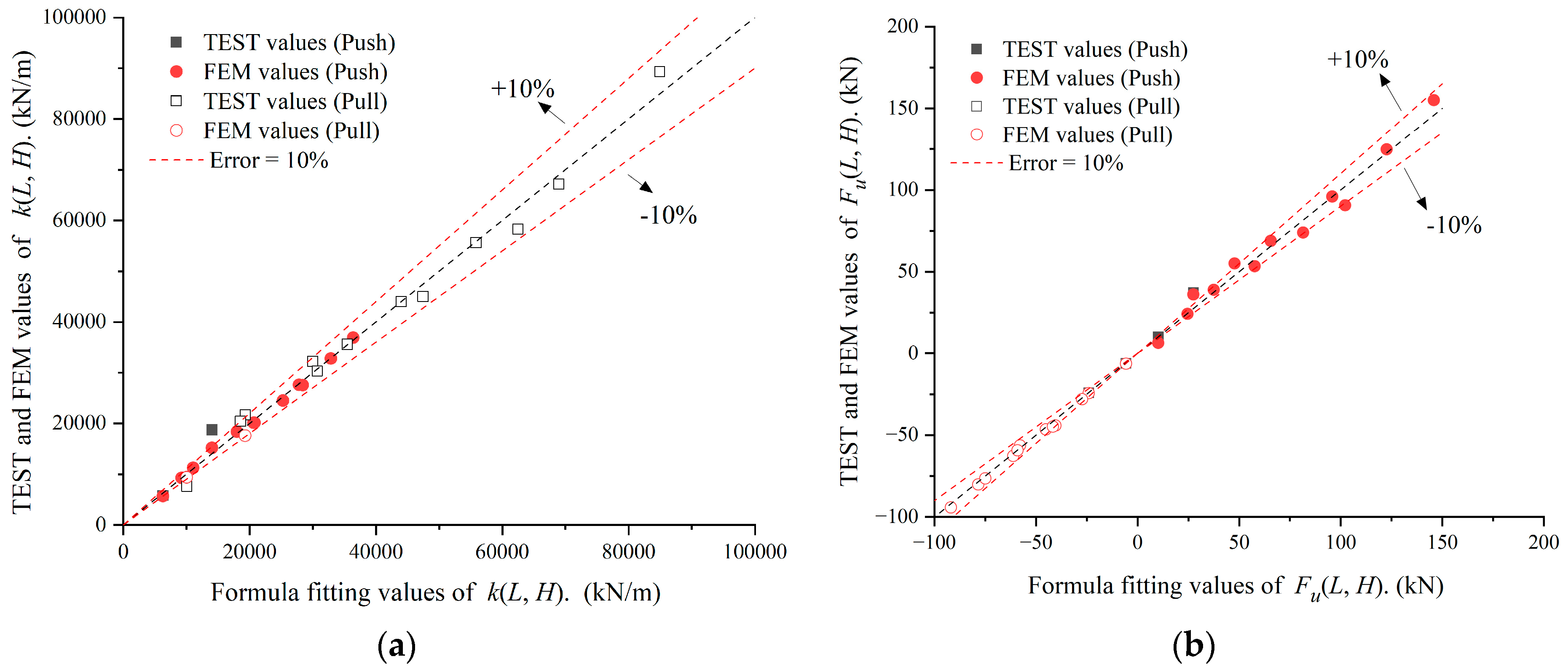
5. Simplified Calculation Formula for Load–Displacement Curve

As mentioned in Section 2.5.2, l is close to 0. The bilinear model composed of two line segments is simple in calculation and can accurately capture the characteristics of the F-u curves of the FASSI both in the elastic stage and failure stage. Therefore, the F-u curves of different cases were simplified by using the bilinear model F(k, F_u, u), which is shown in Figure 22 and can be calculated by using Equation (3). In addition, F(k, F_u, u) is applied when sand is employed as backfill and F is loaded as monotonic. Based on the F_u and k values obtained from numerical F-u curves of the cases with different H and L as listed in Table 3, F_u and k can be set as a function of H and L, namely k(H, L) and F_u(H, L).

$$F\left(k,F_{\mathrm{u}} ,u\right)=\left\{\begin{array}{ll}k·u,& 0\le x<u_0\\ \hfill F_{\mathrm{u}},\hfill & x\ge u_0\end{array}\right.$$

(3)

where u₀ at the intersection of the two lines, which can be calculated by F_u/k.

The influence of H and L on k and F_u are illustrated in Figure 16 and Figure 17. It can be observed that the influence of H and L on k and F_u are nonlinear. Consequently, three-dimensional nonlinear surface fitting was employed, which is in the form of a binary quadratic polynomial, namely Z = Z₀ + ax + by + cx² + dy² + fxy. The three-dimensional surface fitting results of the functions k(H, L) and F_u(H, L) under push and pull displacements are shown in Figure 23.

The fitting formula are Formulas (4)–(7), with R-squared values larger than 0.95, indicating good fitting results.

k_push (H, L) = 203.88 + 39.09L + 63.38H − 0.03L² + 0.58H² + 0.13LH

(4)

F_u.push (H, L) = −9.21 + 0.10L − 0.21H + 4.15 − 5L² + 0.00544H² + 0.000784LH

(5)

k_pull(H, L) = 9665.04 − 39.44L − 87.92H + 0.23L² + 2.90H² + 0.29LH

(6)

F_u.pull(H, L) = 35.66 − 0.26L − 0.21H + 0.000166L² − 0.0015H² + 0.000069LH

(7)

The calculated k and F_u obtained from the simplified calculation formula were compared with the experimental and numerical values obtained from the tests and FEM to verify the accuracy of the simplified calculation formula, as shown in Figure 24.

It can be observed that the error of most points is within 10%. It can be concluded that the simplified calculation formula is accurate enough to meet engineering application requirements.

6. Conclusions

The mechanism of the FASSI with different embedded depths and slab lengths was investigated by using experimental tests, finite element simulations, parametric analyses, and a proposed simplified calculation formula. The main conclusions that can be drawn are as follows:

• The load–displacement curves of FASSI under push or pull displacement can be divided into three stages: the elastic stage, the elastoplastic stage, and the failure stage. In the elastic stage, the longitudinal displacement of a FAS can be absorbed by the sand and no obvious cracks or deformations can be observed on the sand surface. In the elastoplastic stage, part of the sand enters the plastic deformation stage, and bumps and voids can be observed on the sand surface. In the failure stage, a through-going shear slip surface is formed, leading to an overall shear failure of the sand.
• Under push displacement, the sand at the distal end of the approach slab is in a passive state and uplifted to form a bump due to compression; the sand at the proximal end of the approach slab is in an active state and subsides to form a void due to tension. Under pull displacement, the deformations of the sand at the distal and proximal ends of the approach slab are opposite to those under pull displacement. The pavement deformation can be reduced with an increase in the embedded depth, which could reduce the risk of pavement settlement and cracking.
• With an increase in the embedded depth or slab length, the stiffness and ultimate load of the load–displacement curves of FASSI increase under push displacement, the stiffness increases and the ultimate load decreases under pull displacement.
• The longitudinal displacement transfer mode and vertical deformation distribution mode of FASSI are affected by the embedded depth and slab length. With an increase in the embedded depth or a decrease in the slab length, the sand deformation on its surface decreases, which is beneficial for avoiding pavement crack risks and improving pavement evenness.
• A simplified calculation formula that can be used to predict the load–displacement curves of FASSI based on a bilinear function model was proposed by considering the embedded depth and slab length as the parameters. The functions for the embedded depth and slab length were obtained through three-dimensional surface fitting.

This research forms the basis for more in-depth investigations on FASSI under cyclic load in jointless bridges. Based on the authors’ experience of systems at different depths under cyclic load, with an increase in the embedded depth, the ductility and energy dissipation capacity of FASSI may be improved. In future research, the influence of the cyclic load and the different soil properties on FASSI will be investigated in detail through experimental tests.

References

1. Liu, G. Structural Behavior of Integral Abutment Bridge Approach Slabs. Ph.D. Dissertation, University of Illinois at Urbana-Champaign, Champaign, IL, USA, 2023. [Google Scholar]
2. Aloisio, A.; Pelliciari, M.; Xue, J.; Fragiacomo, M.; Briseghella, B. Effect of Pre-Hole Filled with High-Damping Material on the Inelastic Response Spectrum of Integral Abutment Bridges. J. Earthq. Eng. 2023, 27, 3319–3340. [Google Scholar] [CrossRef]
3. Hassan, M.S.K.; Liyanapathirana, D.S.; Fuentes, W.; Leo, C.J.; Hu, P. A review of soil deformation and lateral pressure ratcheting phenomena in integral abutment bridges. Transp. Geotech. 2024, 49, 101388. [Google Scholar] [CrossRef]
4. White, D.; Sritharan, S.; Suleiman, M.T.; Chetlur, S. Identification of the Best Practices for Design, Construction, and Repair of Bridge Approaches; No. CTRE Project 02-118; Iowa Department of Transportation: Ames, IA, USA, 2005. [Google Scholar]
5. White, D.J.; Mekkawy, M.M.; Sritharan, S.; Suleiman, M.T. “Underlying” causes for settlement of bridge approach pavement systems. J. Perform. Constr. Facil. 2007, 21, 273–282. [Google Scholar] [CrossRef]
6. Ahmad, I.; Shokouhian, M. Promoting Sustainable Green Infrastructure: Experimental and Numerical Investigation of Concrete Reinforced with Recycled Steel Fibers. Arch. Adv. Eng. Sci. 2024, 1–13. [Google Scholar] [CrossRef]
7. Erarslan, N.; Şen, B. The Analysis of Liquefaction Potential and Post-Liquefaction Deformations at a Highway Bridge Crossing. Arch. Adv. Eng. Sci. 2023, 1–9. [Google Scholar] [CrossRef]
8. Xue, J.; Aloisio, A.; Lin, Y.; Fragiacomo, M.; Briseghella, B. Optimum design of piles with pre-hole filled with high-damping material: Experimental tests and analytical modelling. Soil Dyn. Earthq. Eng. 2021, 151, 106995. [Google Scholar] [CrossRef]
9. Hoppe, E.; Weakley, K.; Thompson, P. Jointless Bridge Design at the Virginia Department of Transportation. Transp. Res. Procedia 2016, 14, 3943–3952. [Google Scholar] [CrossRef]
10. Breña, S.F.; Bonczar, C.H.; Civjan, S.A.; DeJong, J.T.; Crovo, D.S. Evaluation of seasonal and yearly behavior of an integral abutment bridge. J. Bridge Eng. 2007, 12, 296–305. [Google Scholar] [CrossRef]
11. Prakash, B.; Tiwari, A.K.; Dash, S.R.; Patra, S. Structural evaluation and performance based optimization of approach slab design for mitigating bridge approach settlement through an Indian case study. Structures 2024, 60, 105864. [Google Scholar] [CrossRef]
12. Arockiasamy, M.; Butrieng, N.; Sivakumar, M. State-of-the-Art of Integral Abutment Bridges: Design and Practice. J. Bridge Eng. 2004, 9, 497–506. [Google Scholar] [CrossRef]
13. Wasserman, E.P. Integral abutment design (practices in the United States). In Proceedings of the 1st US-Italy Seismic Bridge Workshop, Pavia, Italy, 18–20 April 2007. [Google Scholar]
14. Connal, J. Integral abutment bridges: Australian and US practice. In Proceedings of the Austroads Bridge Conference, Hobart, Australia, 19–24 May 2004. No. AP-G79/04. [Google Scholar]
15. Ala, N. Seamless Bridge System for the US Practice. Ph.D. Dissertation, University of Nebraska-Lincoln, Lincoln, NE, USA, 2011. [Google Scholar]
16. Puppala, A.J.; Saride, S.; Archeewa, E.; Hoyos, L.R.; Nazarian, S. Recommendations for Design, Construction, and Maintenance of Bridge Approach Slabs: Synthesis Report. 2009. Available online: https://library.ctr.utexas.edu/hostedpdfs/uta/0-6022-1.pdf (accessed on 10 December 2024).
17. Xia, Y.; Cheng, Y. Research on differential settlement characteristics of high fill embankment on expressway. Highw. Eng. 2019, 4, 268–273. [Google Scholar]
18. Akiyama, H.; Kajikawa, Y. Fundamentally Structural Characteristics of Integral Bridges. Ph.D. Dissertation, Kanzawa University, Kanazawa, Japan, 2008. [Google Scholar]
19. Hoppe, E.J. Guidelines For the Use, Design, and Construction of Bridge Approach Slabs; Virginia Department of Transportation: Richmond, VA, USA, 1999. [Google Scholar]
20. Kunin, J.; Alampalli, S. Integral Abutment Bridges: Current Practice in United States and Canada. J. Perform. Constr. Facil. 2000, 14, 104–111. [Google Scholar] [CrossRef]
21. Tabatabai, H.; Oesterle, R.G.; Lawson, T.J. Jointless Bridges, Experimental Research and Field Studies; Report Submitted to the Federal Highway Administration: Washington, DC, USA, 2005; Volume I. [Google Scholar]
22. Maruri, R.F.; Petro, S.H. Integral Abutments and Jointless Bridges (IAJB) 2004 Survey Summary; Federal Highway Administration West Virginia Department of Transportation: Washington, DC, USA, 2005. [Google Scholar]
23. Lin, Z.; Peng, D. Influence of Approach Plate on Mechanical Performance of Bridges Without Expansion Joints. In Proceedings of the 13th National Conference on Structural Engineering, Vancouver, BC, Canada, 1–6 August 2004; Volume II. [Google Scholar]
24. Xue, J.Q.; Tang, Y.F.; Briseghella, B.; Huang, F.Y.; Nuti, C. Experimental Study on SSI of Flat Buried Approach Slab in Jointless Bridge. In Bridge Maintenance, Safety, Management, Life-Cycle Sustainability and Innovations; CRC Press: Boca Raton, FL, USA, 2021. [Google Scholar]
25. Briseghella, B.; Tang, Y.F.; Xue, J.Q.; Chen, B.C.; Huang, F.Y. Review of research on approach slabs in jointless bridges. J. Fuzhou Univ. (Nat. Sci. Ed.) 2021, 49, 209–216. [Google Scholar]
26. Prakash, B.; Tiwari, A.K.; Dash, S.R. Bridge Approach Settlement and its Mitigation Schemes: A Review. Transp. Res. Rec. J. Transp. Res. Board 2024, 2678, 660–689. [Google Scholar] [CrossRef]
27. Reza, F. Synthesis of Bridge Approach Panels Best Practices; No. MN/RC 2013-09. 2013. Available online: https://mdl.mndot.gov/_flysystem/fedora/2023-01/201309.pdf (accessed on 10 December 2024).
28. Ala, N.; Azizinamini, A. Proposed design provisions for a seamless bridge system: Cases of flexible and jointed pavements. J. Bridge Eng. 2016, 21, 04015045. [Google Scholar] [CrossRef]
29. Lu, Q.; Li, M.; Gunaratne, M.; Xin, C.; Hoque, M.; Rajalingola, M. Best Practices for Construction and Repair of Bridge Approaches and Departures. 2018. Available online: https://rosap.ntl.bts.gov/view/dot/35511 (accessed on 10 December 2024).
30. White, H.; Pétursson, H.; Collin, P. Integral abutment bridges: The European way. Pract. Period. Struct. Des. Constr. 2010, 15, 201–208. [Google Scholar] [CrossRef]
31. Wendner, R.; Strauss, A. Inclined Approach Slab Solution for Jointless Bridges: Performance Assessment of the Soil-Structure Interaction. J. Perform. Constr. Facil. 2015, 29, 04014045. [Google Scholar] [CrossRef]
32. Phares, B.M.; Faris, A.S.; Greimann, L.; Bierwagen, D. Integral bridge abutment to approach slab connection. J. Bridge Eng. 2013, 18, 179–181. [Google Scholar] [CrossRef]
33. Tang, Y.; Briseghella, B.; Xue, J.; Zhang, P.; Huang, F. Research on friction between grade flat approach slab and sliding material in jointless bridges. In Proceedings of the 20th Congress of IABSE, New York, NY, USA, 4–6 September 2019; The Evolving. Metropolis-Report. International Association for Bridge and Structural Engineering (IABSE): Zurich, Switzerland, 2019; pp. 959–963. [Google Scholar]
34. Jin, X. Design and Experimental Research on a New Fully Jointless Bridge System. Ph.D. Dissertation, Hunan University, Changsha, China.
35. Jin, X.; Shao, X. A study of fully jointless bridge-approach system with semi-integral abutment. J. Civ. Eng. 2009, 9, 68–73. [Google Scholar]
36. Burdet, O.; Einpaul, J.; Muttoni, A. Experimental Investigation of Soil-structure Interaction for the Transition Slabs of Integral Bridges. Struct. Concr. 2016, 16, 470–479. [Google Scholar] [CrossRef]
37. D’Amato, M.; Laterza, M.; Casamassima, V.I.T.O. Seismic performance evaluation of a multi-span existing masonry arch bridge. Open Civ. Eng. J. 2017, 11, 1191–1207. [Google Scholar] [CrossRef]
38. Rota, M.; Pecker, A.; Bolognini, D.; Pinho, R. A methodology for seismic vulnerability of masonry arch bridge walls. J. Earthq. Eng. 2005, 9, 331–353. [Google Scholar] [CrossRef]
39. Fahnestock, L.A.; Chee, M.; Liu, G.; Kode, U.; LaFave, J.M. Synthesis of Bridge Approach Slab Behavior, Design, and Construction Practice. Pract. Period. Struct. Des. Constr. 2023, 27, 04022032. [Google Scholar] [CrossRef]
40. Abo El-Khier, M.; Morcous, G. Design and Detailing of Bridge Approach Slabs: Cast-in-Place and Precast Concrete Options. In Sustainable Issues in Infrastructure Engineering: The Official 2020 Publication of the Soil-Structure Interaction Group in Egypt (SSIGE); Springer International Publishing: Berlin/Heidelberg, Germany, 2021; pp. 193–206. [Google Scholar]
41. Tang, Y.; Briseghella, B.; Xue, J.; Huang, F.; Chen, B.; Nuti, C. Numerical Analysis of the Mechanical Behaviors of Girders in Jointless Bridge Considering the Grade Flat Approach Slab. In Life-Cycle Civil Engineering: Innovation, Theory and Practice; CRC Press: Boca Raton, FL, USA, 2021; pp. 1486–1491. [Google Scholar]
42. Slavinska, O.; Andriy, B.; Ihor, K.; Oleksandr, D. Estimation of the Service Life of Approach Slabs of Road Bridges Based on the Statistical Modeling Method. Tehnički Glasnik 2024, 18, 618–625. [Google Scholar] [CrossRef]
43. Fu, R.H.; Briseghella, B.; Xue, J.-Q.; Aloisio, A.; Lin, Y.-B.; Nuti, C. Experimental and Finite Element Analyses of Laterally Loaded RC Piles with Pre-Hole Filled by Various Filling Materials in IABs. Eng. Struct. 2022, 272, 114991. [Google Scholar] [CrossRef]
44. Lombardi, D.; Bhattacharya, S.; Scarpa, F.; Bianchi, M. Dynamic Response of a Geotechnical Rigid Model Container with Absorbing Boundaries. Soil Dyn. Earthq. Eng. 2015, 69, 46–56. [Google Scholar] [CrossRef]
45. Dreier, D. Interaction Sol-Structure Dans Le Domaine Des Ponts Intégraux; EPFL: Lausanne, Switzerland, 2010. [Google Scholar]
46. GB50021-2001; Code for Geotechnical Investigation. Ministry of Construction of the People’s Republic of China: Beijing, China, 2002.
47. White, H.L. Integral Abutment Bridges: Comparison of Current Practice Between European Countries and the United States. In Proceedings of the Transportation Research Board Annual Meeting, Washington, DC, USA, 13–17 January 2008. [Google Scholar]
48. Yan, M. Study on the Influence of Moisture Content on the Quasi-cohesion of Sandy Soil and Its Engineering Application. Master’s Thesis, Chang’an University, Xi’an, China, 2019. [Google Scholar]
49. Li, G. Advanced Soil Mechanics; Tsinghua University Press: Beijing, China, 2004. [Google Scholar]
50. Cui, D. Research on Apparent Cohesion of Unsaturated Sandy Soil. North. Commun. 2014, 2, 86–87. [Google Scholar]
51. Movahedifar, M.; Bolouri, J. An Investigation on the Effect of Cyclic Displacement on the Integral Bridge Abutment. J. Civ. Eng. Manag. 2014, 20, 256–269. [Google Scholar] [CrossRef]
52. Ooi, P.S.K.; Lin, X.; Hamada, H.S. Numerical Study of an Integral Abutment Bridge Supported on Drilled Shafts. J. Bridge Eng. 2010, 15, 19–31. [Google Scholar] [CrossRef]
53. Abdel-Fattah, M.T.; Abdel-Fattah, T.T. Behavior of Integral Frame Abutment Bridges Due to Cyclic Thermal Loading: Nonlinear Finite-Element Analysis. J. Bridge Eng. 2019, 24, 04019031.1–04019031.15. [Google Scholar] [CrossRef]
54. Bolton, M.D. Discussion: The Strength and Dilatancy of Sands. Geotechnique 1987, 36, 219–226. [Google Scholar] [CrossRef]
55. Brinkgreve, R.B.J.; Broere, W.; Waterman, D. Plaxis 2D, version 9.0; Elsevier: Amsterdam, The Netherlands, 2008. [Google Scholar]
56. Potyondy, J.G. Skin Friction between Various Soils and Construction Materials. Géotechnique 1961, 11, 339–353. [Google Scholar] [CrossRef]
Figure 1. Bridge with expansion joint.
Applsci 14 11726 g001
Figure 2. Absorption and transfer of ut by approach slab: (a) FAS; (b) FBAS.
Applsci 14 11726 g002
Figure 3. Dimension and rebar arrangement of FAS specimen (Unit: mm): (a) Longitudinal cross-section; (b) Section A-A.
Applsci 14 11726 g003
Figure 4. Fabrication processes of FAS specimen: (a) installation of formwork and rebar cages; (b) concrete casting; (c) concrete curing; and (d) final FAS specimen.
Applsci 14 11726 g004
Figure 5. Test set-up and rigid container: (a) longitudinal sectional diagram of test set-up; (b) transverse sectional diagram of test set-up; (c) longitudinal section of guide hole; (d) section A-A of guide hole; and (e) photo of the side wall with observation windows.
Applsci 14 11726 g005
Figure 6. Particle grading curve of the sand used in this study.
Applsci 14 11726 g006
Figure 8. Sand surface deformation in H63-Push: (a) void near the proximal end; (b) bump near the distal end.
Applsci 14 11726 g008
Figure 9. Sand surface deformation in H63-Pull.
Applsci 14 11726 g009
Figure 10. Measured sand surface deformation: (a) H21-Push; (b) H21-Pull; (c) H31.5-Push; (d) H31.5-Pull; (e) H63-Push; and (f) H63-Pull. (The dashed lines AB, CD, EF, and EG represent the slip surfaces; the red arrows indicate that the sand moves upward along the slip surfaces; the blue arrows indicate that the sand moves downward along the slip surfaces).
Applsci 14 11726 g010
Figure 11. p-u curves in different test cases: (a) Push; (b) Pull.
Applsci 14 11726 g011
Figure 12. FEM of FASSI. (The red bidirectional arrow indicates the loading direction).
Applsci 14 11726 g012
Figure 13. Sand deformation diagram in FEM: (a) H21-Push; (b) H21-Pull; (c) H31.5-Push; (d) H31.5-Pull; (e) H63-Push; and (f) H63-Pull. (The yellow and purple grid represents sand and approach slab, respectively).
Applsci 14 11726 g013
Figure 14. Sand strain contour plots: (a) H21-Push; (b) H21-Pull; (c) H31.5-Push; (d) H31.5-Pull; (e) H63-Push; and (f) H63-Pull. (The densely contoured regions with a bluish hue and reddish hue, denoted by dashed lines, represent compressive strain and tensile strain of sand, respectively).
Applsci 14 11726 g014
Figure 15. pu obtained from tests and FEM: (a) Push; (b) Pull.
Applsci 14 11726 g015
Figure 16. H-k and H-Fu curves: (a) H-k curves; (b) H-Fu curves.
Applsci 14 11726 g016
Figure 17. L-k and L-Fu curves: (a) L-k curves; (b) L-Fu curves.
Applsci 14 11726 g017
Figure 18. Sand strain contour plots of cases with a 300 cm L and different H: (a) L300H63-push (LDM1a); (b) L300H63-pull (LDM1b); (c) L300H100-push (LDM1a); (d) L300H100-pull (LDM2b); (e) L300H132-push (LDM2a); and (f) L300H132-pull (LDM3b).
Applsci 14 11726 g018
Figure 19. Sand surface deformation distribution at different x in cases with a 300 cm L and different H: (a) vs (push); (b) vs (pull); (c) us (push); and (d) us (pull).
Applsci 14 11726 g019
Figure 20. Sand strain contour plots with a 100 cm H and different L: (a) L180H100-push (LDM2a); (b) L180H100-pull (LDM3b); (c) L400H100-push (LDM1a); and (d) L400H100-pull (LDM1b).
Applsci 14 11726 g020
Figure 21. Sand surface deformation distribution at different x in cases with a 100 cm H and different L: (a) vs (push); (b) vs (pull); (c) us (push); and (d) us (pull).
Applsci 14 11726 g021
Figure 22. Bilinear model F(k, Fu, u).
Applsci 14 11726 g022
Figure 23. Three-dimensional nonlinear surface fitting diagrams: (a) kpush (H, L); (b) kpull (H, L); (c) Fu.push (H, L); and (d) Fu.pull (H, L).
Applsci 14 11726 g023
Figure 24. Comparison of k(H, L) and Fu(H, L) obtained from simplified calculation formula, tests, and FEM: (a) k(H, L); (b) Fu(H, L).
Applsci 14 11726 g024