Abstract
Interactions between internal tides and mesoscale eddies are an important topic. However, examining modulations of internal tides inside a mesoscale eddy based on observations is difficult due to limited observation duration and inaccurate positioning within the eddy. In order to overcome these two practical limitations, we use the active navigation capability of underwater gliders to conduct measurements inside the targeted eddy and utilize the wavelet approach to investigate modulations of internal tides with diurnal and semidiurnal periods inside the eddy. Based on the wavelet’s frequency–time locality, we construct scale-specific networks via wavelet coherence (WC) from multivariate timeseries with a small sample size. The modulation of internal tides is then examined in terms of temporal evolutionary characteristics of the WC network’s topological structure. Our findings are as follows: (1) the studied eddy is vertically separated into two layers, the upper (<400 m) and lower (>400 m) layers, indicating that the eddy is surface intensified; (2) the eddy is also horizontally divided into two domains, the inner and outer centers, where the modulation of internal tides seems to actively occur in the inner center; and (3) diurnal internal tides are more strongly modulated compared to semidiurnal ones, indicating the influence of spatial scales on the strength of interactions between internal tides and eddies.
1. Introduction
The generation, propagation, and dissipation of internal waves have been extensively studied and remain a major topic of research [1,2]—especially internal tides, which are internal waves with tidal frequencies and play a crucial role in a variety of processes, including the transport of heat, freshwater, nutrients, pollutants, and dissolved gases through diapycnal mixing [3]. Further, low-mode internal tides can travel long distances of approximately 1000 km from their generation sites [4,5]. Thus, understanding the cascading processes of internal tides is important for improving our understanding of oceanic processes and for predicting the effects of climate change on the ocean [6]. According to numerical simulations and observational studies on the cascading of low-mode internal tides [7,8,9,10], there are major contributors, such as mesoscale currents and eddies, which are prevalent in oceans. These mesoscale fields interact with internal tides during propagation, breaking down the low-mode internal tides into higher modes and/or harmonics via nonlinear interactions, including triad resonance [11,12,13]. Interactions with mesoscale eddies are particularly critical for internal waves, as they can cause deformation and eventual breaking [14], increase the internal wave energy at the surface, decrease the vertical wavelength of internal waves [15], influence the propagation of internal tides near generation sites like the Luzon Strait [16,17], and intensify diapycnal mixings [18].
The modulations of internal waves or internal tides via various interactions with current fields and mesoscale eddies include variations in the amplitude, phase, direction, frequencies, and energy dissipation [19,20,21]. These time-varying external conditions induce the modulations of internal tides with spatiotemporal characteristics [17,21]. According to moored current observations [21], the interference of internal tides causes different effects on the coherent motions of semidiurnal and diurnal tides; semidiurnal tides are clearly amplified, while diurnal tides are rather weakened. On the incoherence of internal tides, a major factor was observed to be the influence of mesoscale eddies [21], to which semidiurnal internal tides were more sensitive. Mesoscale eddies modulate currents and stratification, and current-related mesoscale eddies more greatly affect the refraction of internal tides [17] by changing their phase speeds. Since mesoscale eddies induce anomalies in temperature, salinity, and velocities [22], the level of modulation of internal tides could be variable in the interior of eddies. Thus, examining the modulation of internal tides inside a mesoscale eddy could enhance the understanding of spatiotemporal characteristics of interactions between internal tides and mesoscale eddies. To this end, we use the underwater glider measurements within a targeted mesoscale anticyclonic eddy (Figure 1), obtained during only 11 days from 8 September to 19 September 2018 (Figure 2). Since our dataset is spatiotemporally restricted for conventional dynamic mode decompositions, we present a new methodology combining wavelet and complex network approaches.

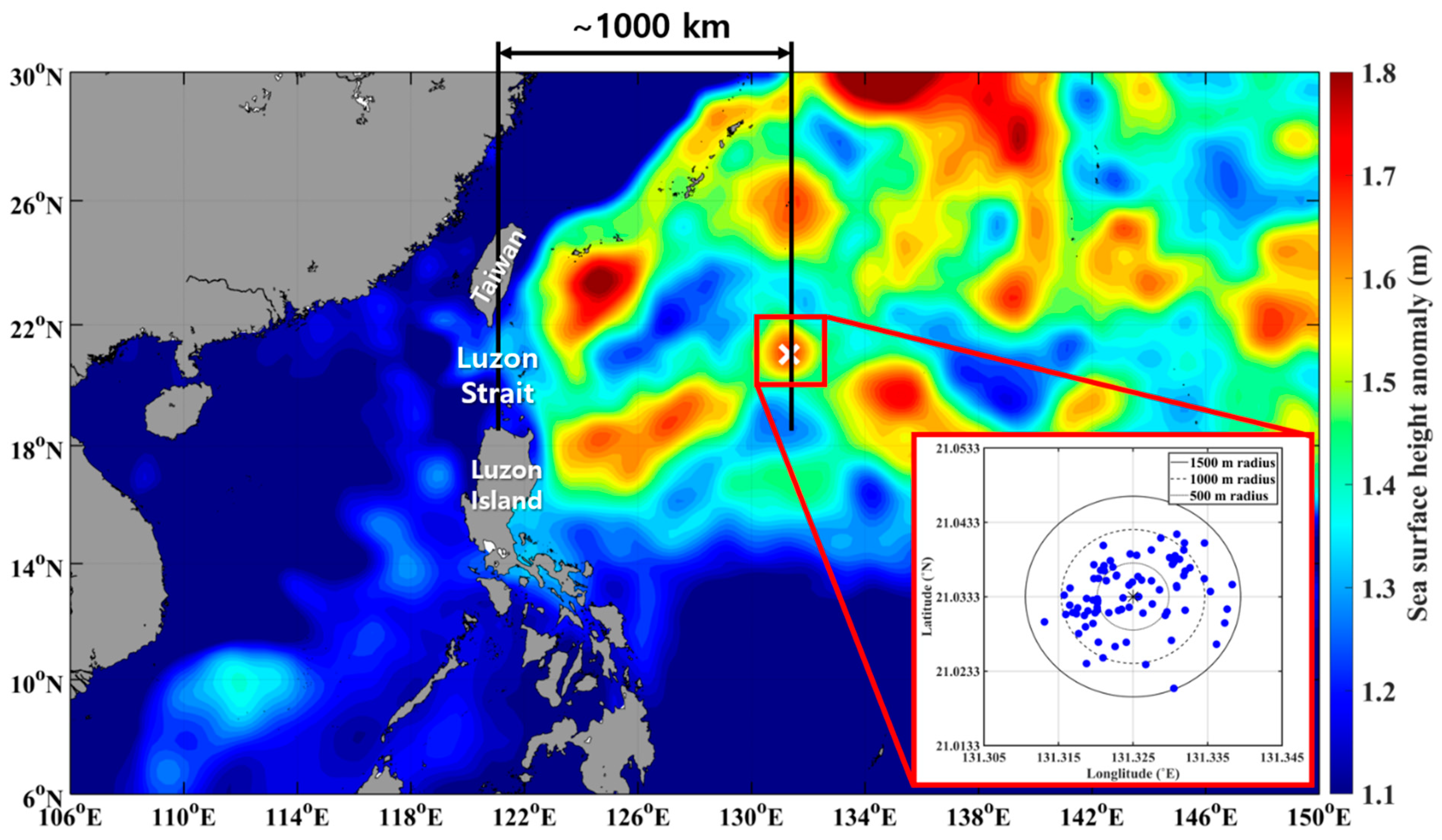
Figure 1.
A map of SSH (sea surface height) in the northwestern Pacific, including the study region marked by a white cross. The glider was carefully controlled on the surface within an RMS (root-mean square) of 720 m around the designated waypoint, as depicted in the inset.
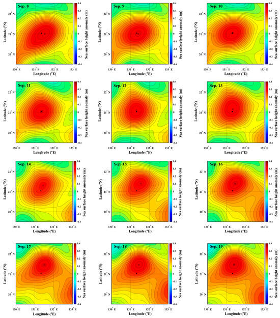
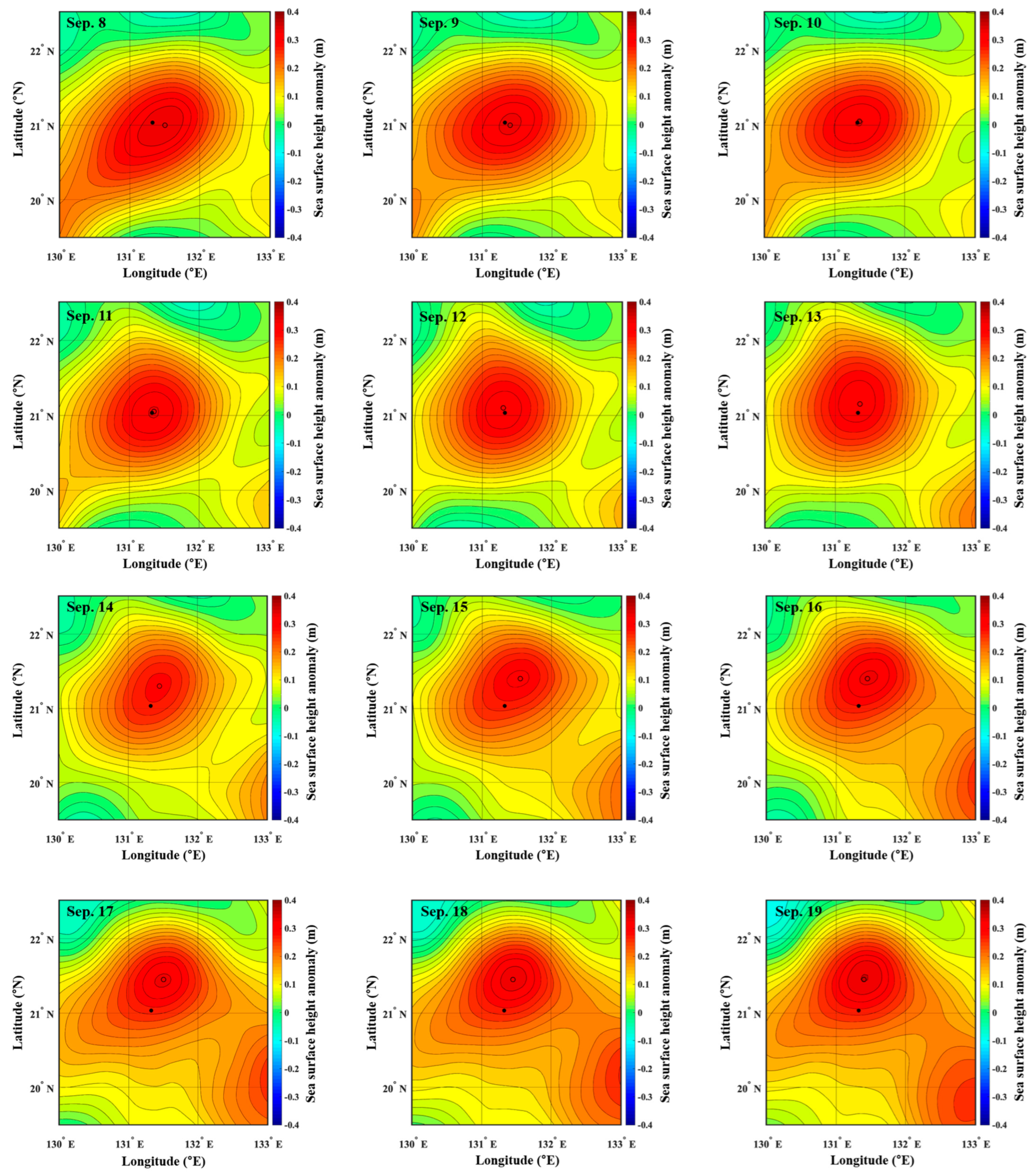
Figure 2.
Time evolution of SSHA (sea surface height anomaly) during observations in the study region, where a black dot denotes the glider’s virtual mooring (VM) location.
Wavelet analysis is a powerful technique for analyzing non-stationary signals or time series data with time-varying frequency content. There are several advantages over traditional power spectral analysis methods, such as the Fourier transform or periodogram. Firstly, it provides both time and frequency information [23], allowing for better localization of transient or non-stationary features in complex signals such as oceanic oscillatory phenomena. Secondly, it can capture features at different scales or resolutions, providing a more comprehensive understanding of the signal’s structure [24]. Thirdly, it can efficiently detect and characterize abrupt changes, discontinuities, or singularities in a signal [25]. Lastly, it can handle non-periodic or irregularly sampled signals, which are usually problematic for Fourier-based spectral analysis methods. These advantages make wavelet analysis particularly well-suited for analyzing complex, non-stationary, or noisy signals, such as those encountered in oceanic oscillatory phenomena.
Complex network theory can be applied to examine the structural variability of a complex system by representing the system as a network of interconnected nodes and edges. Nodes represent the components or elements of the system, and edges represent the interactions or relationships between them. By analyzing the network’s topology, structure, and dynamics, insights can be gained into the underlying mechanisms governing the complex system’s behavior [26]. There are several advantages to using complex network theory in this context. Firstly, it enables the simplification of complex systems into more manageable and understandable structures, revealing patterns, clusters, and interactions. Secondly, network metrics, such as degree distribution, clustering coefficient, and betweenness centrality, can provide quantitative descriptions of the system’s structural variability. Thirdly, the community detection algorithm [27,28] can reveal clusters or modules within the network, corresponding to functionally related components or subsystems within the system, and enhance understanding of the system’s organization and interactions. Lastly, it can be extended to study the time-varying structure of complex systems.
Based on the advantages of wavelet analysis and complex network methodology, we present a wavelet-coherence-based network methodology to analyze the structural variability of the internal waves system consisting of oscillatory multivariate time series with limited sample sizes and abrupt alterations or non-stationary behaviors. However, there are still potential pitfalls, such as threshold selection and the presence of noise or spurious correlations. We adopt statistical significance testing based on the ensemble of surrogate time series in order to avoid the spuriousness in pair-wise wavelet coherence estimation and arbitrariness in threshold selection. In this study, we make up 100 ensembles of the surrogate time series generated via the iAAWT (iterative amplitude-adjusted continuous wavelet transform) algorithm [29,30,31] and obtain critical values satisfying 95% significance level on pair-wise wavelet coherence estimates from those ensembles. If an estimated wavelet coherence is larger than its corresponding critical value, both time series are connected by an edge.
In this study, we examine the structural variations of internal tide systems, as an example of oscillatory systems, inside a mesoscale eddy, using our new approach based on a combination of wavelet analysis and complex network theory. The organization of this study is as follows. Section 2 contains the materials and methods. Analysis results are given in Section 3, and Section 4 presents the discussion.
2. Materials and Methods
2.1. Glider Measurements
The mission site, as illustrated in Figure 1, is situated amidst numerous warm (anticyclonic) and cold (cyclonic) eddies and is approximately 1000 km east of the Luzon Strait, which is an energetic source of internal tides and the primary passage between the Western Pacific (WP) and the South China Sea (SCS). In September 2018, a Slocum glider was deployed from the research vessel ISABU at 20.71° N and 131.11° E and actively navigated northeastward to a mesoscale warm eddy core at 21.03° N and 131.25° E, which was identified using Level 4 SSH satellite data from the Copernicus Marine Environmental Monitoring Service (CMEMS: https://marine.copernicus.eu/access-data, accessed on 8 September 2018). The glider was operated in virtual mooring (VM) mode by making a dive-and-climb from the surface to the depth of 800 m every 2.8 h, during which conductivity–temperature–depth (CTD) data were collected at a frequency of 4 Hz, providing a vertical resolution of approximately 0.5 m. Through the course of the glider measurement, the eddy slowly moved northward, allowing the glider to scan the spatial extent of the eddy from its core to periphery, corresponding to a distance of approximately 50 km (Figure 2).
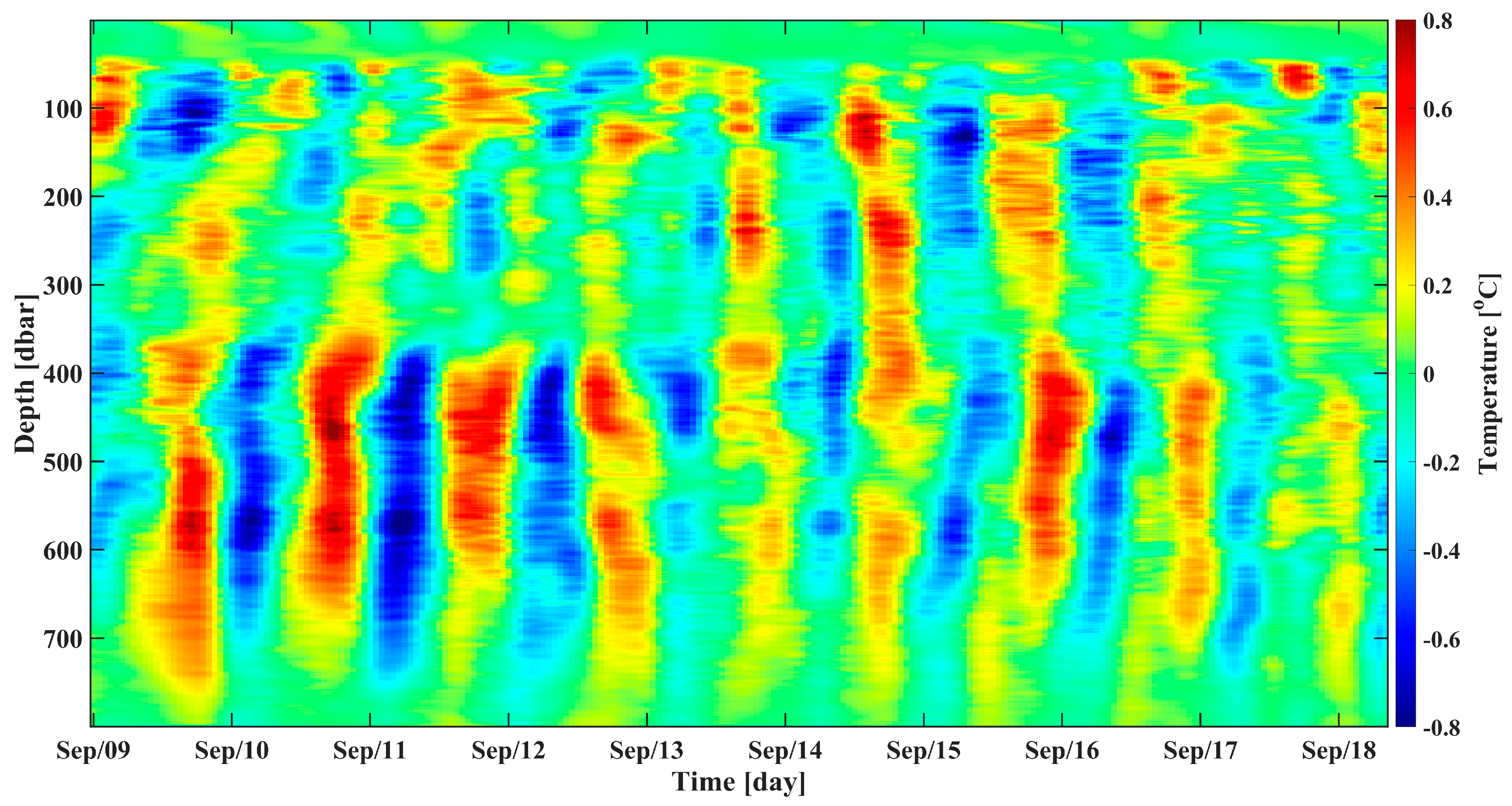
These in situ CTD measurements were interpolated and gridded to 1 m vertical and 1 h temporal resolution through a simple linear interpolation process. Further, a low-pass filter with a boxcar window of 10 m in the vertical direction and 5 h in the time direction was applied. To examine the variability of the internal wave system within the eddy, temperature anomalies that are closely related to internal wave behaviors were considered in this study. Temperature anomalies, defined as , were computed from the glider CTD data. Here, represents temperature time series, while is the background temperature obtained through averaging over the entire observation period. A time–depth map of the temperature anomalies with isotherms is displayed in Figure 3. For the following analysis, we reconstructed multivariate time series from the gridded data by selecting 25 depths separated by 30 m from the upper 50 m to the depth of 800 m. The top surface layer (below 50 m) was excluded owing to the uncertainty of glider measurements induced by the strong surface current, and the 30 m interval between successive depths was adopted in order to avoid spurious spatial correlations due to the gridding processing of raw measurement data.
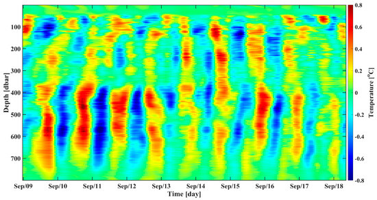
Figure 3.
A time–depth map of temperature anomalies, , obtained during the glider observation period within the anticyclonic eddy.
2.2. Wavelet Analysis Methodology
In this study, we use the Morlet wavelet, a complex continuous wavelet with zero mean, localized in both frequency and time [32]. The Morlet wavelet is defined as
where ω and τ represent the dimensionless frequency and time, respectively. With a dimensionless frequency of ω = 6, the Morlet wavelet provides an optimal balance between time and frequency localization, and its Fourier period, , is close to its scale () [33]. To extract features from a time series, , the continuous wavelet-transform (CWT) is applied as a convolution of with the scaled and normalized wavelet [34], expressed as
The wavelet power spectrum (WPS), , represents the power of the time series at each temporal period and its complex argument can be interpreted as the local phase. In order to find a dominant mode in a given time series, we use the global wavelet spectrum (GWS) as an analog of the Fourier transform spectrum, which is obtained by averaging the WPS estimates over the time duration [35], that is,
where denotes the time duration.
For evaluating the degree of correlation between two oscillating time series {, }, we compute the cross-wavelet transform (XWT), defined as , where denotes a complex conjugation [33,34]. Further, by normalizing the XWT, we define the wavelet coherence squared (WCS) of two time series [36], which is expressed as
where S is a smoothing operator [33]; the smoothing operator for the Morlet wavelet is given by Torrence and Webster [36]. The WCS indicates the coherence of XWT in time–frequency space and ranges from 0 to 1. In this work, a pair-wise WCS is used to construct a network from multivariate temperature anomaly time series through statistical significance testing based on surrogate data methods.
In order to perform statistical significance testing on WCS estimates through Monte Carlo methods, we construct 100 ensembles of the surrogate time series generated via the iAAWT algorithm, according to Schreiber and Schmitz [30], which consists of the following steps:
- Generation of a Gaussian white noise time series to match the length of the original data.
- Calculation of the continuous wavelet (Fourier) transform of the noise to extract its phase.
- Combination of the randomized phase and the wavelet transform modulus of the original signal to produce a surrogate time–frequency distribution.
- Reconstruction of a non-stationary surrogate time series by taking the real part of the inverse wavelet transform.
- Rescaling of the surrogate to match the distribution of the original time series.
The WCS estimates are calculated from each surrogate ensemble, and all the WCS ensembles at specific times and frequencies are used to obtain the corresponding critical value satisfying a 95% significance level; that is, one critical value is determined at every lattice point of time and frequency.
It is important to note that a wavelet analysis introduces an inherent limitation known as the cone of influence (COI) [32,33], referring to the region in which edge effects can influence the wavelet coefficients. In this study, we identified COI gaps for two specific scales: the semidiurnal and diurnal scales. These gaps are more or less the same within 1 day. Therefore, it should be noted that the reliable range of our wavelet-based analysis results spans from Day 2 to Day 8.
2.3. Network Construction
When constructing a WCS-based network, the critical values are used to determine whether WCS estimates are significant or not. If a WCS estimate is significant, that is, it is larger than its corresponding critical value, a pair of corresponding time series is connected by an edge. In this study, we constructed two kinds of WCS networks, each of which corresponds to a diurnal and semidiurnal period, respectively. Firstly, we computed a pair-wise WCS estimate matrix (, where is the number of periods, and denotes the sample size of a time series for a given pair of time series. Secondly, for specific diurnal and semidiurnal periods, we extracted a WCS row vector () of a specific period from the WCS matrix () and divided the WCS row vector into non-overlapping segments, with 24 h per segment. Thirdly, we averaged the WCS estimates belonging to each segment and assigned the mean WCS estimate to each segment. This mean WCS estimate was used to determine the connectivity for the corresponding pair of time series through comparison with the mean critical value of WCS. The critical value of WCS was computed from the WCS ensemble constructed via WCS computation (Equation (4)) performed on the 100 ensembles of surrogate times series following the iAAWT algorithm. Consequently, one network was constructed for every segment, and we obtained nine networks for the diurnal and semidiurnal periods (hereafter, DIT networks and SIT networks) because the sample size of our data was 225. This network construction procedure is schematically presented in Figure 4.
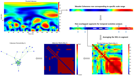
Figure 4.
Diagram of network construction procedure based on wavelet coherence squared (WCS).
2.4. Network Metrics
In this study, since we deal with time-varying and space-dependent modulations of internal tides, we focus on the connectivity among oscillations at different depths and the connectivity structure in terms of degrees [37], clustering coefficients [38], and community structures [27,28,39]. We also analyze the temporal evolution of the sum of minimal spanning tree (MST) weights in order to explore the variations in the overall connectivity and structure of a dynamic network over time [40,41]. Lastly, we examine the structural entropy quantifying the uncertainty or randomness in the organization of nodes across different communities or modules within the network [42].
The mean degree, defined as the average number of edges in the network, is obtained from the adjacency matrix {}, through [37]
where denotes the number of links attached to a node i and denotes mean degree of the network. Mean degree provides an idea of the overall connectivity of the network.
The clustering coefficient is a measure used to quantify the degree to which nodes in a network tend to cluster together or form tightly-knit groups. It describes the local structure and organization of the network by capturing the prevalence of triangles, i.e., sets of three interconnected nodes. The local and global clustering coefficients are defined as [38]
where denotes the number of real links among neighbors of a node i, and is the mean clustering coefficient.
The MST is a loop-less tree that spans all the nodes in a given network, such that the sum of the edge weights is minimized. For scale-dependent wavelet-coherence matrices, we compute corresponding distance matrices {} via the following formula [40]:
where denotes the averaged pair-wise WCS estimate of its corresponding matrix, and Kruskal’s algorithm is utilized to construct MST from the established distance matrix. In this study, the total weights of MST are used to examine the structural variability of a dynamic network.
Communities are groups of nodes that are densely connected to each other, with relatively fewer connections to nodes outside the group. Although there are some widely used algorithms, we adopt the Louvain algorithm based on modularity optimization [28]; this algorithm shows improvements in time consumption and optimization by using the improved modularity computation method and the network’s hierarchy structure. Modularity is a metric used in network analysis to evaluate the quality of a community structure [39], by measuring the difference between the actual number of edges within communities and the number of edges that would be expected by chance if the nodes were connected randomly while preserving the nodes’ degrees. Higher modularity values indicate that the network has a stronger community structure. The modularity metric, often denoted as Q, is defined as [39]
where is the total number of edges in the network, and are the degrees of nodes and , and are the community assignments of nodes and , and is the Kronecker delta function. Since, in this study, nodes represent depths, identified communities can provide information on vertical structural variabilities of DIT and SIT networks within a mesoscale eddy.
Structural entropy, in the context of network theory, is a measure quantifying the uncertainty or randomness in the organization of nodes across different communities or modules within the network. It can be used to analyze the complexity and diversity of community structures in any network and is calculated for a given community structure by applying Shannon entropy to the probability vector [42],
where is the size of community of a network with nodes. A high structural entropy value indicates a more diverse, complex, or disordered community structure, while a low value indicates a simpler or more homogeneous structure.
3. Analysis Results
3.1. Global Wavelet Spectra (WPS)
In this study, we use the GWS estimates (Equation (3)) to examine the power spectral characteristics of internal waves according to depths. To test the significance of the GWS estimates, we use 1000 surrogate time series generated via a simple AR-1 process as a red noise describing the oceanic background field [43], given by
where α represents the lag–1 autocorrelation of temperature anomaly series at each depth, and is taken from Gaussian white noise.
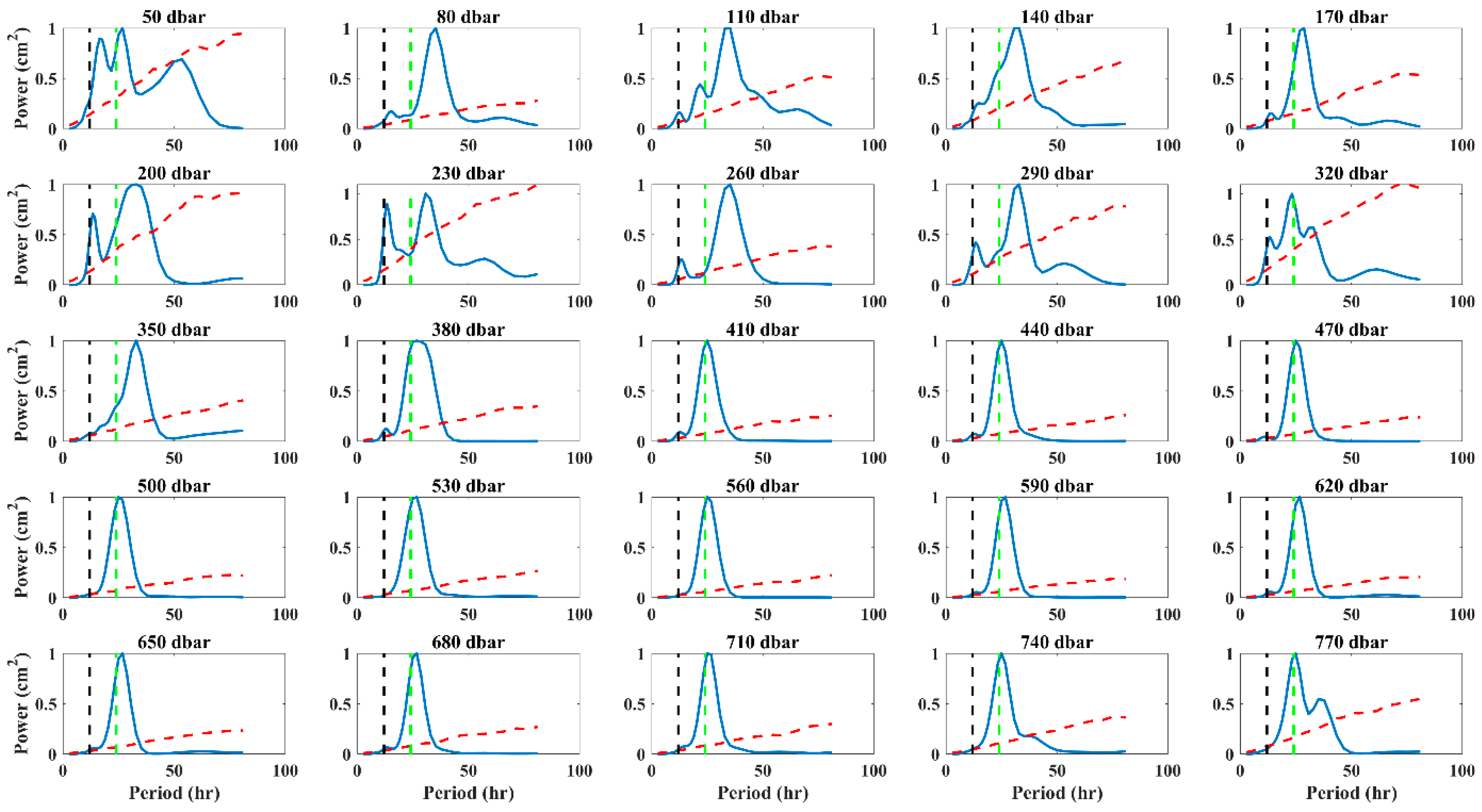
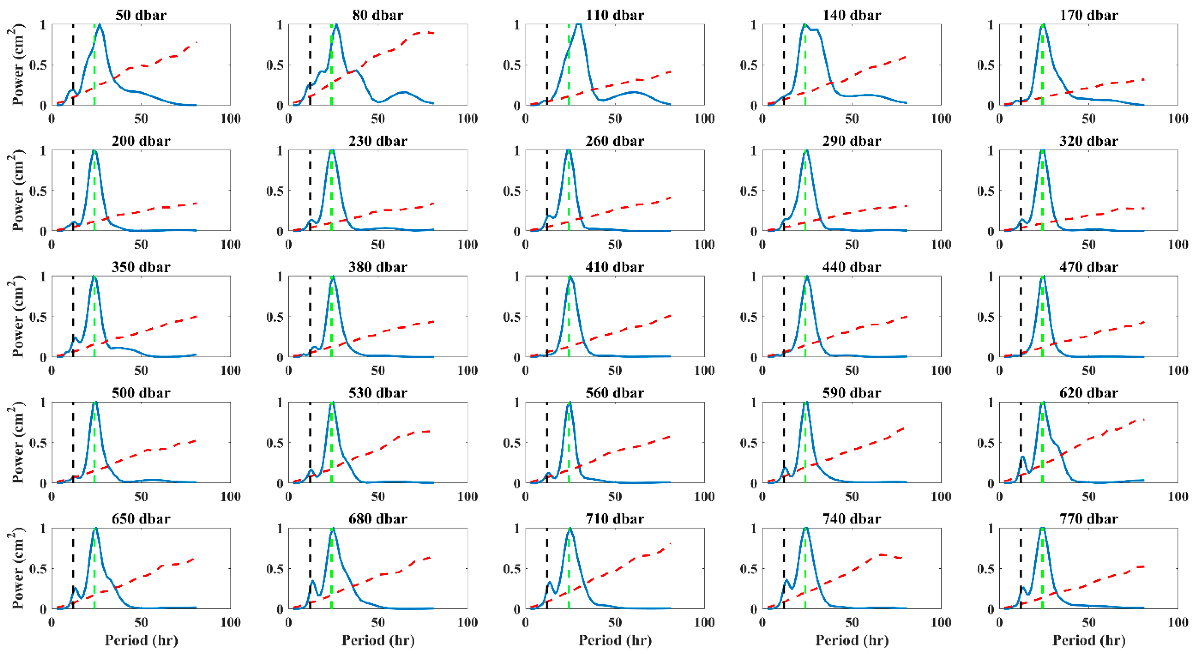
As shown in Figure 3, the oscillatory patterns of temperature anomalies seem to be distinct for two durations, the first duration (from 9/09 to 9/13) and the second duration (from 9/14 to 9/18). Thus, we compute GWS estimates separately for both periods and name them as the inner and outer centers of the eddy because the target eddy slowly migrated during the glider’s virtual mooring observations. The GWS estimates for both domains are presented in Figure 5 (inner center) and Figure 6 (outer center). The red dotted lines indicate the critical values satisfying a 95% significance level of the GWS distribution obtained from a surrogate ensemble consisting of 1000 time series generated via the AR1 process. All power estimates were scaled to the range of [0, 1] for comparison purposes by dividing by the maximum power value.
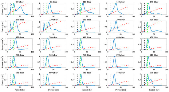
Figure 5.
The global wavelet spectra (GWS) estimates of temperature anomalies at 25 depths in the inner center. Black and green vertical dotted lines indicate the semidiurnal and diurnal periods, respectively.
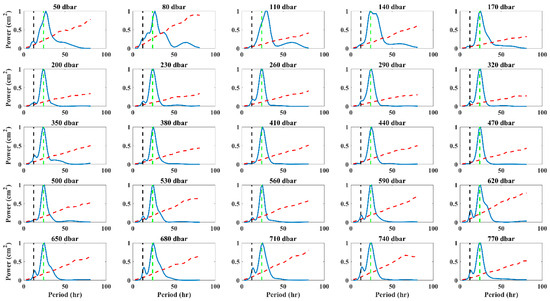
Figure 6.
Same as Figure 5 except for the outer center.
As shown in Figure 5 and Figure 6, the internal tides (DIT, diurnal internal tide; SIT, semidiurnal internal tide) are relatively dominant; the power of DITs is greater than that of SITs. The dominance of DIT over SIT is consistent with the fact that the study site is located approximately 1000 km eastward from the Luzon Strait, which is a representative generation site of internal tides. Further, Zhao [44] showed that the study site is significantly influenced by prevailing east-ward propagating DITs from the Luzon Strait.
Based on these observational facts, we construct wavelet-coherence networks corresponding to diurnal and semidiurnal periods in the following analysis. The difference in power spectral patterns between both domains (inner and outer centers) is clearly seen in the upper layer (above 400 m), while it greatly decreases in the lower layer (below 400 m), strongly indicating that the oceanic environments between the upper and lower layers are different. Also, the difference in power spectral patterns between the upper and lower layers is more dramatic in the inner center (Figure 5) than in the outer center (Figure 6), indicating that the oceanic environments between the inner and outer centers are different.
From these GWS analyses, we can identify two key observations regarding the structure and the influence of a mesoscale eddy on modulating internal tides. Firstly, a complex power spectral pattern is distinctly observed at depths between 50 and 320 dbar in the inner center (Figure 5), suggesting that the modulation of internal tides is actively taking place due to the significant impact of the investigated mesoscale eddy. In comparison to their behavior in the lower layer (below 400 dbar), the spatial extent of interactions between internal tides and the mesoscale eddy appears to be limited in the upper layer, indicating that the examined mesoscale eddy is primarily intensified near the surface. Secondly, the power spectral patterns observed in the outer center (Figure 6) are comparatively moderate when contrasted with those in the inner center, and they do not exhibit a significant difference between the upper and lower layers. This observation suggests that the mesoscale eddy’s influence on internal tide modulation is primarily concentrated in the upper layer of the inner center.
However, these spectral patterns do not provide insights into the phase variations of internal tides, which could reveal information about various interactions, such as the cascading processes of low modes into higher modes, harmonics, and subharmonics [7,11,12,13,15]. To address this, we employ the coherence-based network analysis focusing on the structural variations in phase and amplitude of the corresponding internal tides.
3.2. Internal Tides Networks
In the wavelet power spectra (Figure 5 and Figure 6), both diurnal internal tides (DIT) and semidiurnal internal tides (SIT) are found to be dominant. To investigate the dynamic aspects of internal tide modulation, we constructed daily-based networks corresponding to both internal tide periods, following the procedures outlined in the Network Construction section. We categorized the nodes into two subgroups representing the upper (circle) and lower (triangle) layers based on the results of wavelet spectral analysis. Then, using the Louvain algorithm, we examined the temporal evolution of network communities for both SIT and DIT networks.
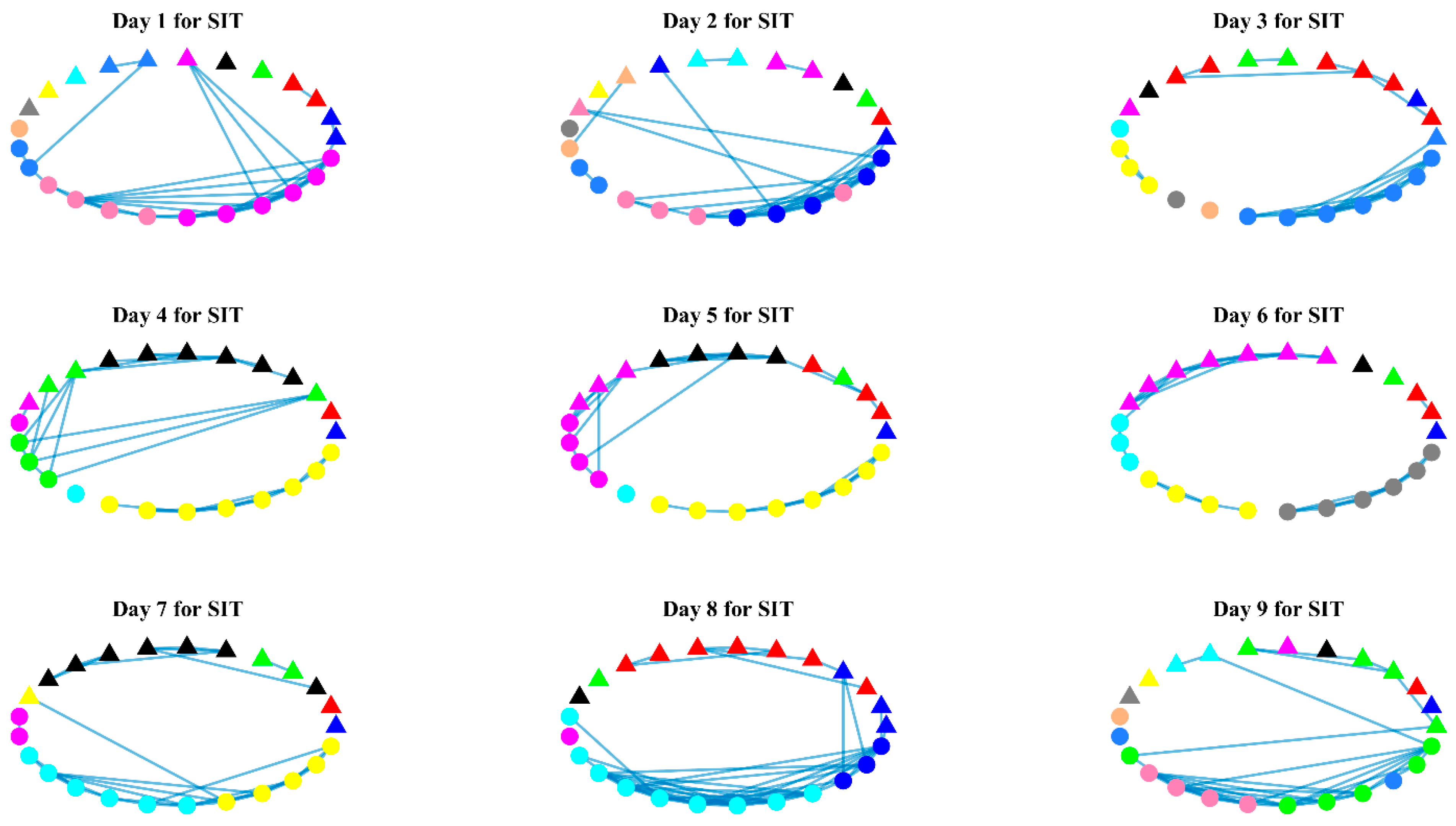
As illustrated in Figure 7, SIT networks exhibit two distinct characteristics: overall connectivity is low across all networks, and the modularity-based structure does not seem to vary significantly across both layers or over time. These observations indicate that SITs are incoherent among nodes, likely due to multiple SITs originating from external sources [44] and experiencing limited interactions within the eddy. If SITs were significantly interacting during the observation period, we would expect noticeable variability in different sub-domains. However, compared to DIT networks in Figure 8, there is no notable variation in network connectivity over time.
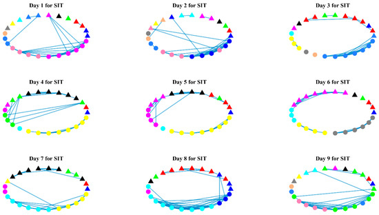
Figure 7.
SIT (Semidiurnal Internal Tide) networks. The colors denote the communities.
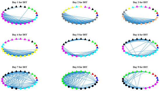
Figure 8.
Same as Figure 7 except for diurnal internal tide (DIT) networks.
Figure 8 reveals distinct behaviors in DIT networks compared to SIT networks (Figure 7). From Day 1 to Day 4, which represents the inner center, the lower layer (circle) displays a dense connectivity, while the upper layer (triangle) has a low connectivity. High connectivity signifies strong coherence among nodes, suggesting that the corresponding internal tides are not significantly modulated. Therefore, the considerably low connectivity in the upper layer indicates substantial modulation due to interactions between DITs and the mesoscale eddy.
From Day 6 onwards, the connectivity behavior changes dramatically, with increased interconnections between the upper and lower layers. This overall dense connectivity implies a noticeable reduction in the modulation of DITs. Additionally, the modularity-based community exhibits a distinct pattern—a clear separation between the upper and lower layers is visible in the inner center, while numerous communities emerge, linking nodes from both layers. In relation to the global wavelet spectra (GWS) behaviors depicted in Figure 5, these results demonstrate that internal tide modulations within the mesoscale eddy are primarily driven by interactions, such as subharmonics and cascading, between the diurnal internal tide (DIT) and the eddy. It is worth noting that our analysis findings are well consistent with the results of Lim and Park [45], in which a traditional vertical-mode decomposition method was used to reach the same conclusion.
3.3. Connectivity Characteristics of Networks
In this section, we characterize the dynamics of SIT and DIT networks in terms of connectivity (degree) and clustering coefficients (cliquishness). Further, in order to minimize the effect of low connectivity on the cliquishness of a network, we use the composite map of degrees and clustering coefficients. Also, to test the randomness of SIT and DIT networks, we used 100 ensembles of randomized networks (dotted line in Figure 9A), which are generated by randomizing the links of corresponding networks.
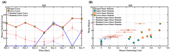
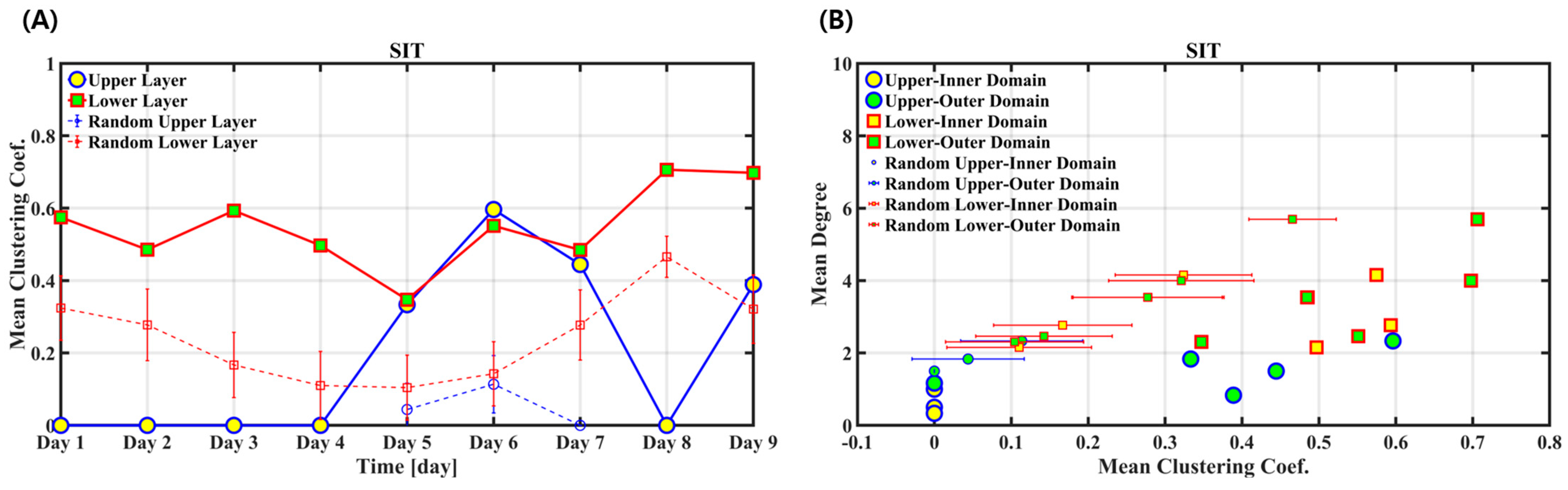
Figure 9.
A chart of mean clustering coefficients (A) and a composite map of mean degree and mean clustering coefficient (B) for SIT networks.
SIT networks show different behaviors in the upper and lower layers in terms of clustering coefficients, as shown in Figure 9. There is no difference between the inner and outer centers in the lower layer (Line with square in Figure 9A), while a dramatic change is observed in the upper layer (Line with circle in Figure 9A). However, caution should be taken in interpreting these behaviors in terms of interactions between SITs and the eddy, as the connectivity in the upper layer is too low. A clear observation is that there is little interaction in the lower layer (Figure 9A). From the composite map of the mean degree and mean clustering coefficients in Figure 9B, the lower layer seems to be irrespective of the horizontal domains (inner and outer centers; see color of square in Figure 9B), while the upper layer exhibits a clear differentiation between the inner and outer centers (except for one green node); the node, corresponding to Day 8 network, seems to be an abnormal behavior, probably due to sensitive incoherence feature of SITs [21].
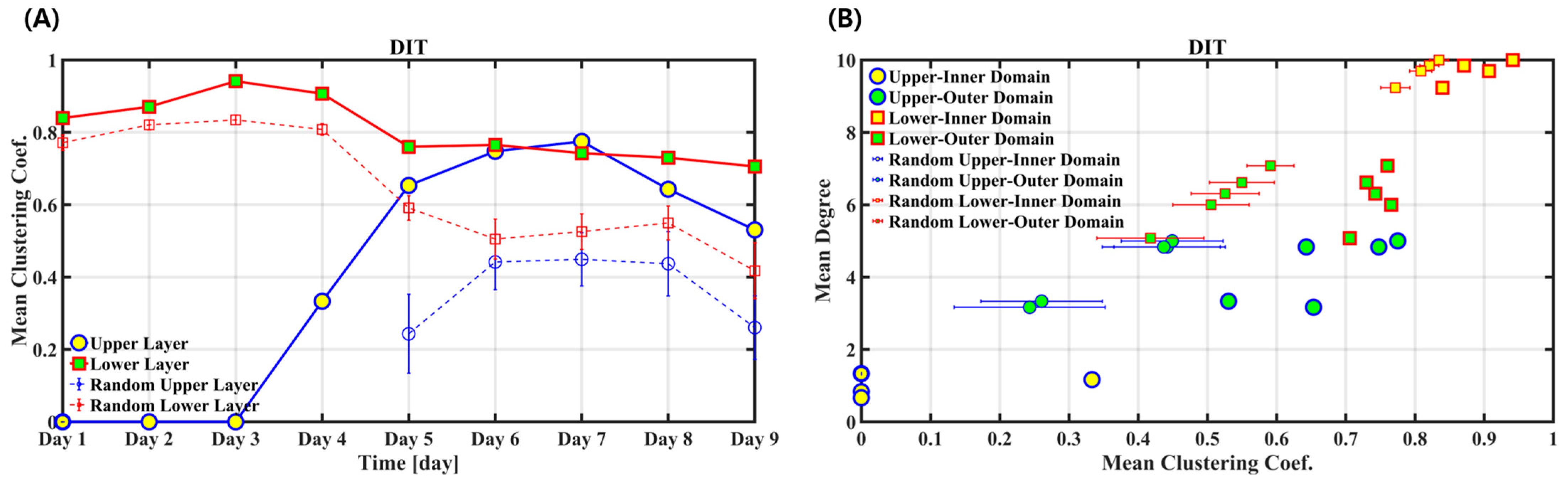
DIT networks show more clearly a differentiation between the inner and outer centers in the upper layer in terms of mean clustering coefficients (Figure 10A). Considering that DITs are the low-mode internal tides [4,5] originating solely from the Luzon strait [44], this behavior supports that there is a strong interaction between DITs and the eddy in the inner center. As in SIT networks, the mean clustering coefficients of DIT networks are irrespective of the horizontal domain in the lower layer. In the degree–clustering coefficient composite map (Figure 10B), there is a clear differentiation in the lower layer——a high degree and high clustering coefficient in the inner center compared to those in the outer center. This behavior can be due to a weakening effect of the interaction in the outer center, resulting in a loose cliquish structure in the lower layer due to strong inter-layer connectivity. In the upper layer (Circle in Figure 10B), a clear differentiation is observed; DIT networks in the outer center have a high mean degree and clustering coefficient, while they have low values in the inner center.
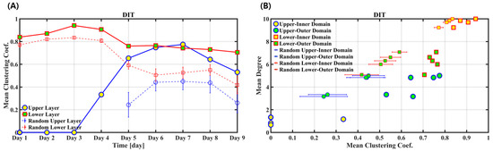
Figure 10.
Same as Figure 9 except for DIT (Diurnal Internal Tide) networks. A chart of mean clustering coefficients (A) and a composite map of mean degree and mean clustering coefficient (B) for DIT (Diurnal Internal Tide) networks.
Comparing the two network metrics, the clustering coefficient appears to be more reliable for assessing the structural variability of wavelet-coherence-based networks constructed from oscillatory time series. However, a composite approach with degree and clustering coefficients could be more appropriate.
3.4. Characteristics of Minimal Spanning Tree (MST)
To examine the variability of coherence structures of internal tides, we employ the total weights of MST networks to detect the distinguishing behavior in the sub-domains of the studied eddy. MST networks are established via Kruskal’s algorithm using distance matrices based on wavelet-coherence matrices for SIT and DIT signals, respectively. Thus, it should be noted that MST networks are different from the SIT and DIT networks because the MST networks are not subject to thresholding. The total weights of MST evaluate the degree of overall coherence of the wavelet-coherence matrix constructed from internal tides, with low values representing strong coherence and high values indicating incoherence. Since this value depends on the network’s size (number of nodes), we can make only qualitative evaluations via relative comparison.
For SITs, our analysis revealed that the lower layer is more coherent than the upper layer (Figure 11B,C), but the structural distinction between the inner (Day 1 through Day 5) and outer centers (Day 6 through Day 9) is not clear, as there is no distinctive variation pattern of MST weights between those horizontal domains.
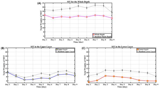
Figure 11.
The total weights of minimal spanning tree (MST): (A) for the whole depths (all nodes), (B) for the upper layer, and (C) for the lower layer.
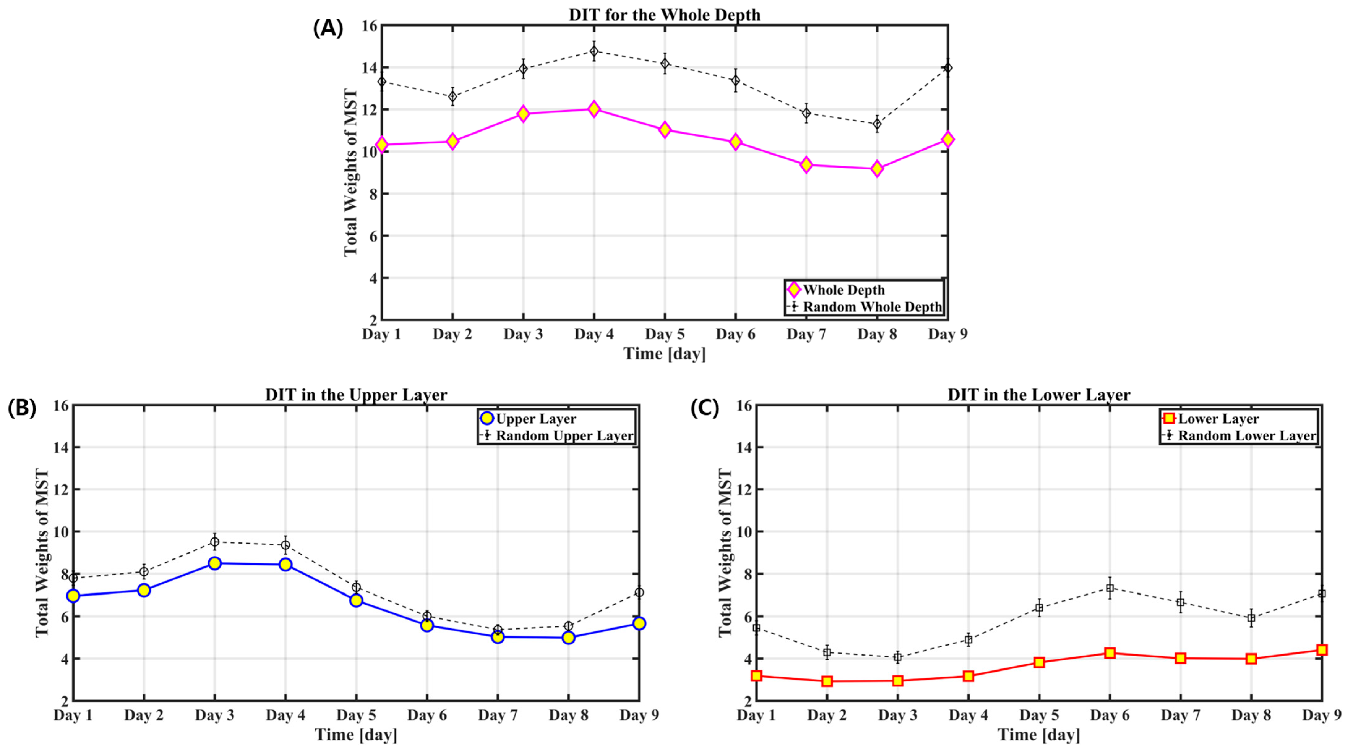
In contrast, for DITs, a distinct variability in MST weights in the upper layer is clearly observed (Figure 12B), with a high weight in the inner center and a low weight in the outer center, consistent with previous analysis results (Figure 10). It is important to note that all of these results are statistically significant compared to those of the wavelet-based surrogate dataset (see the dotted error bar in Figure 11 and Figure 12).
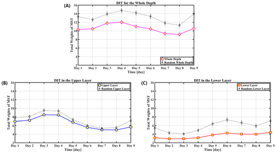
Figure 12.
Same as Figure 11 except for DIT minimal spanning trees (MSTs). The total weights of minimal spanning tree (MST): (A) for the whole depths (all nodes), (B) for the upper layer, and (C) for the lower layer.
It should be noted that the numerical values of MST weights for DITs are generally lower than those of SITs (as shown in Figure 11 and Figure 12); this difference could be caused by other factors rather than interactions. In Zhao’s study [44], it was found that SITs in the study area originated from multiple formation sites, while DITs mainly originated from the Luzon Strait. Therefore, it is important to take into consideration the multiplicity of internal tides in order to avoid spurious interactions when examining the modulation caused by interactions between internal tides and the eddy.
According to the definition of MST, low coherences among nodes result in a high MST total weight and vice versa. Thus, the overall exceeding trend of SIT over DIT, with no temporal trend (position-dependent pattern), implies that SIT’s incoherent behaviors are mainly due to the multiplicity of SITs at the study site rather than interactions between SITs and the eddy. If significant interactions existed between SITs and the eddy, a position-dependent pattern should be observed in the upper and lower layers, which is not the case (Figure 11). As for DITs, the pattern of total weights of MST in the upper layer is distinctive: the value is high in the inner center and low in the outer center (Figure 12B). These findings could be evidence of strong interactions between DITs and the eddy in the inner center of the upper layer and the horizontal inhomogeneity of a surface-intensified mesoscale eddy.
3.5. Structural Variability of Networks
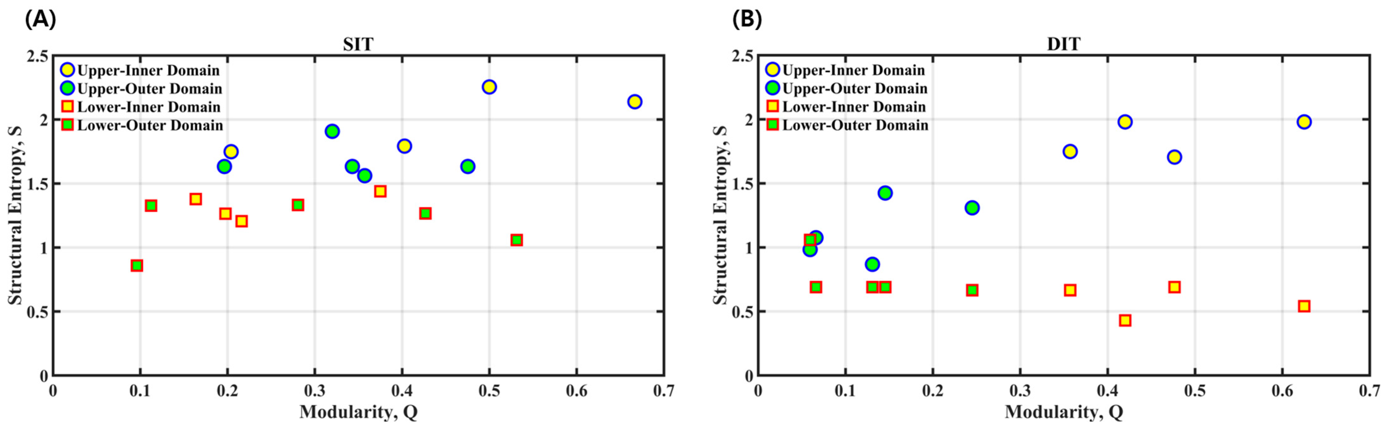
To investigate the variability in the structure of internal tide networks, we utilized the concept of structural entropy [42], which is based on the community structure within a network. The connection between modularity and structural entropy is presented in Figure 13; a high level of modularity signifies a robust community structure within a network. For SIT networks (Figure 13A), there is no discernible pattern in either structural entropy or modularity for horizontal domains (inner and outer centers). However, for vertical domains (upper and lower layers), a clear differentiation in structural entropy is evident. A little difference in structural entropy for both layers suggests that SITs are weakly influenced by the surface-intensified mesoscale eddy in the upper layer.
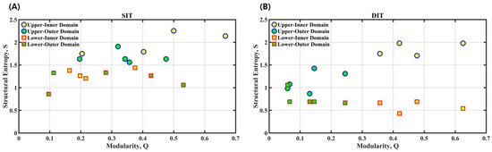
Figure 13.
A composite map of structural entropy and modularity for SIT networks (A) and DIT networks (B).
Contrary to SIT networks, DIT networks exhibit distinct patterns in both structural entropy and modularity (Figure 13B): (1) they display high modularity in the inner center and low modularity in the outer center, (2) the upper layer exhibits a higher structural entropy compared to the lower layer, and (3) there is a significant contrast in structural entropy within the inner center for both layers. These findings appear to clarify two aspects: (1) DITs are profoundly influenced by the eddy in the inner center of the upper layer, and (2) DITs exhibit sensitivity to their position within a mesoscale eddy (indicated by colored circles in Figure 13B).
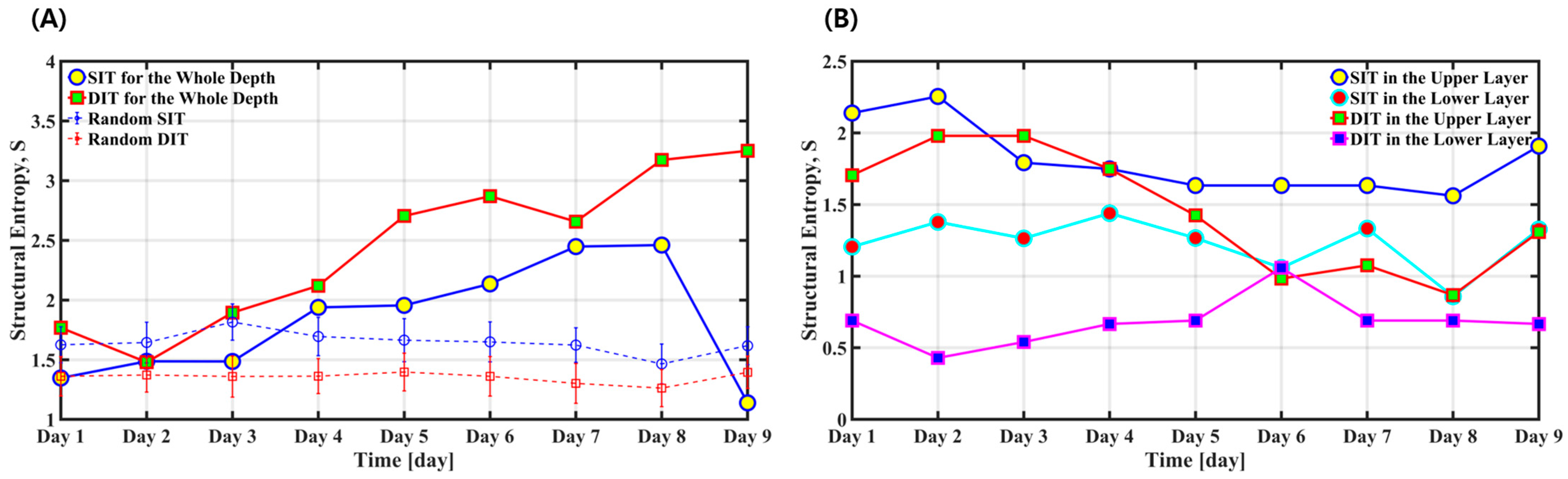
Time in our data corresponds to the horizontal position within a mesoscale eddy (Figure 2) as the eddy slowly migrates during the glider’s virtual mooring observations. Therefore, we examine the temporal evolution of the structural entropy of internal tide networks to understand the structural variability of these networks. The whole-depth networks of both SIT and DIT (Figure 14A) exhibit a growing trend (with the exception of Day 9 in SIT networks), suggesting that the community structure within both networks becomes more random in the outer center compared to the inner center. This behavior is well contrasted with our previous findings, where DITs seem to be more influenced by the eddy in the inner center than in the outer center. This result implies that the concept of structural entropy should be employed with caution; as stated in Almog and Shmueli [42], social networks based on certain social factors and brain networks based on anatomy could be inappropriate for this approach. The full-depth SIT and DIT networks seem to belong to those networks from the perspective of geometricity, similar to anatomy in the brain system.
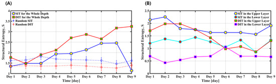
Figure 14.
Temporal evolution of structural entropy for SIT networks and DIT networks. (A) Temporal evolutions of structural entropy of SIT and DIT networks for the whole depth, with those of randomized SIT and DIT networks. (B) Temporal evolutions of structural entropy of SIT and DIT networks for repsective sub-layer.
When we apply the structural entropy methodology separately to the upper and lower layers (Figure 14B), the structural entropy is noticeably high in the upper layer. This indicates that the upper layer is influenced by the surface-intensified eddy. Moreover, for DIT networks, the horizontal domains are clearly distinguished, implying that DITs in the inner center are strongly modulated by the eddy compared to those in the outer center (green square in Figure 14B). This position-dependent behavior of DITs within the eddy is consistent with the results of our previous analyses.
4. Discussion
In this study, we introduced a wavelet-coherence-based network methodology to examine the modulation of internal tides within a mesoscale anticyclonic eddy. Our glider dataset has a spatiotemporal limitation; its spatial coverage is very limited to the upper surface layer (up to 800 m depth) compared to the full depth of 6000 m, and its temporal span is less than 10 days (225 h). Due to these restrictions, the previous analysis by Lim and Park [45] required additional datasets, such as ADCP from the research vessel ISABU and satellite-based measurements. However, our new approach has an advantage in obtaining the same results solely from the glider’s observations.
By exploiting a wavelet approach optimized for the time–frequency locality, we found the spatial dependency of modulations of internal tides inside the mesoscale anticyclonic eddy, strongly indicating that the eddy is intensified in the surface layer (less than 400 m) and exhibits a varying strength of interaction depending on the distance from the eddy’s center point; as reported in Lim and Park [45], interactions are more actively occurring in the inner center (within 30 km of the eddy’s center point) due to its high relative vorticity.
The distinct behaviors of SIT and DIT networks within the mesoscale eddy, in terms of network metrics, such as mean degree and mean clustering coefficients, are consistent with observational and numerical facts [7,45] that the horizontal scale of the eddy is comparable to that of the lowest mode of DIT. This distinction is also confirmed by the total weights of MST and modularity-based structural entropy. Consequently, the interactions between internal tides and mesoscale eddies are scale- and position-dependent in the interior of the eddy. Since a mesoscale eddy changes the nearby current velocity and density (temperature and salinity) [22], it is important to know the interaction level of internal tides and mesoscale eddies in terms of spatial scale and position. To this end, further empirical studies should be conducted.
The methodology introduced in this study successfully detected the spatial characteristics of a mesoscale anticyclonic eddy in real oceanic environments through network metrics, employing a spatiotemporally limited dataset such as glider measurements. However, this methodology is too limited and has some challenges in its applicability. Also, we should validate the methodology through various empirical studies for its extensive applicability. In the next study, we will verify the validity by applying this method and its variants to other oscillatory systems.
Author Contributions
Conceptualization, G.L. and J.-J.P.; methodology, G.L.; validation, G.L. and J.-J.P.; formal analysis, G.L. and J.-J.P.; investigation, G.L. and J.-J.P.; data curation, J.-J.P.; writing—original draft preparation, G.L.; writing—review and editing, J.-J.P.; visualization, G.L. and J.-J.P.; supervision, J.-J.P.; project administration, J.-J.P.; funding acquisition, J.-J.P. All authors have read and agreed to the published version of the manuscript.
Funding
This research was supported by the Korea Institute of Marine Science & Technology Promotion (KIMST) funded by the Ministry of Oceans and Fisheries (RS-2020-KS201379, RS-2023-00256005).
Data Availability Statement
The data presented in this study are available upon request from the corresponding author.
Acknowledgments
This study has been conducted using E.U. Copernicus Marine Service Information; https://doi.org/10.48670/moi-00145, accessed on 1 December 2023.
Conflicts of Interest
The authors declare no conflicts of interest.
References
- Munk, W.; Wunsch, C. Abyssal recipes II: Energetics of tidal and wind mixing. Deep. Sea Res. Part I 1998, 45, 1977–2010. [Google Scholar] [CrossRef]
- Wunsch, C.; Ferrari, R. Vertical mixing, energy, and the general circulation of the oceans. Annu. Rev. Fluid Mech. 2004, 36, 281–314. [Google Scholar] [CrossRef]
- Löb, J.; Köhler, J.; Mertens, C.; Walter, M.; Li, Z.; von Storch, J.S.; Zhao, Z.; Rhein, M. Observations of the low-mode internal tide and its interaction with mesoscale flow south of the Azores. J. Geophys. Res. 2020, 125, e2019JC015879. [Google Scholar] [CrossRef]
- Alford, M.H. Redistribution of energy available for ocean mixing by long-range propagation of internal waves. Nature 2003, 423, 159–162. [Google Scholar] [CrossRef]
- Tian, J.; Zhou, L.; Zhang, X.; Liang, X.; Zheng, Q.; Zhao, W. Estimates of M2 internal tide energy fluxes along the margin of northwestern pacific using TOPEX/POSEIDON altimeter data. Geophys. Res. Lett. 2003, 30, 1889. [Google Scholar] [CrossRef]
- Arbic, B.K. Incorporating tides and internal gravity waves within global ocean general circulation models: A review. Prog. Oceanogr. 2022, 206, 102824. [Google Scholar] [CrossRef]
- Dunphy, M.; Lamb, K.G. Focusing and vertical mode scattering of the first mode internal tide by mesoscale eddy interaction. J. Geophys. Res. Ocean 2014, 119, 523–536. [Google Scholar] [CrossRef]
- Huang, X.; Zhang, Z.; Zhang, X.; Qian, H.; Zhao, W.; Tian, J. Impacts of a mesoscale eddy pair on internal solitary waves in the northern south China Sea revealed by mooring array observations. J. Phys. Oceanogr. 2017, 47, 1539–1554. [Google Scholar] [CrossRef]
- Huang, X.; Wang, Z.; Zhang, Z.; Yang, Y.; Zhou, C.; Yang, Q.; Zhao, W.; Tian, J. Role of mesoscale eddies in modulating the semidiurnal internal tide: Observation results in the northern south China Sea. J. Phys. Oceanogr. 2018, 48, 1749–1770. [Google Scholar] [CrossRef]
- Whalen, C.B.; De Lavergne, C.; Naveira Garabato, A.C.; Klymak, J.M.; MacKinnon, J.A.; Sheen, K.L. Internal wave-driven mixing: Governing processes and consequences for climate. Nat. Rev. Earth Environ. 2020, 1, 606–621. [Google Scholar] [CrossRef]
- Lelong, M.-P.; Riley, J.J. Internal wave-vortical mode interactions in strongly stratified flows. J. Fluid Mech. 1991, 232, 1–19. [Google Scholar] [CrossRef]
- McComas, C.H.; Bretherton, F.P. Resonant interaction of oceanic internal waves. J. Geophys. Res. 1977, 82, 1397–1412. [Google Scholar] [CrossRef]
- Bartello, P. Geostrophic adjustment and inverse cascades in rotating stratified turbulence. J. Atmos. Sci. 1995, 52, 4410–4428. [Google Scholar] [CrossRef]
- Bühler, O.; Mclntyre, M.E. Wave capture and wave-vortex duality. J. Fluid Mech. 2005, 534, 67–95. [Google Scholar] [CrossRef]
- Chavanne, C.; Flament, P.; Luther, D.; Gurgel, K.-W. The surface expression of semidiurnal internal tides near a strong source at Hawaii: Part II: Interactions with mesoscale currents. J. Phys. Oceanogr. 2010, 40, 1180–1200. [Google Scholar] [CrossRef]
- Kerry, C.G.; Powell, B.S.; Carter, G.S. The impact of subtidal circulation on internal tide generation and propagation in the Philippine Sea. J. Phys. Oceanogr. 2014, 44, 1386–1405. [Google Scholar] [CrossRef]
- Guo, Z.; Wang, S.; Cao, A.; Xie, J.; Song, J.; Guo, X. Refraction of the M2 internal tides by mesoscale eddies in the South China Sea. Deep-Sea Res. I. 2023, 192, 103946. [Google Scholar] [CrossRef]
- Whalen, C.B.; Talley, L.D.; MacKinnon, J.A. Spatial and temporal variability of global ocean mixing inferred from argo profiles. Geophys. Res. Lett. 2012, 39, L18612. [Google Scholar] [CrossRef]
- Song, P.; Chen, X. Investigation of the internal tides in the Northwest Pacific Ocean considering the background circulation and stratification. J. Phys. Oceanogr. 2020, 50, 3165–3188. [Google Scholar] [CrossRef]
- Li, B.; Du, L.; Peng, S.; Yuan, Y.; Meng, X.; Lv, X. Modulation of Internal Tides by Turbulent Mixing in the South China Sea. Front. Mar. Sci. 2021, 8, 772979. [Google Scholar] [CrossRef]
- Li, B.; Wei, Z.; Wang, X.; Fu, Y.; Fu, Q.; Li, J.; Lv, X. Variability of coherent and incoherent features of internal tides in the north South China Sea. Sci. Rep. 2020, 10, 12904. [Google Scholar] [CrossRef]
- Wang, P.; Mao, K.; Chen, X.; Liu, K. The three-dimensional structure of the mesoscale eddy in the Kuroshio Extension region obtained from three datasets. J. Mar. Sci. Eng. 2022, 10, 1754. [Google Scholar] [CrossRef]
- Meyers, S.D.; Kelly, B.G.; O’Brien, J.J. An introduction to wavelet analysis in oceanography and meteorology: With application to the dispersion of Yanai waves. Mon. Weather Rev. 1993, 121, 2858–2866. [Google Scholar] [CrossRef]
- Rhif, M.; Ben Abbes, A.; Farah, I.R.; Martínez, B.; Sang, Y. Wavelet Transform Application for/in Non-Stationary Time-Series Analysis: A Review. Appl. Sci. 2019, 9, 1345. [Google Scholar] [CrossRef]
- Pothisarn, C.; Klomjit, J.; Ngaopitakkul, A.; Jettanasen, C.; Asfani, D.A.; Negara, I.M.Y. Comparison of Various Mother Wavelets for Fault Classification in Electrical Systems. Appl. Sci. 2020, 10, 1203. [Google Scholar] [CrossRef]
- Newman, M.E.J. The Structure and Function of Complex Networks. SIAM Rev. 2003, 45, 167–256. Available online: http://www.jstor.org/stable/25054401 (accessed on 22 January 2024). [CrossRef]
- Newman, M.E.J. Modularity and community structure in networks. Proc. Natl. Acad. Sci. USA 2006, 103, 8577–8582. [Google Scholar] [CrossRef]
- Blondel, V.D.; Guillaume, J.L.; Lambiotte, R.; Lefebvre, E. Fast unfolding of communities in large networks. J. Stat. Mech. 2008, 2008, 10008. [Google Scholar] [CrossRef]
- Theiler, J.; Eubank, S.; Longtin, A.; Galdrikian, B.; Farmer, J.D. Testing for nonlinearity in time series: The method of surrogate data. Phys. D Nonlinear Phenom. 1992, 58, 77–94. [Google Scholar] [CrossRef]
- Schreiber, T.; Schmitz, A. Surrogate time series. Phys. D Nonlinear Phenom. 2000, 142, 346–382. [Google Scholar] [CrossRef]
- Chavez, M.; Cazelles, B. Detecting dynamic spatial correlation patterns with generalized wavelet coherence and non-stationary surrogate data. Sci. Rep. 2019, 9, 7389. [Google Scholar] [CrossRef]
- Farge, M. Wavelet transforms and their applications to turbulence. Annu. Rev. Fluid Mech. 1992, 24, 395–457. [Google Scholar] [CrossRef]
- Torrence, C.; Compo, G. A practical guide to wavelet analysis. Bull. Am. Meteorol. Soc. 1998, 79, 61–78. [Google Scholar] [CrossRef]
- Grinsted, A.; Moore, J.C.; Jevrejeva, S. Application of the cross wavelet transform and wavelet coherence to geophysical time series. Nonlin. Process. Geophys. 2004, 11, 561–566. [Google Scholar] [CrossRef]
- Wu, S.; Liu, Q. Some problems on the global wavelet spectrum. J. Ocean Univ. China 2005, 4, 398–402. [Google Scholar] [CrossRef]
- Torrence, C.; Webster, P.J. The annual cycle of persistence in the El Niño/Southern Oscillation. Q. J. R. Meteorol. Soc. 1998, 124, 1985–2004. [Google Scholar] [CrossRef]
- Boccaletti, S.; Latora, V.; Moreno, Y.; Chavez, M.; Hwang, D.U. Complex networks: Structure and dynamics. Phys. Rep. 2006, 424, 175–308. [Google Scholar] [CrossRef]
- Watts, D.J.; Strogatz, S.H. Collective dynamics of ‘small-world’ networks. Nature 1998, 393, 440–442. [Google Scholar] [CrossRef]
- Newman, M.E.J.; Girvan, M. Finding and evaluating community structure in networks. Phys. Rev. E 2004, 69, 026113. [Google Scholar] [CrossRef]
- Mantegna, R.N. Hierarchical structure in financial markets. Eur. Phys. J. B 1999, 11, 193–197. [Google Scholar] [CrossRef]
- Wang, G.J.; Xie, C.; Chen, S. Multiscale correlation networks analysis of the US stock market: A wavelet analysis. J. Econ. Interact. Coord. 2017, 12, 561–594. [Google Scholar] [CrossRef]
- Almog, A.; Shmueli, E. Structural Entropy: Monitoring Correlation-Based Networks Over Time with Application to Financial Markets. Sci. Rep. 2019, 9, 10832. [Google Scholar] [CrossRef] [PubMed]
- Labat, D. Oscillations in land surface hydrological cycle. Earth Planet. Sci. Lett. 2006, 242, 143–154. [Google Scholar] [CrossRef]
- Zhao, Z. Internal tide radiation from the Luzon strait. J. Geophys. Res. 2014, 119, 5434–5448. [Google Scholar] [CrossRef]
- Lim, G.; Park, J.J. Vertical structural variability of diurnal internal tides inside a mesoscale anticyclonic eddy based on single virtual-moored Slocum glider observations. Front. Mar. Sci. 2022, 9, 920049. [Google Scholar] [CrossRef]


Disclaimer/Publisher’s Note: The statements, opinions and data contained in all publications are solely those of the individual author(s) and contributor(s) and not of MDPI and/or the editor(s). MDPI and/or the editor(s) disclaim responsibility for any injury to people or property resulting from any ideas, methods, instructions or products referred to in the content. |
© 2024 by the authors. Licensee MDPI, Basel, Switzerland. This article is an open access article distributed under the terms and conditions of the Creative Commons Attribution (CC BY) license (https://creativecommons.org/licenses/by/4.0/).