Abstract
The position of the laminar–turbulent flow transition affects the aerodynamic efficiency of wind turbine rotor blades. An established diagnostic tool is infrared thermography, which enables flow visualization on in-service wind turbines, including the detection of the flow transition position. For the first time, the capabilities of a Bayesian-based image evaluation on the basis of previous knowledge are investigated for maximizing the measurement quality in particular for those weather conditions with a low contrast-to-noise ratio. The Bayesian framework is assessed using simulated and measured thermographic images, incorporating a probability distribution of the transition position. Results indicate that utilizing previous knowledge, especially when normally distributed around the true transition position with a standard deviation of px, significantly reduces uncertainty for thermographic images with a contrast-to-noise ratio . Additionally, the Bayesian framework enhances the visualization of transition progression along the radial blade axis, yielding a less noisy result. Previous experimental data can be used to reduce uncertainty for erroneous transition position detections. In conclusion, the integration of high-quality previous knowledge through Bayesian inference proves to be effective in lowering the uncertainty of the position measurement of the laminar–turbulent transition on wind turbine rotor blades, with no compromise of the spatiotemporal resolution.
1. Introduction
1.1. Motivation
The demand for renewable energy has increased significantly over the past few years due to the growing concern for the climate and the need for sustainable energy sources. Wind turbines are a popular source of renewable energy, but their efficiency is affected by the boundary layer flow conditions, particularly the laminar–turbulent transition. The position of the transition is an important factor for the performance of the turbine. Any defects or contamination on the surface of the rotor blades introduce turbulence that shifts the transition away from the designed position and results in a lower aerodynamic efficiency [1]. Therefore, in order to understand the real flow behavior and, subsequently, to optimize the aerodynamic performance, it is crucial to measure the position of the laminar–turbulent flow transition on the rotor blade in-process, i.e., on an operating wind turbine.
1.2. State of the Art
A measurement method to analyze the laminar–turbulent flow transition on wind turbines is the use of pressure sensors [2]. Pressure sensors have successfully been applied on wind turbines, but the time-consuming installation of these sensors leads to long downtimes of the wind turbine. Doppler Global Velocimetry (DGV) [3,4] and Particle Image Velocimetry (PIV) [5] are known non-invasive, direct flow field measuring techniques. However, both measurement principles have severe limitations for ground-based boundary layer flow measurements on the rotor blades of operating wind turbines. The large measuring distance (> m), the large size of the wind turbine rotor and the large volume of airflow involved result in low contrast-to-noise ratios (CNR) and low spatial resolutions. Both limitations make these methods less suitable for in-process measurements on wind turbines.
As an alternative, infrared thermography (IRT) is an optical flow visualization method that relies on the different heat transfer in the different boundary layer flow regimes. It provides fast, non-invasive flow imaging from large distances. In wind tunnel experiments, the capability of IRT to visualize the laminar–turbulent transition [6], laminar separation bubbles [7] or turbulent separation [8] was proven. However, the exposure time for one camera image is limited to cope with the motion blur of the moving rotor blade. Gazzini et al. addressed the challenges of motion blur and camera noise by employing two integration times. They effectively combined 16,000 images of a turbine rotor blade using a filtering and de-blurring process [9]. Von Hoesslin et al. employed temperature decline thermography to visualize the boundary layer state on a turbine rotor with reduced noise [10].
IRT has further been demonstrated as a convenient method for determining the laminar–turbulent transition on rotor blades [11]. The laminar–turbulent transition is determined by evaluating the intensity of the thermograms, and Dollinger et al. [12] and Reichstein et al. [13] were the first to apply this method for in-process measurements on wind turbines.
Using IRT on wind turbines, the CNR of the thermographic images is limited due to the field conditions (for instance low solar radiation) or a small sensitivity of the measurement effect (as seen in the detection of static [14] or dynamic stall [15], or when using small-signal evaluation approaches such as differential images tested on an airfoil [16] and rotor blades of wind turbines [17]). Gleichauf et al. improved the contrast with averaging methods, i.e., non negative Matrix factorization [18] and principle component analysis [19]. Nevertheless, without including previous knowledge, the available CNR directly limits the achievable measurement uncertainty for the determination of the laminar–turbulent transition position on the rotor blade of a wind turbine. However, even though every rotor blade is different and suffers different conditions over its lifespan, they also share many common characteristics and, presumably, behave similarly in the wind. Therefore, it needs to be investigated whether previous knowledge, which means information that has been gained on previous experiments or simulations, can improve the IRT-based measurement of the laminar–turbulent transition position on wind turbine rotor blades.
Since such an investigation is missing for the IRT-based flow visualization, understanding how to include previous knowledge into a measurement means reaching out to other fields of research. Mohammady and Miyadera used previous knowledge in the form of a physical law as a constraint to improve their measurement [20]. Constraints are a straightforward approach to including previous knowledge, but previous knowledge cannot always be formulated in a suitable form. A more general way is to think of previous knowledge in the form of a probability distribution for the transition to be at a certain position. The framework to update prior beliefs in the form of probability functions with additional information from experimental data is known as the Bayesian inference, which was found by Thomas Bayes and published posthumously by Richard Price in 1763 [21]. The discovery of Markov chain Monte Carlo methods, usually credited to Gelfand et al. [22], led to a dramatic growth in research and applications of Bayesian methods. Meija et al. provide an overview of how the Bayesian analysis has been adapted to many different research problems in metrology [23]; Kruschke says: “The 21st century is becoming Bayesian” [24]. Frequent statistics, which are an alternative to the Bayesian analysis, are compared by Attivissimo et al., concluding that both approaches are generally applicable in metrology [25]. However, the Bayesian approach is considered to fit better because the definition of the previous knowledge as a random variable with a probability distribution is feasible for the use case, and it provides an implicit uncertainty evaluation in accordance with the GUM [26].
Even though Bayesian inference is commonly accepted as the standard for combining previous knowledge with measurement data, its applicability for the thermographic flow visualization on wind turbines, as well as respective benefits and flaws, have not yet been studied. In particular, an analysis of how the type and quality of preknowledge influence the measurement uncertainty when using the Bayesian inference method for determining the laminar–turbulent transition position is pending.
1.3. Aim and Outline
The present article aims to evaluate the prospects of including previous knowledge for determining the laminar–turbulent transition position on rotor blades of operating wind turbines on the basis of thermographic images. In particular, it demonstrates how to apply the Bayesian approach to incorporate previous knowledge for the IRT-based measurement of the laminar–turbulent transition position on a wind turbine in operation. Furthermore, benefits and challenges in comparison to the existing non-Bayesian measurement approach are identified. As a result, the use of the Bayesian method is verified and, most importantly, evaluated with respect to the achievable measurement uncertainty when detecting the flow transition on real measurement data.
The measurement principle is explained in Section 2, including thermographic visualization as well as Bayesian image processing. Section 3 describes the measurement setup and the implementation of the image processing. After verification, the applicability of the approach for a steady wind situation on a real wind turbine in-service is evaluated with respect to measurement uncertainty in Section 4. It follows a discussion on how to obtain previous knowledge that is informative, which is the prerequisite for applying the Bayesian approach. The paper closes with a conclusion and an outlook in Section 5.
2. Materials and Methods
2.1. Thermographic Visualization of Steady Flow Behavior
Due to flow dependent heat convection, different surface temperatures can occur within the rotor blade geometry. In comparison, radiation from the blade and conduction in the blade are assumed to be neglectable because the transported heat per time is less, which was shown for deicing a rotor blade [1]. Thus, the convective heat flow
is crucial, which depends on the initial surface temperature , the temperature of the incoming air, and the heat transfer coefficient that depends on the boundary layer flow condition. The difference between surface and fluid temperature occurs due to the blade’s absorption of solar radiation and the heat storage in the blade’s material. The difference is typically largest during the daytime of changing solar radiation, which means on mornings and evenings. According to Gleichauf et al. [18], different flow regimes in the boundary layer result in different transfer coefficients due to a change in the friction between fluid and surface. As a result, a sudden change in the surface temperature between the laminar and the turbulent flow regions indicates the sought-after flow transition position.
The surface temperature is measurable with an infrared camera, enabling contactless, in-process measurement from large working distances. The camera provides a two-dimensional image, with a spatial resolution that depends on the pixel size and the positioning of the camera and the camera objective. The laminar–turbulent transition position is determined by evaluating the change in the surface temperature along the chord axis. Specifically, an error function is fitted on the measured temperature profile using a non-linear least squares regression, first described by Dollinger et al. [12]. Thus, the fit model function reads
with as the local surface temperature, as the position along the chord axis, and the four model parameters . Note that the position of the turning point () is here mathematically defined as the transition position, while the actual flow transition does not happen on a specific point but develops over a certain region. After fitting, the identified position parameter of the turning point is interpreted as the best approximation of the sought-after transition position.
2.2. The Bayesian Approach
The studied approach to detect and localize the laminar–turbulent transition is the Bayesian inference method and the use of previous knowledge. A general description of the method can be found in many textbooks as for example in “A Guide to Bayesian Inference for Regression Problems” [27] by Elster et al. as a manual from seven national metrology institutes to make Bayesian inference applicable to various purposes. The fundamental principle is to treat the measurand, here, the transition position , not as an unknown constant, but to act on the assumption of a probability distribution. Accordingly, a Markov chain was created to simulate the distribution of the transition position. This Markov chain Monte-Carlo simulation (MCMC), first introduced by Gilks et al. [28], iteratively proposes a new transition position through a slightly changed copy of only the last link of the Markov chain. The Markov chain is built upon the Bayesian idea and the posterior probability , which is the key element of the Bayesian theory, is calculated for both and and describes the probability for the transition to be at the position , given measured temperature values x along the chord axis position. The vector
contains the measured temperatures with noise along the chord axis position , where is the chord length in pixels. Only if the quotient
according to [28] exceeds a random number between and , the proposed transition position is appended to the Markov chain. This ensures that a proposed transition position is surely accepted when its probability given the measured values x is higher than the probability of the last link in the chain and possibly accepted when the new link is less probable. As a result, the Markov chain resembles the posterior probability of the transition position. The calculation of the posterior probability is as follows:
entails calculation of the evidence , and the nominator as a product of the likelihood and the previous knowledge . Previous experiments provide previous knowledge in the form of a probability distribution , and is an abbreviation for Firstly, the evidence or denominator of Equation (5) is defined through
can be neglected in this approach because it is independent of the transition position and its usual role as a normalization constant of the posterior probability is not necessary, as it cancels out in Equation (4). Secondly, the nominator is piecewise linearized along the finite number of chord axis positions o that
Next, the random variable is transformed via
where is the inverse function of that is defined in Equation (9). The best guess of the local temperature is determined via a least square regression for Equation (2) with the regression parameters , but with the proposed transition a instead of :
The value of causes a shift of the fit function along the chord axis so that the turning point is at (and not at . The university of Maryland [29] explains how the change in the random variable in Equation (8) changes the product from Equation (7):
Here, is the derivative with respect to the temperature Calculation of the inverse function can be avoided by using the ‘Derivate rule for inverses’ [30]:
The likelihood in Equation (10) describes the probability of measuring a local temperature at the chord position under the assumption of the local temperature being . The measured local temperature is assumed to be the sum of the local temperature plus noise .
Subsequently, following the central limit theorem, a Gaussian distribution of the noise with the expectation value , cf. Equation (10), is assumed:
The unknown noise variance is approximated through the variance of the temperature values around the model fit function and is assumed to be equal for every pixel in the thermogram:
As a result, the linearized and transformed version of the nominator now reads
where the likelihood is given in Equation (13), the transformation in Equation (8), the derivative in Equation (11) and the prior distribution needs to be known.
Finally, all steps on how the simulation of the Markov chain creates a distribution that converges towards the Bayesian posterior have been explained. Given an informative prior and that the simulation has converged, the calculated mean of that distribution is interpreted as the best approximation of the transition position.
3. Experimental Setup
In the following, the measurement object, the measurement system and the signal processing for the thermographic detection of the laminar–turbulent transition position are presented. The results presented in this paper are based on a measurement campaign carried out in September 2023.
3.1. Measurement Object
In order to realize a thermographic detection and localization of the laminar–turbulent transition at a non-scaled wind turbine, field measurements are performed at the suction side of a wind turbine of the manufacturer Repower Systems of the type REpower 3.XM. The wind turbine is located in the industrial port of Bremen, Germany, and has a rated power of 3.4 MW with a hub height of 128 m and a rotor diameter of 104 m. The mentioned wind turbine was chosen for the measurements because access to the wind turbine for research purposes, including performance data, is possible. In addition, the turbine type is widely used worldwide and meets current technological standards, which means that the results can be transferred to modern multi-megawatt wind turbines. On the day of the measurement, the wind speed ranged between 3 m/s and 8 m/s, ensuring partial load operation where the rotor speed is proportional to the wind speed. Respectively, the turbine rotation was between 12 and 18 cycles/s and has not yawed or pitched within the measurement.
3.2. Measurement System
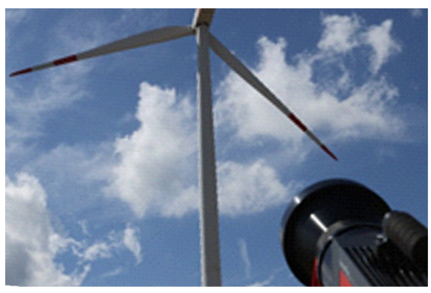
The used infrared camera is an IR8800-type from the manufacturer InfraTec GmbH (Gostritzer Str. 61-63, 01217 Dresden, Germany), which is sensitive to wavelengths between µm and has a noise-equivalent temperature difference (NETD) of mK. To achieve a sufficient image magnification, a telephoto lens is used for the field measurement. For the measuring distance of approximately an image field with , represented by px2, is the result. The evaluated rotor section was between and radial distance from the nacelle and the minimal chord length in the evaluated part is m. An in-process measurement is shown in Figure 1.

Figure 1.
The measurement setup with the IRT camera that aims at the wind turbine from a measuring distance of 190 m.
The field of view was fixed to the horizontal rotor position and the aforementioned radial rotor position, respectively. It covers the complete blade profile from the leading edge to the trailing edge. Triggering with an external visual camera has been previously reported and is possible, but here, the image acquisition is thermally triggered each time one of the rotor blades passes the defined region of interest due to an increased detected mean temperature within that region.
For comparable field measurements, the following requirements concerning the measurement and flow conditions are needed:
- The wind speed must be permanently between the switch-on and switch-off speed of the turbine. In addition, operation in the part-load range is desirable, since in part-load operation there is a linear dependence between the wind speed and the rotor speed and thus the optical detection of the rotor speed allows an approximation of the incident flow speed [31].
- The solar heating of the rotor blades is constant in time.
- For a fixed geometric alignment between the camera and the observed rotor blade section, no yawing or pitching may occur during the measurement period.
Therefore, the recorded image series are filtered with regard to these requirements, i.e., only time periods that meet the requirements are evaluated.
3.3. Signal Processing
The thermographic image acquisition is carried out using the IRBIS software (IRBIS professional 3.1.100) of the camera manufacturer InfraTec, while the Python software (3.9.18) is used for image processing. The correction of the image orientation is substantial for the application of the signal processing approaches in free field measurements. The correction of the image alignment includes the following image processing steps:
- Background removal and outlier removal.
- Detection of the rotor blade edges with Canny edge detection [32].
- Assignment of the edges (leading, trailing) via clustering and standard deviation within a cluster.
- Horizontal alignment of the leading edge by means of image rotation.
- Compensation of the interpolation effects on the image edges due to image rotation.
These preprocessing steps allow an evaluation of a thermogram both with (Section 2.2) and without (Section 2.1) previous knowledge for comparison reasons.
4. Results
The results are evaluated for images with different contrast-to-noise ratios (CNR). The CNR of an image is calculated as the average CNR value over all image columns, while the CNR of one column is calculated with the following equation:
where are the mean temperature values and are the standard deviations of the temperatures in the laminar and turbulent region of the rotor blade, respectively.
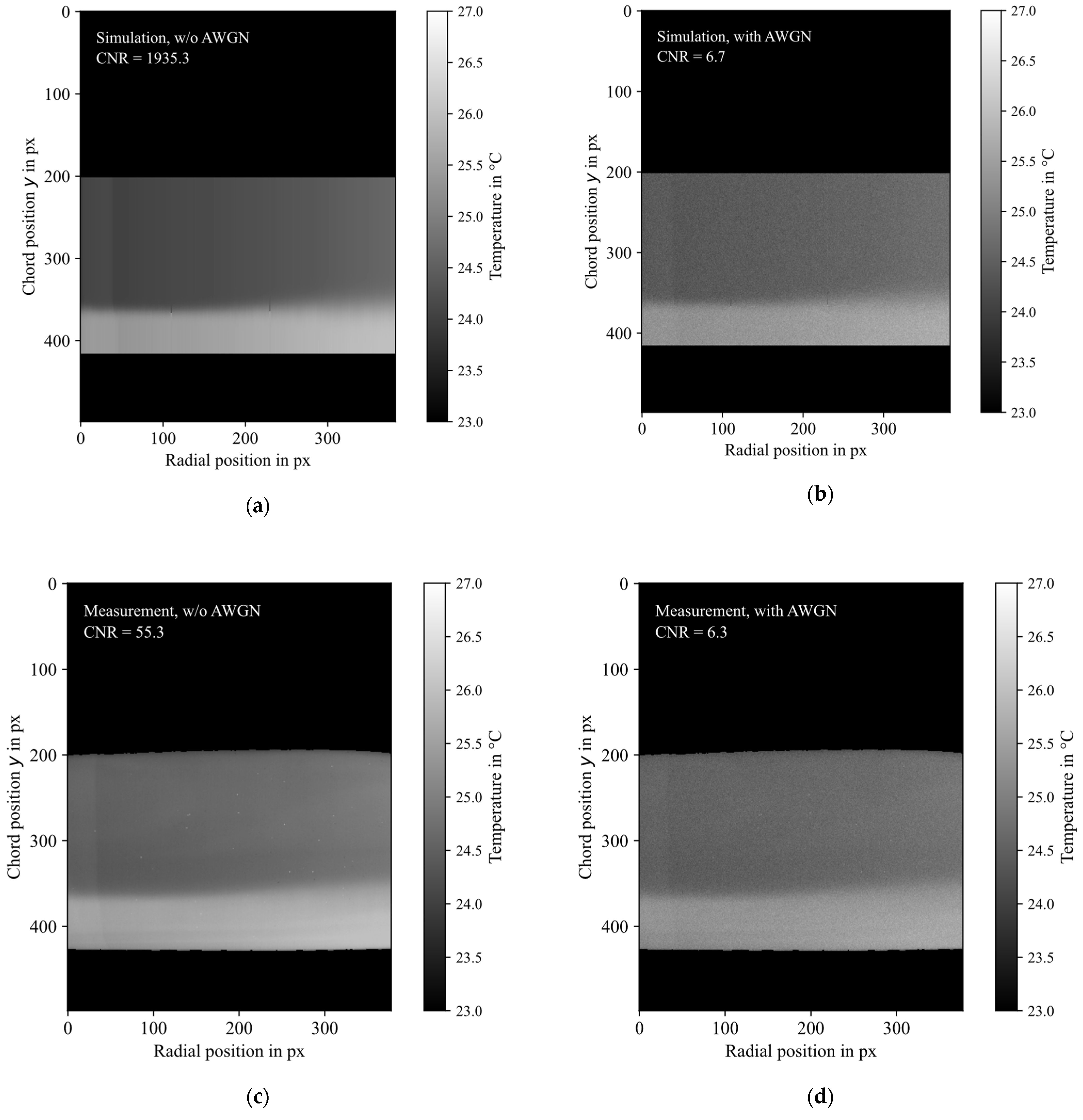
For verification and validation purposes, the Bayesian approach is tested on four kinds of data. First, a thermographic image is simulated, which means that the laminar–turbulent transition position is set manually, and the temperature values on the rotor blade exactly follow the error function introduced in Equation (2). This simulation process is carried out for every image column individually, which represents the chord axis. The simulated image is similar to the measurement (since it is designed on the basis of a measurement thermogram) but with an extraordinarily high CNR. As a result, the detected transition positions for the different image columns will always yield the given true value of the transition position for the simulated image. Second, a measured thermogram is used. Third and fourth, in order to evaluate the method on images of varying quality, which means thermograms with a different CNR, artificial Gaussian noise with the expectation value is added and the effect of different noise standard deviations is studied. As an example, Figure 2 shows, on the left, a simulated image (a) and a preprocessed thermogram with no added noise (c) and, thus, a high CNR value. At the right, the same images are shown with added noise, with a reduced similar CNR of 6.7 (b) and 6.3 (d), respectively. In Section 4.1, the simulation-based images are used to verify the Bayesian method for including previous knowledge and to compare its performance with the classical non-Bayesian estimation as a reference. Subsequently, in Section 4.2, the findings are validated for real, measured thermograms. Application scenarios to make use of the Bayesian method are presented in Section 4.3, which includes a discussion of suitable priors.
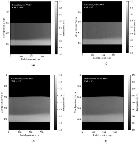
Figure 2.
Thermographic images: Simulated images with no (a) and with (b) added white Gaussian noise (AWGN). Measured thermograms with no (c) and with (d) added noise.
4.1. Verification of the Bayesian Approach
As a first indicator for the success of the Bayesian inference, the posterior distribution (Markov chain) of the transition position for the simulated image with noise and an informative prior with a mean value of px and a standard deviation of px is visually inspected and shown in Figure 3.
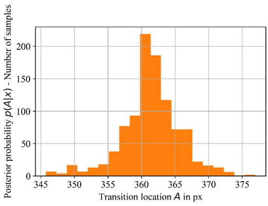
Figure 3.
Markov chain of the Bayesian analysis with at px and px.
The Bayesian posterior distribution of the proposed transition positions resembles a normal distribution with a mean value of px and a standard deviation of px. Indeed, a normal distribution with mean and standard deviation similar to the prior is expected, because, due to the high quality of the prior, the previous knowledge dominates the measurement data. Repetitive measurements show that the considered informative prior enables the determination of the transition position (px) with a standard deviation of px for a simulated image with a very low CNR of . Additionally, this standard deviation, which is achieved with previous knowledge, is lower than what is achieved with no previous knowledge (px).
The result is not surprising because the prior itself contains the true transition position with low uncertainty. However, the result verifies the Bayesian approach as a method for including previous knowledge into the thermogram evaluation for the determination of the laminar–turbulent transition position on rotor blades on wind turbines.
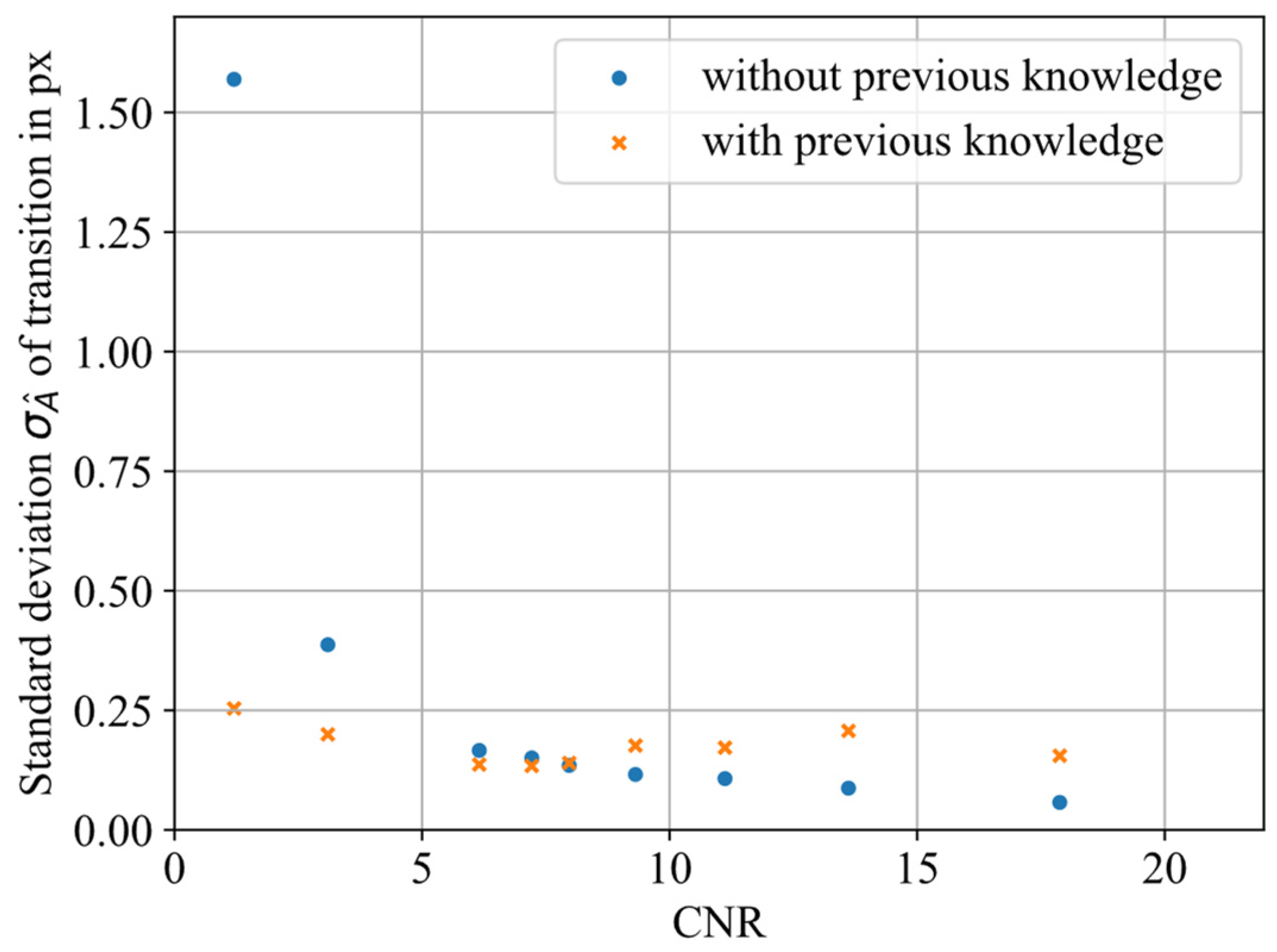
Next, the Bayesian method is evaluated with respect to the influence of the image quality, i.e., the CNR of the image. Repetitively, the transition position is determined with and without the use of previous knowledge for simulated images with different CNRs, which are created through a change in the standard deviation of the added Gaussian noise. The used prior is normally distributed with the mean at the true position and a standard deviation of px. As the added Gaussian noise has zero mean and is symmetric, it does not add any systematic error, and the obtained standard deviation of the flow transition position shown in Figure 4 (orange dots) can be interpreted as the standard measurement uncertainty.
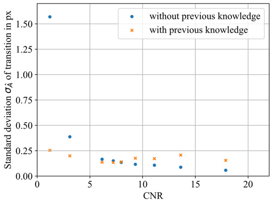
Figure 4.
Standard deviation of the determined laminar–turbulent transition position for different CNR values. The non-Bayesian (no previous knowledge) and the Bayesian (with previous knowledge) results are shown.
The quality of the reference signal evaluation without the use of previous knowledge (blue dots) depends on the CNR of the image and the standard deviation decreases with increasing CNR so that and . In the case of a low CNR < 7, previous knowledge (orange dots) clearly reduces the standard deviation . On the other hand, for high CNR values > 7, previous knowledge increases the standard deviation. This behavior is a common effect of the Bayesian inference for nonlinear models, which should vanish for high CNR values. To summarize, the prior knowledge dominates the measurement result for low CNR values, and the measurement data dominates for high CNR values. The use of previous knowledge is especially interesting, when it improves the measurement quality without dominating the result. Figure 4 shows that the measurement uncertainty is lowered for CNR values below 7, and the prior dominates when the CNR is below 3.
Generally, the prior’s quality is high when the mean value is close to the true value and when the prior has a small width (low uncertainty). In order to examine the prior influence on the posterior result, different priors are tested for a simulated image with CNR = 6.7, as shown in Figure 2b. All priors are normally distributed with the mean value at the true position so that only the standard deviation is varied. For this setup, the standard deviation of the prior stands for the quality of the prior. The determined measurement standard uncertainty of the transition position over the prior standard deviation is shown in Figure 5.
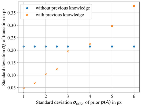
Figure 5.
Standard deviation of the determined laminar–turbulent transition position for different standard deviations of the prior for a simulated image with noise from Figure 2b.
The standard deviation of the transition position using the Bayesian method (orange dots) is only lower when the prior’s standard deviation is equal or lower than 3 px. For a prior of the determined transitions closely follow the priors mean value and, thus, the prior dominates the measurement. In contrast, for a prior of little quality (the standard deviation is higher with the use of previous knowledge. Generally, the Bayesian inference method should implicitly neglect the previous knowledge when it contains little information, and the results should then solely rely on the measurement data. Nevertheless, the necessity of a numerical calculation of the posterior function explains the increased standard deviation for a prior with high width. The results show that the prior’s quality is crucial for the success of the Bayesian method. In combination, the results in Figure 4 and Figure 5 provide a first approximation of the necessary balance between prior quality () and image quality (, where the use of previous knowledge lowers the measurement uncertainty for the localization of the laminar–turbulent transition on rotor blades of wind turbine.
4.2. Validation of the Bayesian Approach
In order to validate the findings from the study with the simulated images, the measured thermogram is now considered and superposed with noise (Figure 2d).
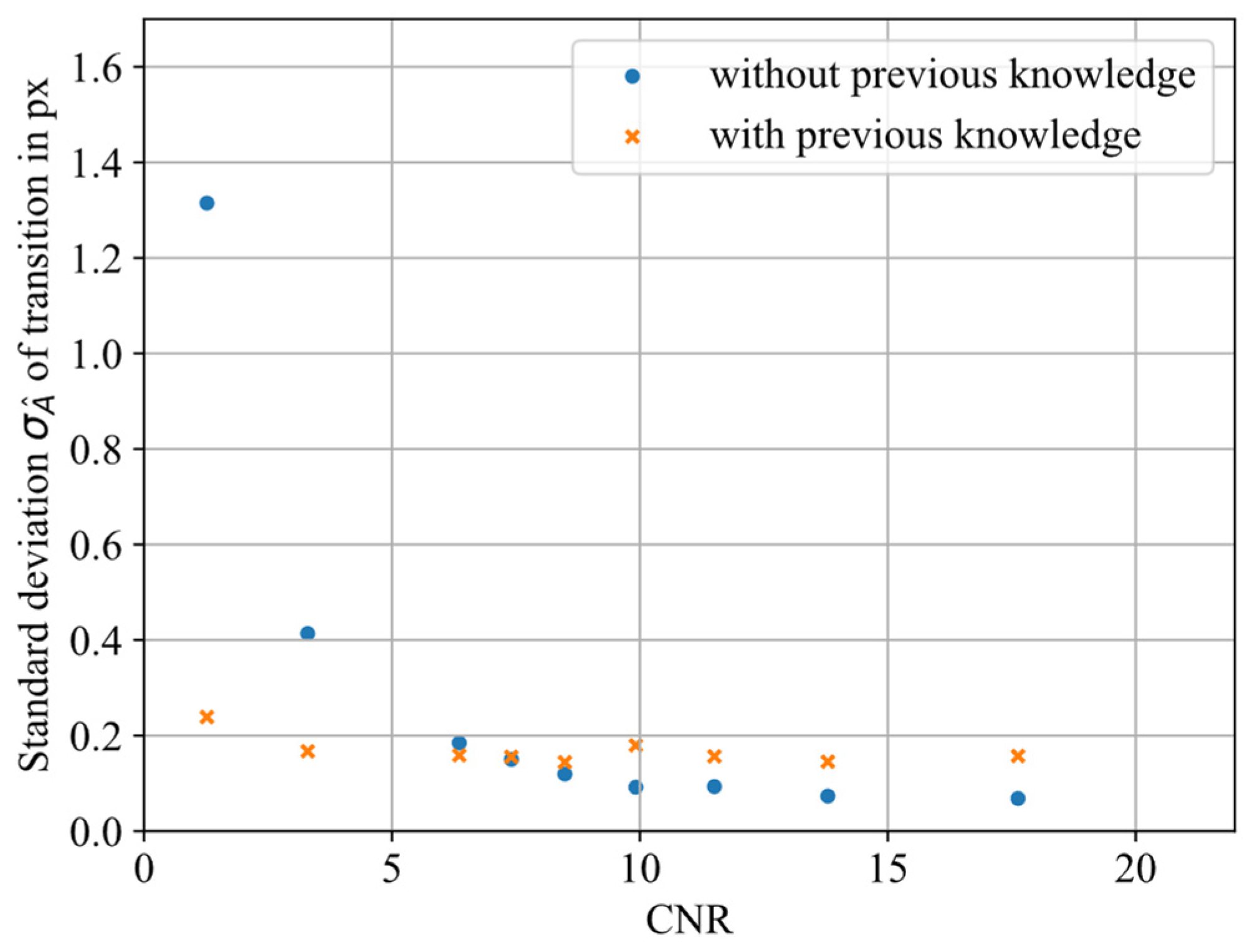
Figure 6 compares the standard deviation of determining the laminar–transition position on real measurement data with and without previous knowledge depending on the image quality. The standard deviation is lower with the use of previous knowledge for low CNRs, and the crossover point is at a CNR below 7, similar to Figure 4. The similarity validates the Bayesian inference as a method to lower the uncertainty of determining the position of the laminar–turbulent transition position on a noisy image.
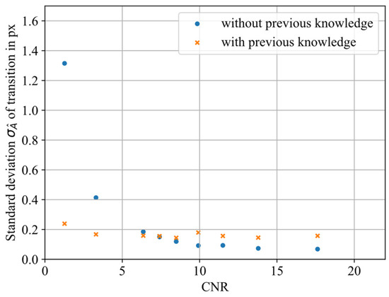
Figure 6.
Standard deviation for determining the transition position on thermographic images superposed with Gaussian noise for different CNR values.
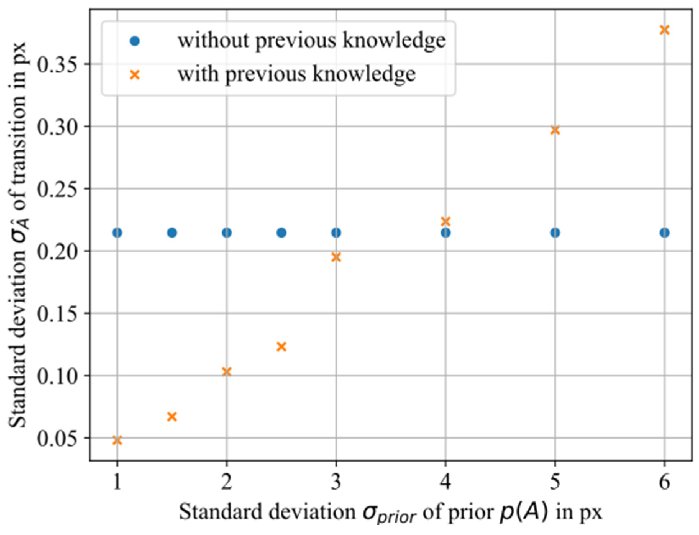
Figure 7 compares the standard deviation of determining the laminar–turbulent transition position on real measurement data with and without previous knowledge depending on standard deviation of the prior. In Figure 7 the standard deviation is lower for determining the laminar–turbulent transition position with the use of preknowledge when the standard deviation of the prior is . This validates the results from Figure 5 and, hence, validates the Bayesian inference as a method to lower the uncertainty when determining the position of the laminar–turbulent transition with an informative prior.
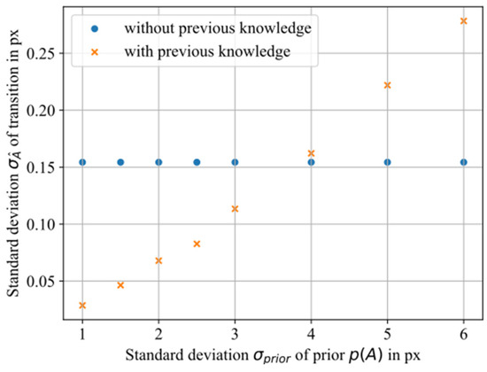
Figure 7.
Standard deviation for determining the transition position on thermographic images superposed with Gaussian noise for different standard deviation of the priors.
Summarizing and combining both findings from Figure 6 and Figure 7, the transition position uncertainty is lowered for images with a CNR below 7 and a normally distributed prior with a standard deviation smaller or equal to 3 px. If the prior has less quality or the image has a higher CNR, the Bayesian inference increases the uncertainty and should not be used.
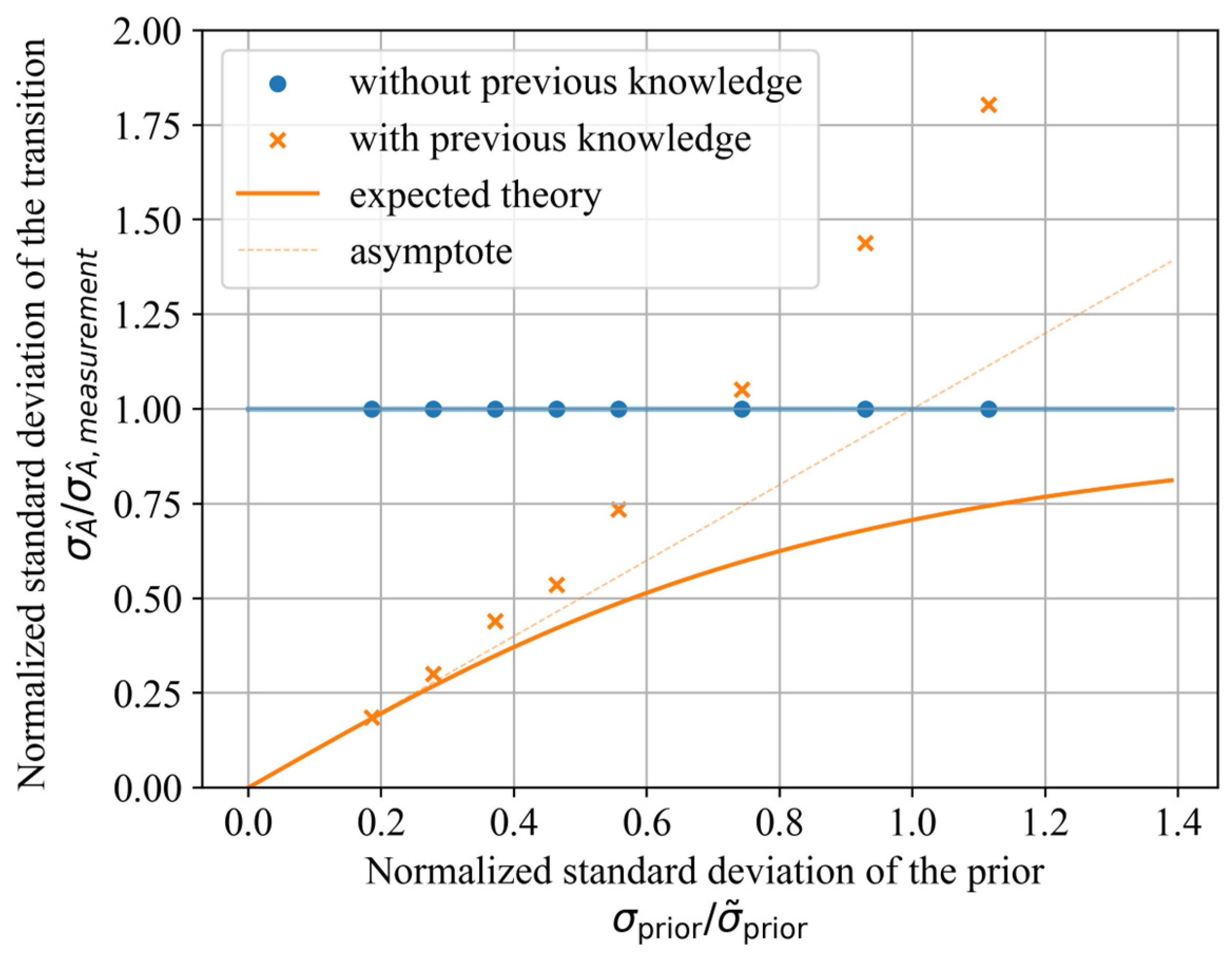
To compare the findings from Figure 7 with the expectations from estimation theory, the same data is shown again in Figure 8, but in a normalized manner. The ordinate is normalized by the standard deviation of the detected transition position without previous knowledge. The abscissa is normalized by the characteristic prior standard deviation , which is the point of intersection between the theoretical transition position standard deviation in case of a dominant previous knowledge (orange crosses: linear extrapolation through 0 and the first data point with minimal variance of the prior) and the transition position standard deviation with no previous knowledge (blue dots). For the studied example, = 5.4 px, which means that this prior is as informative as the measurement data.
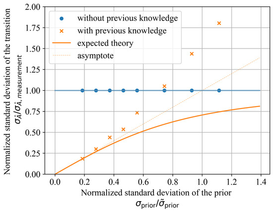
Figure 8.
Normalized standard deviation for determining the transition position on thermographic images superposed with Gaussian noise and comparison with the theoretical expectation from estimation theory [33], while considering different standard deviations of the prior (also normalized).
Hence, for a low standard deviation of the prior smaller than , the prior information should dominate the measurement result and the standard deviation of the detected transition position asymptotically should attain the standard deviation of the prior (orange dotted line). This theoretical expectation agrees with the experimental data.
For a high standard deviation of the prior larger than , where the information from the measurement data dominates, the standard deviation of the determined transition position should asymptotically reach , i.e., the same value as for the non-Bayesian evaluation. Specifically, the normalized standard deviation of the transition position is expected to obey the relation [33]
This is shown as a solid orange line. However, the experimental results of the implemented Bayesian evaluation do not follow the theoretical expectation for an increasing width of the prior. The assumed cause of this unexpected behavior is the insufficient calculation of the posterior, i.e., the numerical implementation of the Bayesian evaluation algorithm with limited resources in computational power and time, respectively. As a consequence, the nonlinearity and the complexity of the Bayesian evaluation requires an increasing calculation effort for an increasing width of the prior.
4.3. Application Scenarios and Suitable Priors
Previous knowledge can come from theory, simulations or previous experiments. In Section 4.1 and Section 4.2, it was shown that the quality of the previous knowledge decides whether it lowers the uncertainty for determining the laminar–turbulent transition position on rotor blades of wind turbines. The present section evaluates different scenarios on how previous knowledge may be gained and in what way it can or cannot improve the measurement of the laminar–turbulent transition position on rotor blades of wind turbines.
A proposed field of application for the Bayesian inference is to smoothen the spatial course of the flow transition position along the radial rotor blade position , which is the so-called transition line. The previous knowledge is obtained by combining all detected transition positions in a single image with a polynomial regression. In detail, the previous knowledge is defined to be normally distributed where the mean corresponds to a specific point on a polynomial curve along the radial axis and has a constant standard deviation . The polynomial is fitted onto the detected transition positions via least squares regression and the mean squared error of this regression is taken as the standard deviation of the prior.
By using the approximated course of the flow transition determined from the whole image as previous knowledge for the determination of the laminar–turbulent transition position, the resulting visualization of the transition line is expected to be less noisy.
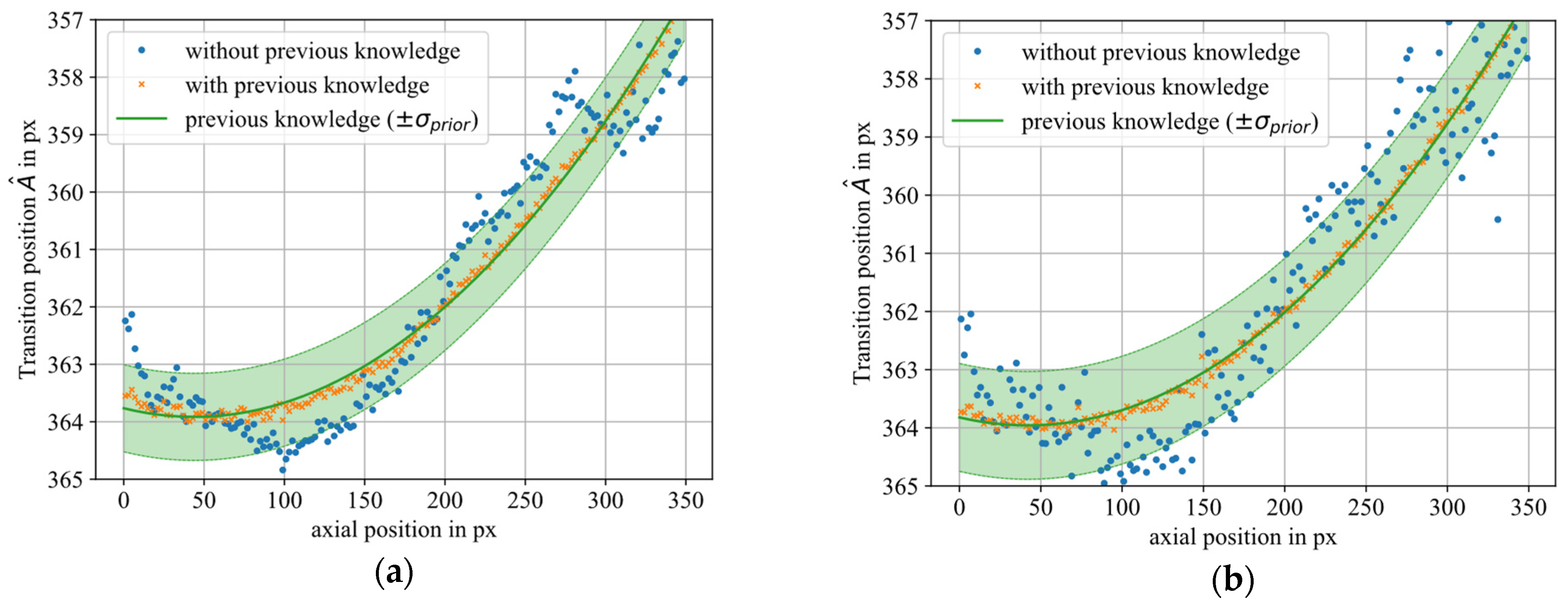
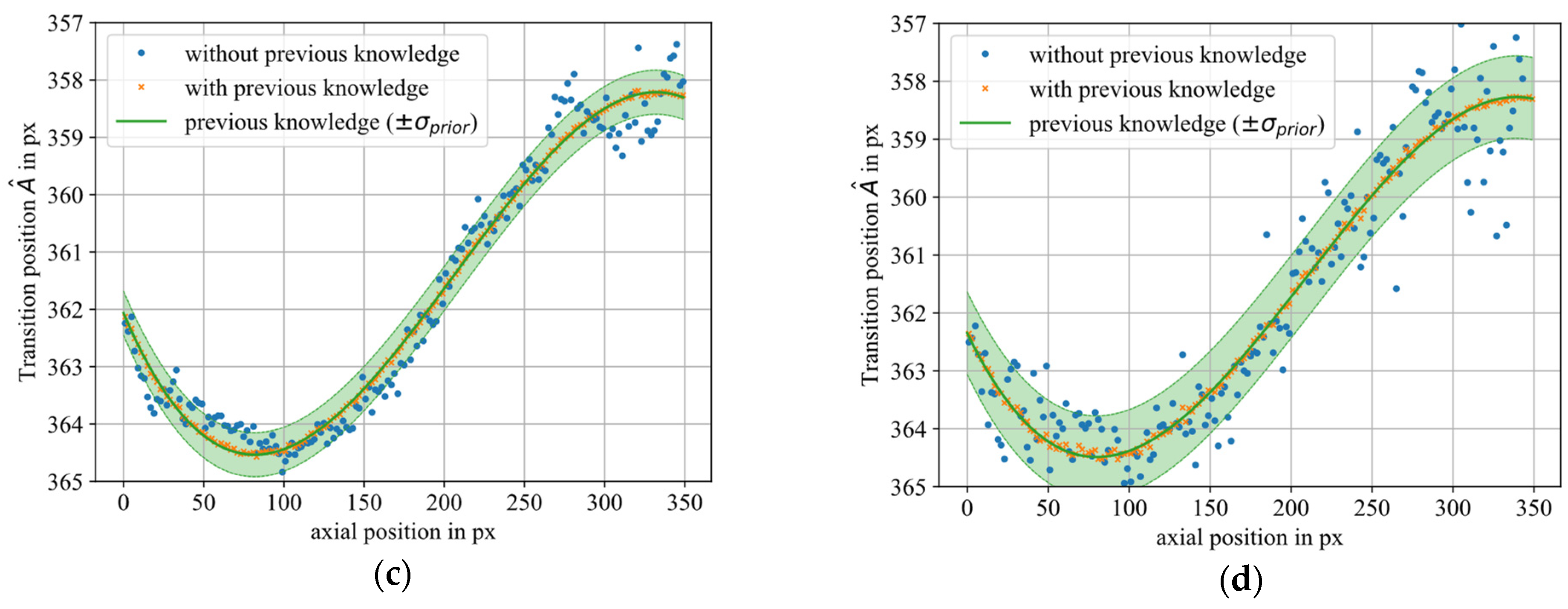
Each graph in Figure 9 shows the determined transition positions without previous knowledge in blue and with previous knowledge in orange. It further shows the mean of the prior as a solid line and the standard deviation of the prior as transparent interval in green. Figure 9 applies this method to a second-order polynomial (top row) and a third-order polynomial (bottom row). The left column of Figure 9 uses the measured thermogram (see Figure 2c) and the right column uses a thermogram with noise (similar to Figure 2d).

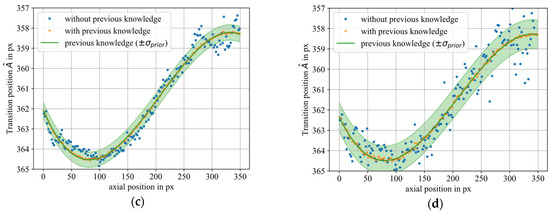
Figure 9.
The course of laminar–turbulent transition line over the axial rotor blade position, while the transition positions are determined with (orange) and without (blue) previous knowledge, respectively. The mean and the interval of the prior is additionally shown in green. The previous knowledge of the transition line is obtained with a polynomial regression with the order of 2 (a) and 3 (c). The case of a lower signal-to-noise ratio is studied in (b,d), where noise has been added to the original measurement data.
Through individually calculating the laminar–turbulent transition position for each column without sacrificing the spatial resolution, the application of the Bayesian method results in a smoother visualization of the transition line. Additionally, the Markov chain is an implicit uncertainty evaluation of the Bayesian result. However, in the example, the measured data has little influence on the result because the posterior result sticks very close to the chosen prior. The determined transition positions with prior information that follows a second order polynomial leave the course of the non-Bayesian measurement, which presumable introduces a systematic error (although the true value is not known here). The explanation is that the information within the prior is stronger than the measurement causing a prior-dominated result. Thus, the Bayesian inference can be used to visualize the transition line with less noise, but the result is dominated by the information within the prior so that it resembles a polynomial regression.
Whereas the last result generated knowledge through averaging spatial position information from a single image, another idea is to use temporally related results from former experiments to form previous knowledge on the temporal course of the flow transition position. Exemplary, the transition position has been determined 150 times within an hour to determine mean value and standard deviation of the normally distributed prior for the subsequent position measurements. This means a constant transition position over time is assumed here as an example, and the prior information comes solely from the past. The prior is applied for the evaluation of the measurements of the following hour. It is important that the previous knowledge and the measurement are taken under the same conditions. In the measurement it was made sure that between the generation of previous knowledge and the measurement the wind turbine did not yaw or pitch and the wind speed constantly was between 3 m/s and 8 m/s. Figure 10 shows the relative measured transition position (0—leading edge; 1—trailing edge) for 150 randomly chosen moments within 60 min with and without the use of the previous knowledge.
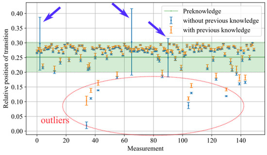
Figure 10.
Laminar–turbulent transition position with standard deviation for 50 measurements with and without the use of previous knowledge.
For 90% of the measurements, the standard deviation (shown by the error bars) is smaller without the use of previous knowledge and the determined transition positions seem plausible. Thus, the use of previous knowledge does not lower the uncertainty of these measurements. However, for measurements with an extraordinary random error (marked with blue arrows) the use of previous knowledge gained from former experiments strongly lowers the uncertainty of the measurement. In addition, measurements occur (within the red dotted ellipsis), where the determined transition position is significantly apart from the mean position. As the true value is not known, it cannot be concluded if this is due to an actual change in the transition or due to an error in the measurement. Assuming the measurements in the red dotted circle to be falsely detected transition positions, then the use of previous knowledge also lowers the systematic error for the measurement. As a result, previous knowledge gained through former experiments can be incorporated with the Bayesian inference to reduce the measurement uncertainty of erroneous detections of the flow transition position. Thereby, the Bayesian result incorporates an implicit uncertainty evaluation in the Markov chain.
As a summary, Table 1 compares the advantageous and disadvantageous features of determining the laminar–turbulent transition on rotor blades of wind turbines with Bayesian and classical, non-Bayesian estimation methods. It is important to note that the possibilities of Bayesian estimation may be expanded by finding alternative sources of previous knowledge in the future.

Table 1.
This table qualitatively compares the Bayesian estimation for the use of previous knowledge with two classical estimation approaches, which are the least squares estimation from Dollinger et al. and its combination with a principal component analysis method from Gleichauf et al. [19]. It compares the advantages and limits of all methods.
5. Conclusions
The primary contribution of this work is to provide a framework for the use of previous knowledge for determining the laminar–turbulent transition on rotor blades of wind turbines by means of thermographic flow visualization.
The Bayesian inference is verified and validated as a method to use previous knowledge to lower the position uncertainty of the laminar–turbulent transition on rotor blades of wind turbines. As a result, using previous knowledge reduces the uncertainty for determining the laminar–turbulent transition position on rotor blades when the measured thermogram provides an image with a low CNR. However, the width of the distribution of the previous knowledge is crucial. For the studied measurement data, a normally distributed prior needs to have a standard deviation px in order to improve the measurement on a thermogram with a CNR of 7. As a potential application, the Bayesian-based image processing enables a smoothening of the course of the transition position data along a rotor blade and over time, respectively, where the determination without previous knowledge produces implausible results. The previous knowledge can be obtained from the spatially or temporally neighboring data, but must be taken under the same measurement conditions as the measurement itself. Furthermore, the Markov chain implicitly provides a probability distribution for the measurand and, thus, a measure for the uncertainty of the Bayesian result.
Future investigations should focus on how previous knowledge can be extracted from flow simulations or experiments that fulfill the above-mentioned criteria. Comparing the standard deviation of a newly generated prior and the CNR of the measurement to the results from this publication allows for an evaluation whether the quality of the prior lowers the uncertainty of determining the laminar–turbulent transition position. In addition, it is of great interest to research whether the Bayesian inference can be used to observe a moving transition line resulting from unsteady inflow conditions or to detect further fluid-dynamic phenomena such as stall.
Author Contributions
Conceptualization: J.D., A.v.F. and A.F.; methodology: J.D. and A.F.; software: J.D.; validation: J.D., C.D. and N.B.; formal analysis: J.D. and A.F.; investigation: J.D. and C.D.; resources: J.D. and N.B.; data curation: J.D. and C.D.; writing—original draft preparation: J.D., A.v.F. and A.F.; writing—review and editing: J.D., C.D., N.B., A.v.F. and A.F.; visualization: J.D. and A.v.F.; supervision: A.v.F. and A.F.; project administration: J.D., A.v.F. and A.F.; funding acquisition: A.v.F. and A.F. All authors have read and agreed to the published version of the manuscript.
Funding
This research was funded by the Federal Ministry of Education and Research (BMBF), grant number 03SF0687A.
Institutional Review Board Statement
Not applicable.
Informed Consent Statement
Not applicable.
Data Availability Statement
The data presented in this study are available on request from the corresponding authors. The data are not publicly available due to privacy.
Conflicts of Interest
Author Nicholas Balaresque was employed by the company WindGuard Engineering GmbH. The remaining authors declare that the research was conducted in the absence of any commercial or financial relationships that could be construed as a potential conflict of interest.
References
- Schlichting, H.; Gersten, K. Grenzschicht-Theorie: Mit…22 Tabellen; 10., Überarb. Aufl; Springer: Berlin/Heidelberg, Germany, 2006. [Google Scholar]
- Schaffarczyk, A.P.; Schwab, D.; Breuer, M. Experimental detection of laminar-turbulent transition on a rotating wind turbine blade in the free atmosphere. Wind Energy 2016, 20, 211–220. [Google Scholar] [CrossRef]
- Meyers, J.F. Development of Doppler global velocimetry as a flow diagnostics tool. Meas. Sci. Technol. 1995, 6, 769–783. [Google Scholar] [CrossRef]
- Fischer, A. Model-based review of Doppler global velocimetry techniques with laser frequency modulation. Opt. Lasers Eng. 2017, 93, 19–35. [Google Scholar] [CrossRef]
- Kompenhans, J.; Reichmuth, J. 2-D flow field measurements in wind tunnels by means of particle image velocimetry. In International Congress on Applications of Lasers & Electro-Optics; Laser Institute of America: San Diego, CA, USA, 1987; pp. 119–126. [Google Scholar] [CrossRef]
- Gartenberg, E.; Roberts, A.S. Airfoil Transition and Separation Studies Using an Infrared Imaging System. J. Aircr. 1991, 28, 225–230. Available online: https://ntrs.nasa.gov/citations/19910055592 (accessed on 26 April 2023). [CrossRef]
- Montelpare, S.; Ricci, R. A thermographic method to evaluate the local boundary layer separation phenomena on aerodynamic bodies operating at low Reynolds number. Int. J. Therm. Sci. 2004, 43, 315–329. [Google Scholar] [CrossRef]
- Gartenberg, E.; Roberts, A.S., Jr.; McRee, G.J. Infrared imaging and tufts studies of boundary layer flow regimes on a NACA 0012 airfoil. In ICIASF 1989—13th International Congress on Instrumentation in Aerospace Simulation Facilities; IEEE: Piscataway, NJ, USA, 1989; pp. 168–178. [Google Scholar]
- Gazzini, S.L.; Schädler, R.; Kalfas, A.I.; Abhari, R.S. Infrared thermography with non-uniform heat flux boundary conditions on the rotor endwall of an axial turbine. Meas. Sci. Technol. 2016, 28, 025901. [Google Scholar] [CrossRef]
- Von Hoesslin, S.; Stadlbauer, M.; Gruendmayer, J.; Kähler, C.J. Temperature decline thermography for laminar–turbulent transition detection in aerodynamics. Exp. Fluids 2017, 58, 129. [Google Scholar] [CrossRef]
- Horstmann, K.H.; Quast, A.; Redeker, G. Flight and wind-tunnel investigations on boundary-layer transition. J. Aircr. 1990, 27, 146–150. [Google Scholar] [CrossRef]
- Dollinger, C.; Sorg, M.; Balaresque, N.; Fischer, A. Measurement uncertainty of IR thermographic flow visualization measurements for transition detection on wind turbines in operation. Exp. Therm. Fluid Sci. 2018, 97, 279–289. [Google Scholar] [CrossRef]
- Reichstein, T.; Schaffarczyk, A.P.; Dollinger, C.; Balaresque, N.; Schülein, E.; Jauch, C.; Fischer, A. Investigation of Laminar–Turbulent Transition on a Rotating Wind-Turbine Blade of Multimegawatt Class with Thermography and Microphone Array. Energies 2019, 12, 2102. [Google Scholar] [CrossRef]
- Oehme, F.; Gleichauf, D.; Suhr, J.; Balaresque, N.; Sorg, M.; Fischer, A. Thermographic detection of turbulent flow separation on rotor blades of wind turbines in operation. J. Wind. Eng. Ind. Aerodyn. 2022, 226, 105025. [Google Scholar] [CrossRef]
- Oehme, F.; Gleichauf, D.; Balaresque, N.; Sorg, M.; Fischer, A. Thermographic detection and localisation of unsteady flow separation on rotor blades of wind turbines. Front. Energy Res. 2022, 10, 1043065. [Google Scholar] [CrossRef]
- Raffel, M.; Merz, C.B. Differential Infrared Thermography for Unsteady Boundary-Layer Transition Measurements. AIAA J. 2014, 52, 2090–2093. [Google Scholar] [CrossRef]
- Gleichauf, D.; Oehme, F.; Parrey, A.-M.; Sorg, M.; Balaresque, N.; Fischer, A. On-site contactless visualization of the laminar-turbulent flow transition dynamics on wind turbines. tm Tech. Mess. 2023, 90, 9. [Google Scholar] [CrossRef]
- Gleichauf, D.; Dollinger, C.; Balaresque, N.; Gardner, A.D.; Sorg, M.; Fischer, A. Thermographic flow visualization by means of non-negative matrix factorization. Int. J. Heat Fluid Flow 2020, 82, 108528. [Google Scholar] [CrossRef]
- Gleichauf, D.; Oehme, F.; Sorg, M.; Fischer, A. Laminar-Turbulent Transition Localization in Thermographic Flow Visualization by Means of Principal Component Analysis. Appl. Sci. 2021, 11, 5471. [Google Scholar] [CrossRef]
- Mohammady, M.H.; Miyadera, T. Quantum measurements constrained by the third law of thermodynamics. Phys. Rev. A 2023, 107, 022406. [Google Scholar] [CrossRef]
- Bayes, T.; Price, R. LII. An essay towards solving a problem in the doctrine of chances. By the late Rev. Mr. Bayes, F. R. S. communicated by Mr. Price, in a letter to John Canton, A. M. F. R. S. Phil. Trans. R. Soc. 1763, 53, 370–418. [Google Scholar] [CrossRef]
- Gelfand, A.E.; Smith, A.F.M. Sampling-Based Approaches to Calculating Marginal Densities. J. Am. Stat. Assoc. 1990, 85, 398–409. [Google Scholar] [CrossRef]
- Meija, J.; Bodnar, O.; Possolo, A. Ode to Bayesian methods in metrology. Metrologia 2023, 60, 052001. [Google Scholar] [CrossRef]
- Kruschke, J.K. Bayesian Assessment of Null Values Via Parameter Estimation and Model Comparison. Perspect. Psychol. Sci. 2011, 6, 299–312. [Google Scholar] [CrossRef] [PubMed]
- Attivissimo, F.; Giaquinto, N.; Savino, M. Some Thoughts About the Frequentist and the Bayesian Approach to Uncertainty. In Proceedings of the XVIII IMEKO TC-4 Symposium, Natal, Brazil, 27–30 September 2011. [Google Scholar]
- Lira, I.; Grientschnig, D. Bayesian assessment of uncertainty in metrology: A tutorial. Metrologia 2010, 47, R1–R14. [Google Scholar] [CrossRef]
- Cowen, S.E.; Wilson, P.; Pennecchi, F.; Kok, G.; van der Veen, A.; Pendrill, L. A Guide to Bayesian Inference for Regression Problems; PTB: Braunschweig, Germany, 2015. [Google Scholar]
- Gilks, W.; Richardson, S.; Spiegelhalter, D. Introducing Markov Chain Monte Carlo; CRC Press: Boca Raton, FL, USA, 1996. [Google Scholar]
- University of Maryland. Change of Random Variables. Available online: https://www.math.umd.edu/~millson/teaching/STAT400fall18/handouts/changeofvariable.pdf (accessed on 28 April 2023).
- Weir, M.D.; Hass, J.; Thomas, G.B. Thomas’ Calculus: Early Transcendentals, 13th ed.; Pearson: Boston, MA, USA, 2014. [Google Scholar]
- Halyani, M.Y.; Firdaus, H.M.S.; Azizi, M.S.; Tajul, A.; Farhana, R.F. Modeling and Simulation of Wind Turbine for Partial Load Operation. ARPN J. Eng. Appl. Sci. 2016, 11, 4934–4941. [Google Scholar]
- Canny, J. A Computational Approach to Edge Detection. IEEE Trans. Pattern Anal. Mach. Intell. 1986, 8, 679–698. [Google Scholar] [CrossRef]
- Kay, S.M.; Kay, S.M. Fundamentals of Statistical Signal Processing. 1: Estimation Theory; 20. Pr; Prentice Hall PTR: Upper Saddle River, NJ, USA, 2013. [Google Scholar]


Disclaimer/Publisher’s Note: The statements, opinions and data contained in all publications are solely those of the individual author(s) and contributor(s) and not of MDPI and/or the editor(s). MDPI and/or the editor(s) disclaim responsibility for any injury to people or property resulting from any ideas, methods, instructions or products referred to in the content. |
© 2024 by the authors. Licensee MDPI, Basel, Switzerland. This article is an open access article distributed under the terms and conditions of the Creative Commons Attribution (CC BY) license (https://creativecommons.org/licenses/by/4.0/).