A Theoretical Method for Calculating the Internal Contact Pressure of Parallel Wire Cable during Fretting Wear

Abstract

Fretting wear of the stay cable is an important factor affecting the service life of the cable. To accurately calculate the extent of fretting wear, it is necessary to calculate the internal contact pressure in the cable. Although there are many theories and experiments on the contact behavior between wires, there are still no theoretical formulations for calculating the distribution of contact pressure in stay cables. In this paper, by studying the transfer effect of contact pressure in the cable, the PIC (parallel wire cable internal point contact pressure) model for calculating the contact pressure in the parallel wire cable is proposed, considering the effects of wire twisting, sheath compression, and cable bending on the contact pressure. A finite element model corresponding to the contact mode between steel wires is established, and the effectiveness of the PIC model is verified through numerical simulation analysis and a comparison of the existing contact models. The results indicate that contact pressure caused by wire twisting (CWT) is superimposed layer by layer inwards, with the contact pressure increasing closer to the inner layers, and its magnitude is mainly related to the axial tension and twist angle. Simultaneously, on the same layer, contact points along the diagonal experience the greatest contact pressure. Contact pressure caused by sheath compression (CSC) is assumed to conform to the Boussinesq distribution, with the outer layers exhibiting greater contact pressure compared to the inner layers. Contact pressure caused by cable bending (CCB) conforms to the two-dimensional closely arranged contact force transmission model, has a clear layering phenomenon, and the contact pressure within the same layer does not change significantly. The magnitude of the contact pressure is exponentially related to the curvature of the cable and proportional to the tension of the cable, which explains the reason why the slip occurs later for the cables with high tensile forces. Among these three types of contact pressure, CWT is the greatest, followed by CCB, while CSC is the smallest. The theoretical analysis results show that factors such as wire radius, tension, torsion angle, and wire position have an impact on contact pressure. Contact pressure is transmitted along force chains within the cable, following the superposition law between layers. It is uncertain whether slip occurs in the neutral axis or in the outermost layer because of the different distributions of tangential force and interlayer frictional resistance between the layers of wires. Fretting wear simulations of two wires demonstrate that contact pressure has a significant influence on wear patterns, and the “averaging” of contact pressure is a major reason for achieving uniform interface wear. While the contact width increases proportionally with the contact pressure, excessive contact pressure can complicate the problem by changing the contact mode from gross slip to partial slip. This study provides a theoretical method for calculating contact pressures at any contact point within the cables in engineering practice.

1. Introduction

As the primary load-bearing components of cable-stayed bridges, the durability of the stay cables directly influences the service life of the entire structure [1]. During the operation stage of a cable-stayed bridge, external loads induce vibrations in the stay cables, leading to relative movement among the internal wires and consequently giving rise to fretting wear [2]. This phenomenon results in a reduction in the strength and durability of the cables, markedly impacting the overall lifespan of the cable-stayed bridge. Assessing the degree of wire damage by studying the fretting wear behavior within the stay cable, and timely replacing stay cables with insufficient strength ensure the safety of the cable-stayed bridge during its operation stage.

Fretting wear is influenced by various factors such as contact pressure, displacement amplitude, and motion frequency. Among these, contact pressure determines the size of the initial contact area, stress field, and tangential stiffness, etc. [3], making it a crucial parameter in studying the laws of fretting wear. Through experiments involving the wear of two wires, including both vertical point contact [4,5,6,7] and parallel line contact [8,9], it has been demonstrated that the contact pressure between wires not only affects the developmental patterns of friction coefficients and wear coefficients but also, with an increase in contact pressure, induces alterations in the sliding state of the wire contact interface, consequently further diminishing the service life of the cable [10]. In the actual operation of cable-stayed bridges, the dynamic monitoring of contact pressure proves challenging, often leading to an underestimation of the impact of fretting wear, particularly on cable damage, including corrosion [11,12] and fatigue [13,14]. Preliminary findings from relevant experimental studies have elucidated the influence of contact pressure between wires on fretting wear.

The theoretical exploration of contact pressure between wires originated from the study of failure modes in wire ropes [15,16,17,18,19,20,21]. Huang et al. [22], by examining the tensile condition and separation trend of wires during stretching and twisting, analyzed the wire contact patterns and derived the contact pressure between the core wire and helical wires. Gnanavel et al. [23], based on Love’s slender rod equilibrium principles, established a radial contact model for stranded cables, elucidating the impact of contact pressure on axial strain and torsional slip of the wires. When considering multi-layer scenarios, LeClair et al. [24], employing Hertz contact theory and contact mechanics, derived a theoretical model for interlayer contact forces. These theoretical models serve as crucial reference tools for computing the contact pressure in wire ropes.

Unlike wire ropes, the application of a parallel wire cable system is more prevalent in cable-stayed bridges. Despite numerous theoretical models and experimental measurements [25,26,27,28,29,30,31,32,33,34], the existing methods for calculating the internal contact pressure within parallel wire cable still exhibit certain limitations. This is primarily because most of the previous studies have focused solely on the local pressure distribution at the contact interface of two wires [25,26,27,28,29,30,31], neglecting an analysis of the transmission of contact pressure throughout the entire cable. They overlooked the cumulative effects of contact pressure from the outer layers to the inner layers. In practical parallel wire cables, there are often dozens or even hundreds of wires, with studies thus necessitating consideration of the mutual interactions resulting from their contacts. Furthermore, many studies have overlooked the radial compression effect caused by the cooling of the sheath during the production of the stay cable, as well as the wire extrusion effect due to cable vibration and bending during usage [32,33,34]. This results in underestimated contact pressure values, leading to an underestimation of damage caused by fretting wear.

In response to these circumstances, this study has devised a model denoted as PIC (parallel wire cable internal point contact pressure) to compute the contact pressure between internal wires in the cable. Diverging from conventional methods that derive contact force from strain, this model calculates the inter-wire contact pressure induced by wire torsion by analyzing the transmission pathways of twisting forces within the cables. It employs Boussinesq distribution to calculate the radial contact pressure resulting from sheath compression and, based on a two-dimensional closely arranged contact force transmission model, computes the interlayer contact pressure caused by cable vibration and bending. Consequently, the specific formula for calculating contact pressure is derived. Through this methodology, contact pressure at different contact points within parallel wire cable can be determined. Compared to previous theories, this approach is more comprehensive, incorporating a superimposed analysis of contact force transmission, yielding results closer to real-world conditions. Building upon theoretical calculations, numerical simulation analyses are conducted on various contact models, revealing the distribution patterns of contact pressure on the cross-section of the cable strands. Finally, finite element models for fretting wear of two wires are established, analyzing the influence of contact pressure on wear depth and wear radius. This theoretical model holds promise in guiding the calculation of internal contact pressure distribution in engineering practice involving cable strands.

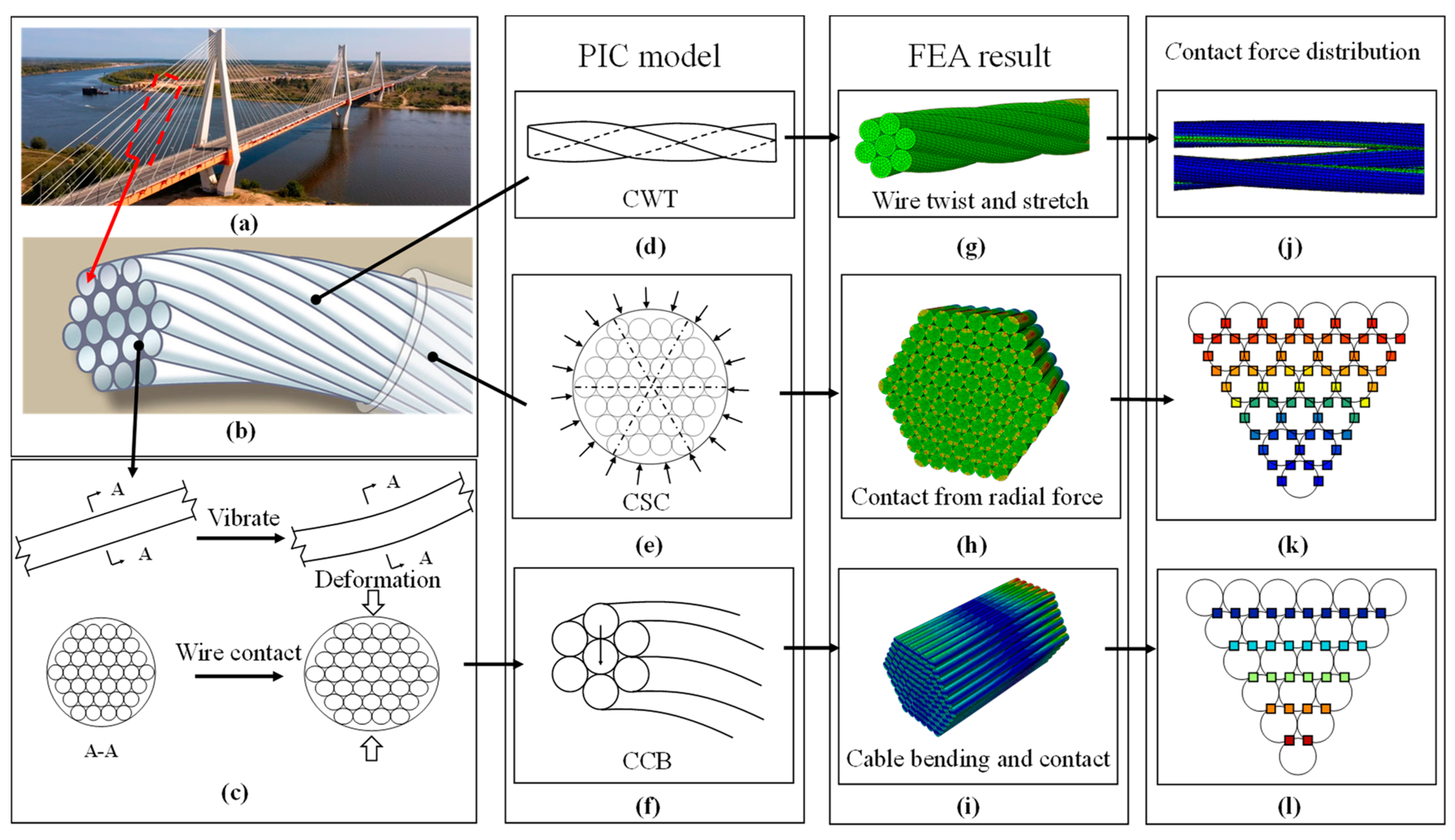
2. Theoretical Derivation of PIC Model

Fretting wear can profoundly impact the service life of cable-stayed structures. To quantitatively assess the extent of fretting wear, it is imperative to calculate the contact pressure at each contact point within the cable-stayed system. The general idea of this paper is illustrated in Figure 1. To comprehensively consider the diverse factors influencing the contact pressure between wires, this paper classifies contact pressure into three types based on their sources. Corresponding methods for calculating contact pressure under each circumstance were derived. Subsequently, finite element simulations were conducted in later sections, wherein the distribution patterns of contact pressure across the entire cross-section of the cable were discussed.

Specifically, during the manufacturing process, parallel wires in the cable-stayed system undergo concentric leftward twisting after bundling. Subsequently, a high-density polyethylene sheath is thermally extruded onto the outer surface of the wire bundle. In this process, internal parallel wires experience inward extrusion pressure, giving rise to contact forces. During the normal operation stage of the cable-stayed structure, the cables undergo bending due to vibration, leading to contact extrusion of internal parallel wires, and consequently generating contact pressure. From these three aspects, three sources of contact pressure between the wires can be obtained:

• Contact pressure caused by wire twisting (CWT): contact pressure generated by the twisting of parallel wires during the manufacturing process;
• Contact pressure caused by sheath compression (CSC): constriction due to external radial forces, such as sheath and clamp;
• Contact pressure caused by cable bending (CCB): contact of wires in different layers caused by the bending during the operation stage.

2.1. Basic Rules in Theoretical Derivation of PIC Model

This paper takes parallel wires $91\varphi 7$ as an example, commonly utilized in engineering practice. As Figure 2 shows, the positions of the wires on the cable cross-section are denoted by $\left(i,j\right)$, and the six contact points with the surrounding wires are indicated by $〈k〉$.

In addition, the following assumptions are followed in the theoretical derivation:

• Tight contact is maintained between the wires.
• Only the twisting effect of the wires is considered, disregarding torsion resulting from tension.
• The radial force generated by sheath compression is uniform.
• Wire deformation adheres to the assumption of a flat cross-section, neglecting shear deformation arising from wire bending.

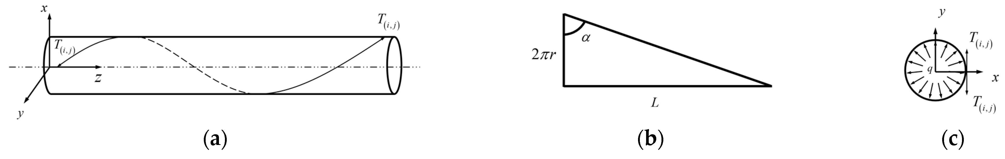
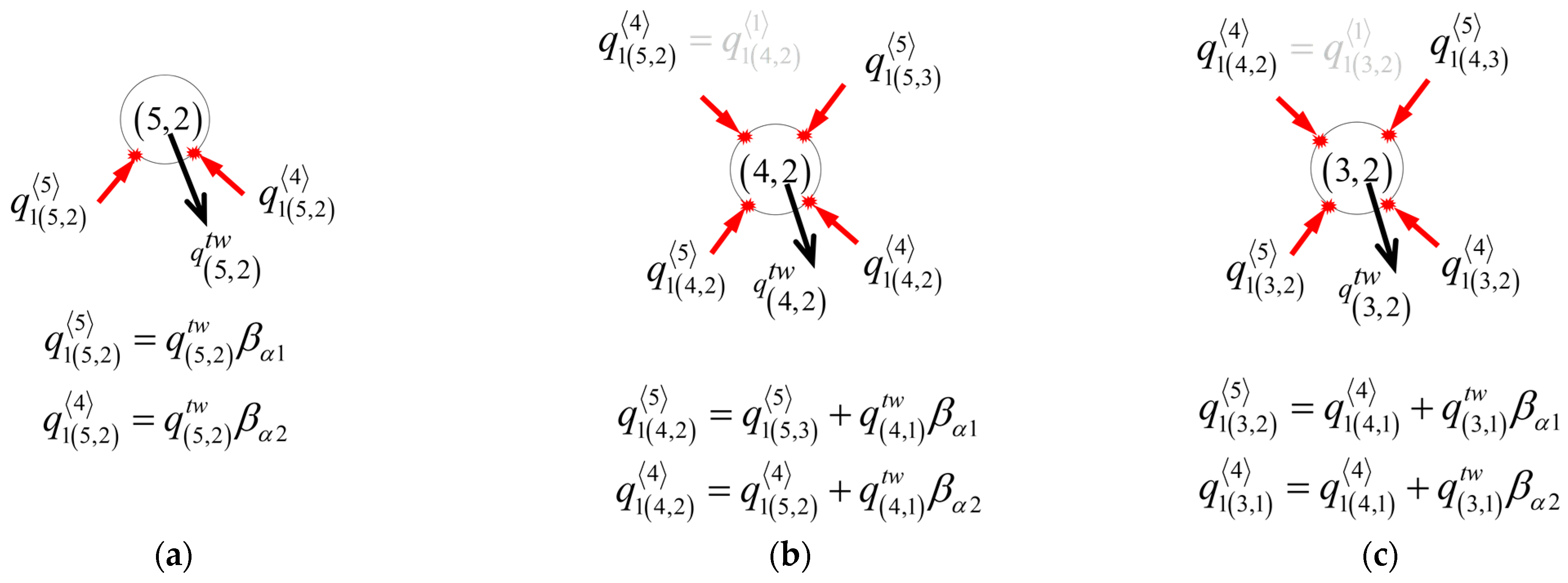
2.2. Contact Pressure Caused by Wire Twisting

The primary source of contact pressure between wires is the extrusion force caused by wire twisting. When calculating the contact pressure caused by the twisting of wires, the primary consideration lies in the axial tension exerted on the outer wire, giving rise to the radial contact pressure on the inner wire. As Figure 3 shows, in the formation of the cable, the wires undergo slight twisting, each winding in a helical form around the inner layer of wires. At this point, the tangential tension in $\left(i,j\right)$ wire is denoted as $T_{\left(i,j\right)}$, the twisting angle is represented by ${\alpha }_{\left(i,j\right)}$, and the twisting force per unit length is given by $q_{\left(i,j\right)}^{tw}$ [29,34]:

$$q_{\left(i,j\right)}^{tw}=\frac{T_{\left(i,j\right)}}{r\left(1+{\tan }^2{\alpha }_{\left(i,j\right)}\right)}=\frac{T_{\left(i,j\right)}}{r}\cdot {\cos }^2{\alpha }_{\left(i,j\right)}$$

(1)

The twisting force $q_{\left(i,j\right)}^{tw}$ is directed towards the center of the cable cross-section. Each wire not only bears the extrusion contact pressure generated by the twisting of the upper layer but also transmits this contact pressure, along with its own twisting force, to the lower layer of wires. Assuming complete transmission of this contact force, the contact pressure at different contact points can be obtained by superimposing the twisting forces of different layers of wires.

When calculating the contact pressure at a specific point, it is necessary to consider the specific location of that point on the cable cross-section. Contact points can be classified into two types based on their positions: diagonal and non-diagonal.

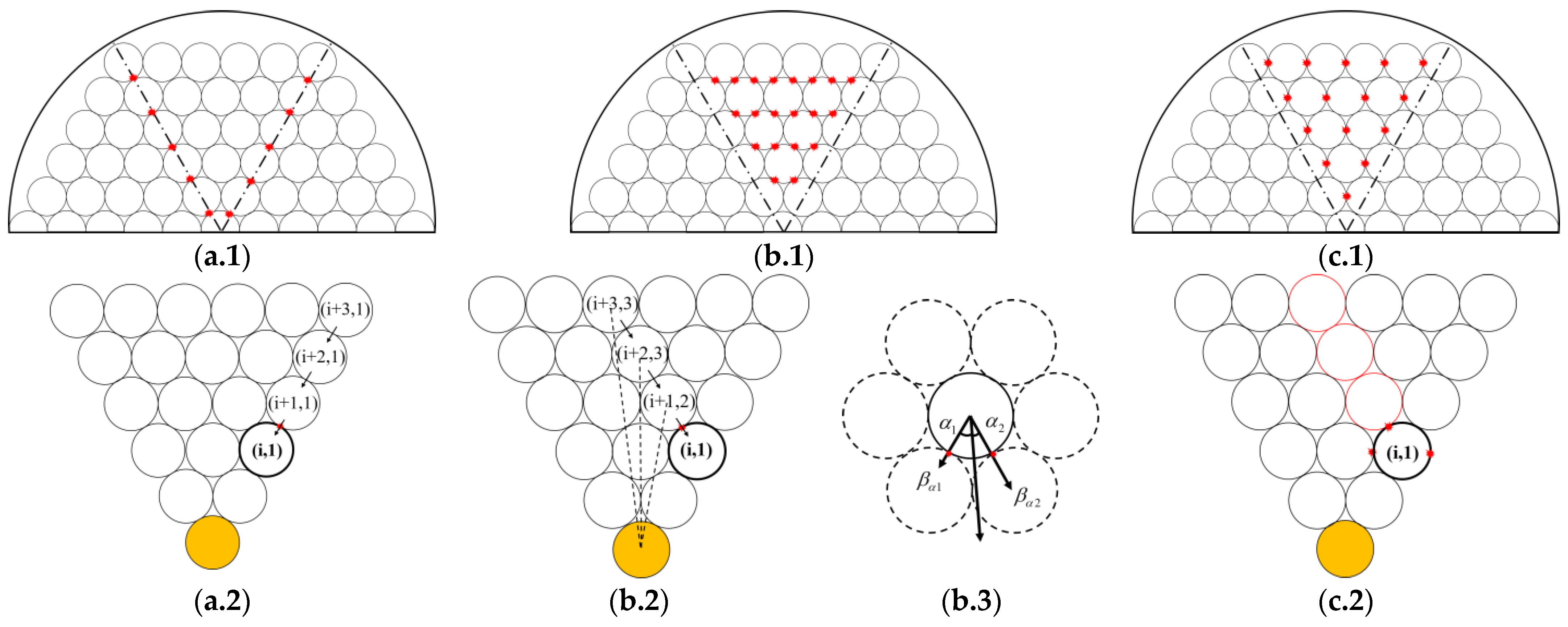
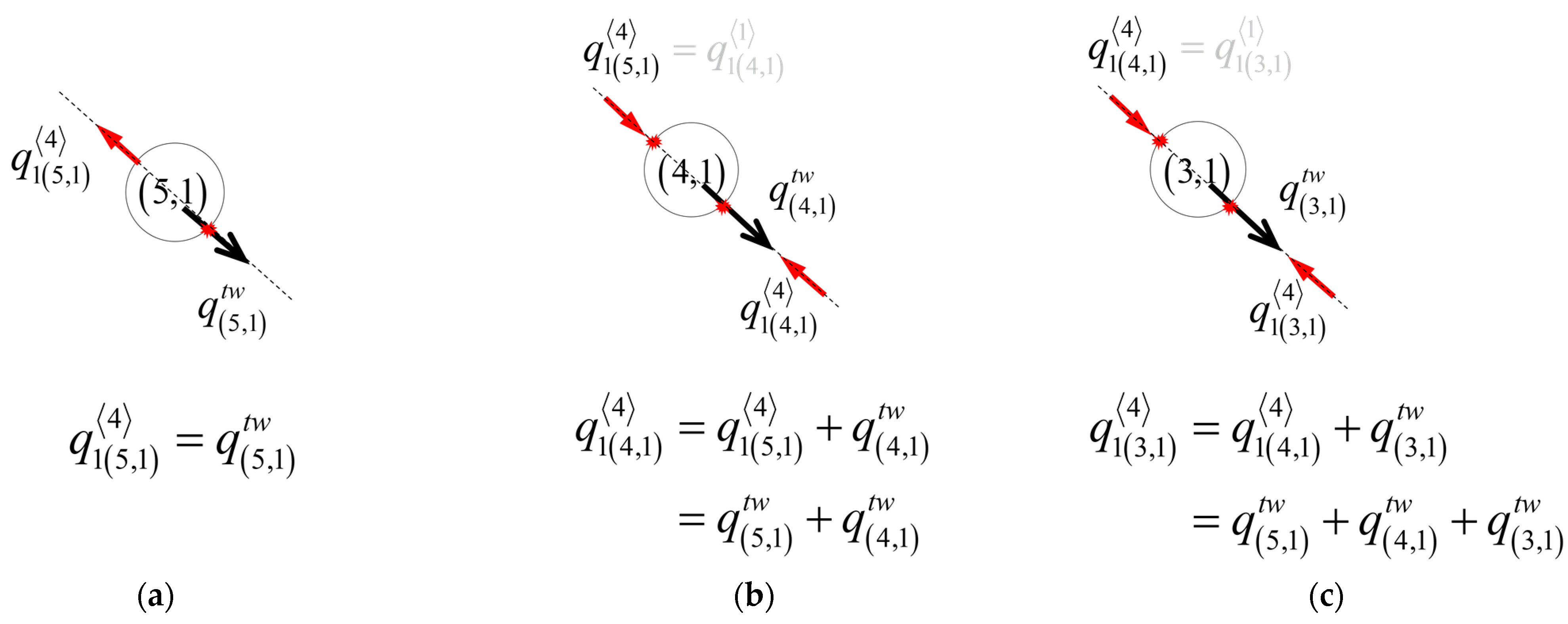
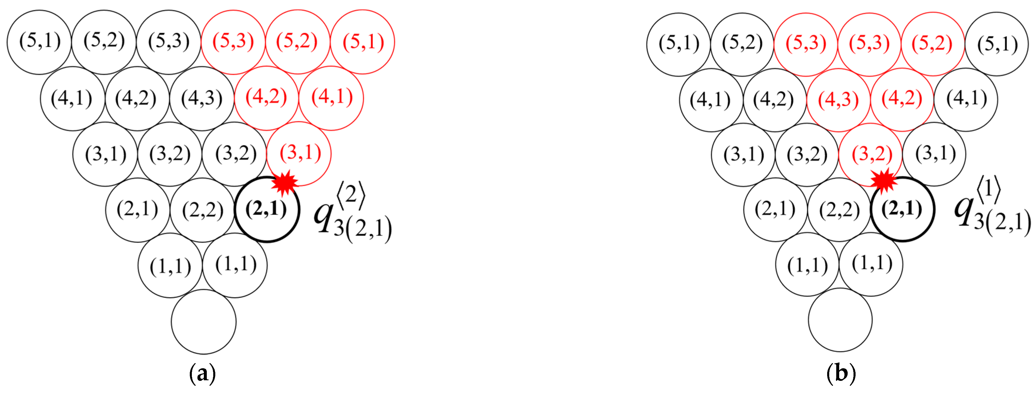
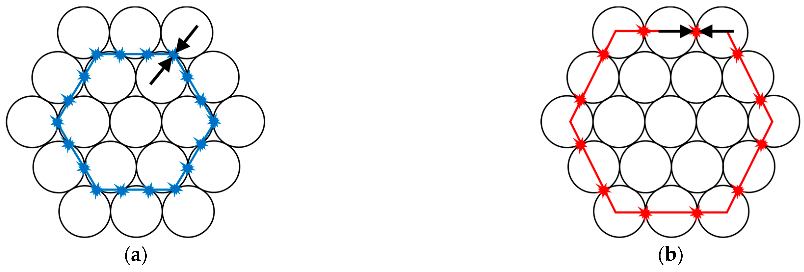
2.2.1. Diagonal Contact Points

If the contact points between the wires are situated along the diagonal of the cable, as Figure 4(a.2) shows, the path for the inward transmission of contact pressure is distinctly clear. All the upper-layer wires transmitting contact pressure are aligned along the line connecting the upper-layer wire to the central wire. The contact pressure generated by twisting can thus be directly transmitted to the calculated contact point and can be directly computed as follows:

$$q_{1\left(i,1\right)}^{\langle k\rangle }={\displaystyle \sum _{l=1}^n{q}_{\left(i+l,1\right)}^{tw}}$$

(2)

where $〈k〉$ represents the position of the contact point on the wire, and can take values 1, 2, 4, and 5.

For instance, in the case of Figure 4(a.1), the calculation of the contact pressure at point $〈2〉$ on the wire $\left(i,1\right)$ involves the superposition of all the contact pressures from the upper-layer wires. This can be expressed as follows:

$$q_{1\left(i,1\right)}^{\langle 2\rangle }=q_{\left(i+1,1\right)}+q_{\left(i+2,1\right)}+q_{\left(i+3,1\right)}$$

(3)

For contact points on different layers of wires, the contact pressure on either side of the same wire is distinct, with the difference being equal to the twisting force exerted by that wire, as shown in Figure 5b by $q_{1\left(\mathrm{5,1}\right)}^{〈4〉}-q_{1\left(\mathrm{5,1}\right)}^{〈1〉}=q_{\left(\mathrm{5,1}\right)}^{tw}$. Conversely, the contact pressure between two adjacent wires at a contact point is identical, as shown in Figure 5b by $q_{1\left(\mathrm{6,1}\right)}^{〈4〉}=q_{1\left(\mathrm{5,1}\right)}^{〈1〉}$.

2.2.2. Non-Diagonal Contact Points in Different Layers

If the contact point between wires is not on the diagonal and is situated between different layers, as shown in Figure 4(b.1–b.3), the inward transmission path of contact pressure becomes more intricate, necessitating individual consideration for each wire’s position. In such cases, the angle between the upper-layer wire and the central wire must be taken into account, and a reduction in the twisting force should be applied before superposition.

$$q_{1\left(i,j\right)}^{\langle k\rangle }={\displaystyle \sum _{l=1}^n{q}_{\left(i+l,j\right)}{\beta }_{\left(i+l,j\right)}}$$

(4)

For example, in the case of Figure 4(b.2), the calculation of the contact pressure at point $〈1〉$ on the wire $\left(i,1\right)$ involves the superposition of all the contact pressures from the upper-layer wires. This can be expressed as follows:

$$q_{1\left(i,1\right)}^{\langle 1\rangle }=q_{\left(i+1,1\right)}{\beta }_{\alpha 2\left(i+1,1\right)}+q_{\left(i+2,1\right)}{\beta }_{\alpha 2\left(i+2,2\right)}+q_{\left(i+3,3\right)}{\beta }_{\alpha 2\left(i+3,3\right)}$$

(5)

where ${\beta }_{\alpha 2}$ is the reduction coefficient in the direction of the angle ${\mathrm{\alpha }}_2$, and it is calculated by the following formula:

$$\begin{array}{l}{\beta }_{\alpha 1}=\frac{\sin {\alpha }_2}{\sin {120}^{\circ }}\\ {\beta }_{\alpha 2}=\frac{\sin {\alpha }_1}{\sin {120}^{\circ }}\end{array}$$

(6)

For contact points between wires on different layers, since the direction of the twisting force is generally not along a straight line with the contact point, it is necessary to consider allocating the twisting force to different contact points based on the angle during superposition.

As Figure 6 shows, the superposition of twisting forces can be demonstrated using wire (5,2), (4,2) and (3,2) as an example. For the outermost wire (5,2), the contact pressure mainly depends on its own twisting force $q_{\left(\mathrm{5,2}\right)}^{tw}$ and reduction coefficient ${\beta }_{\alpha }$. And for the inner wires (4,2) and (3,2), their contact pressure is related to the contact pressure transmitted by the upper wire and its own twisting force at the same time.

2.2.3. Non-Diagonal Contact Points in Same Layer

If the contact point between the wires is not on the diagonal but between two wires of the same layer, it is as shown in Figure 4(c.1,c.2).

According to the principle of force equilibrium, the contact pressure on both sides of the contact points within the same layer of wires is equal. Therefore, the contact pressure between the wires within the same layer will eventually be equal to the interlayer contact pressure between the diagonal wires in the other half of the section (as shown in Figure 7a, where $q_{1\left(\mathrm{4,1}\right)}^{〈3〉}$ is equal to $q_{1\left(\mathrm{4,1}\right)}^{〈6〉}$, and $q_{1\left(\mathrm{4,1}\right)}^{〈6〉}$ can be calculated from $q_{1\left(\mathrm{5,2}\right)}^{〈4〉}$; Figure 7b,c has similar rules of computation). In such cases, the contact pressure between wires within the same layer can be calculated by the following formula:

$$q_{1\left(i,j\right)}^{\langle k\rangle }=q_{1\left(i,1\right)}^{\langle h\rangle }$$

(7)

where $〈k〉$ represents the position of the contact point on the wire, and $k$ can take values 3 and 6; $〈h〉$ represents the contact point with an equal contact pressure between wires within the same layer, and $h$ can take values 1 or 2.

For example, in the case of Figure 7, where the marked contact points have equal contact pressure, one can refer to the case of interlayer contact points and calculate the contact pressure between wires within the same layer.

Through Formulas (2), (4), (7), the contact pressure caused by twisting at the six contact points around a single wire can be calculated.

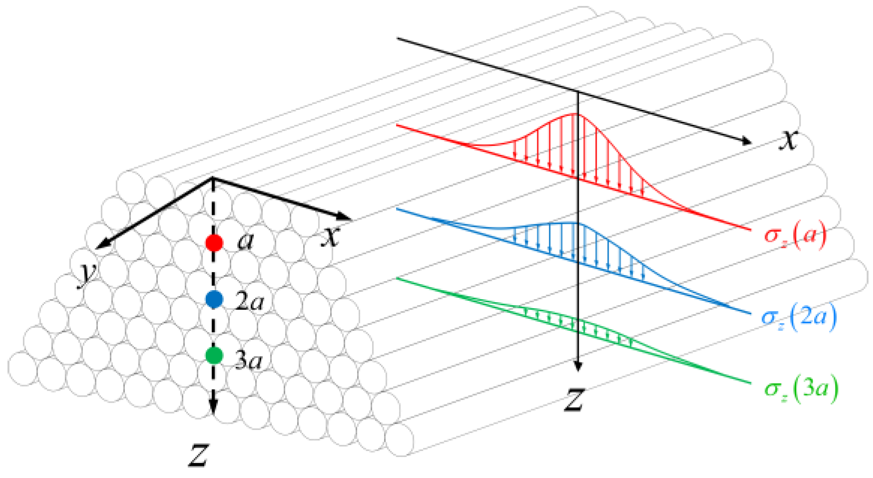
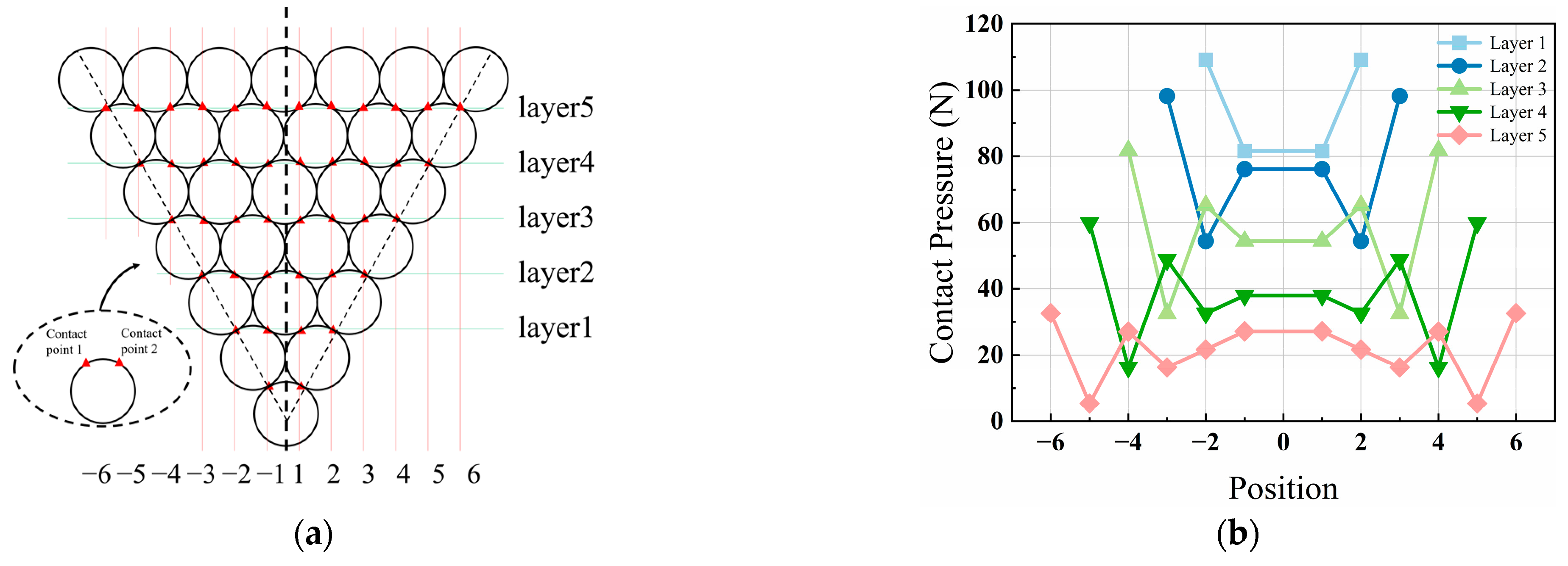
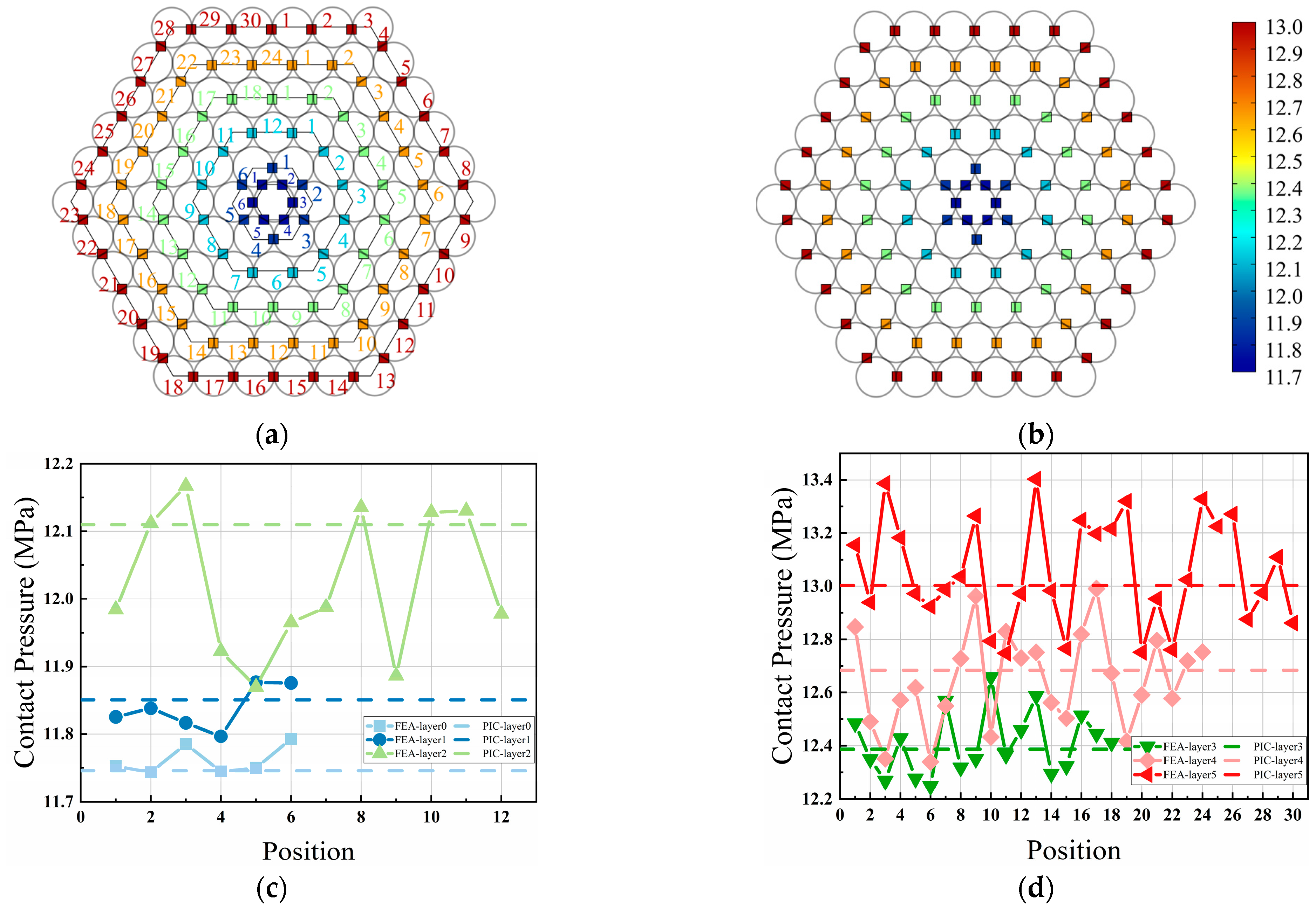
2.3. Contact Pressure Caused by Sheath Compression

An important source of contact pressure between wires arises from the inward radial force generated by the compression of sheaths, fixtures, and the like, causing the internal wires to come into close contact. A complete cross-section of a cable is typically composed of nearly a hundred wires. When in close contact and without slippage, the contact pressure between the wires is transmitted through force chains, following the principles of Boussinesq distribution. As Figure 8 shows, the contact pressure becomes smaller as the depth increases, and the farther away from the place where the load is applied, the smaller the contact pressure. The distribution of contact stress in two-dimensional planes and three-dimensional spaces is related to the magnitude of the external radial force $P_r$, the distance to the outermost sheath $z$, and the longitudinal distance $l$ considered from the position where the load is applied. By integrating the Boussinesq distribution over the longitudinal axis (x-direction), the formula for calculating contact pressure can be obtained:

$$q_2\left(z,l\right)={\displaystyle {\int }_{-l}^l-\frac{2P_r{z}^3}{\pi {\left(x^2+z^2\right)}^2}}dx=P_r\cdot \frac{2}{\pi }\left(\frac{zl}{z^2+l^2}+{\tan }^{-1}\left(\frac{l}{z}\right)\right)$$

(8)

where $P_r$ is the radial force exerted by the HDPE (high-density polypropylene) sheath on the cable, which is the compression force per unit length of the HDPE sheath, considered to be linearly distributed; $z$ is the distance from the contact calculation point to the outermost of the cable cross-section; $l$ is the range considered at the calculation point.

The radial contact force $P_r$ provided by the HDPE sheath is a result of the constriction effect caused by the cold shrinkage $\Delta t$ of the outer extruded high-density polyethylene. The direction of $P_r$ is the direction of the sheath circumference, while the direction of $T_p$ is the direction of the sheath radius. We can use the analysis of thin-walled cylinders in mechanics of materials to obtain the relationship between $P_r$ and $T_p$ by integrating along the circumference of the circle. It can be calculated using the following formula:

$$\begin{array}{l}2T_p={\displaystyle {\int }_0^{\pi }\sin t\cdot P_{r}dl}\\ P_r=\frac{T_p}{r_0}=\frac{\beta \cdot \Delta t\cdot h\cdot E}{r_0}\end{array}$$

(9)

where $T_p$ is the stress of the wire caused by the cold shrinkage of HDPE sheath, which can be calculated by $E·\beta h∆t$, $\beta$ is the volumetric thermal expansion coefficient of high-density polyethylene at room temperature; $\Delta t$ is the temperature change; $h$ is the thickness of the polyethylene sheath; $E$ is the elastic modulus of the polyethylene sheath; $r_0$ is the radius of the sheath.

For parallel wires, there is no need to consider the change in contact pressure between the wires and the sheath due to temperature differences. This is because the expansion coefficient of high-density polyethylene sheath differs significantly from that of parallel wires (typically, high-density polyethylene sheath for bridge cables uses $1\times {10}^{-4}/℃$, while the strands use $1.87\times 5/℃$). As for the expansion pressure generated inside the wires due to temperature differences, the numerical value is relatively small compared to the contact pressure generated by sheath compression, and it does not affect the overall performance of the cable [35]. Therefore, it is not further discussed.

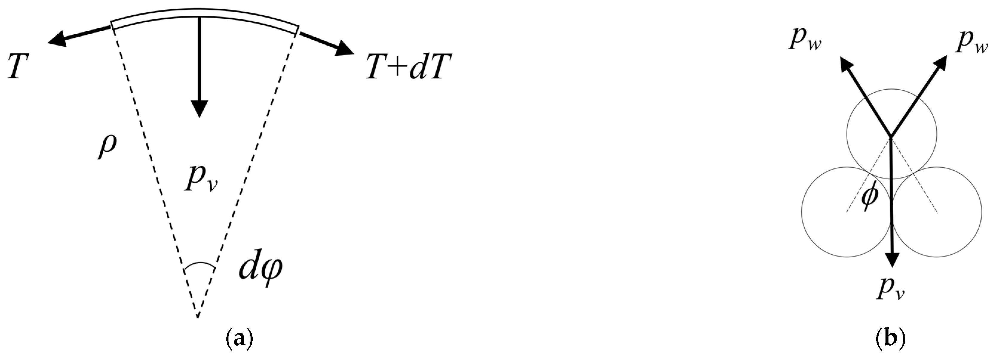
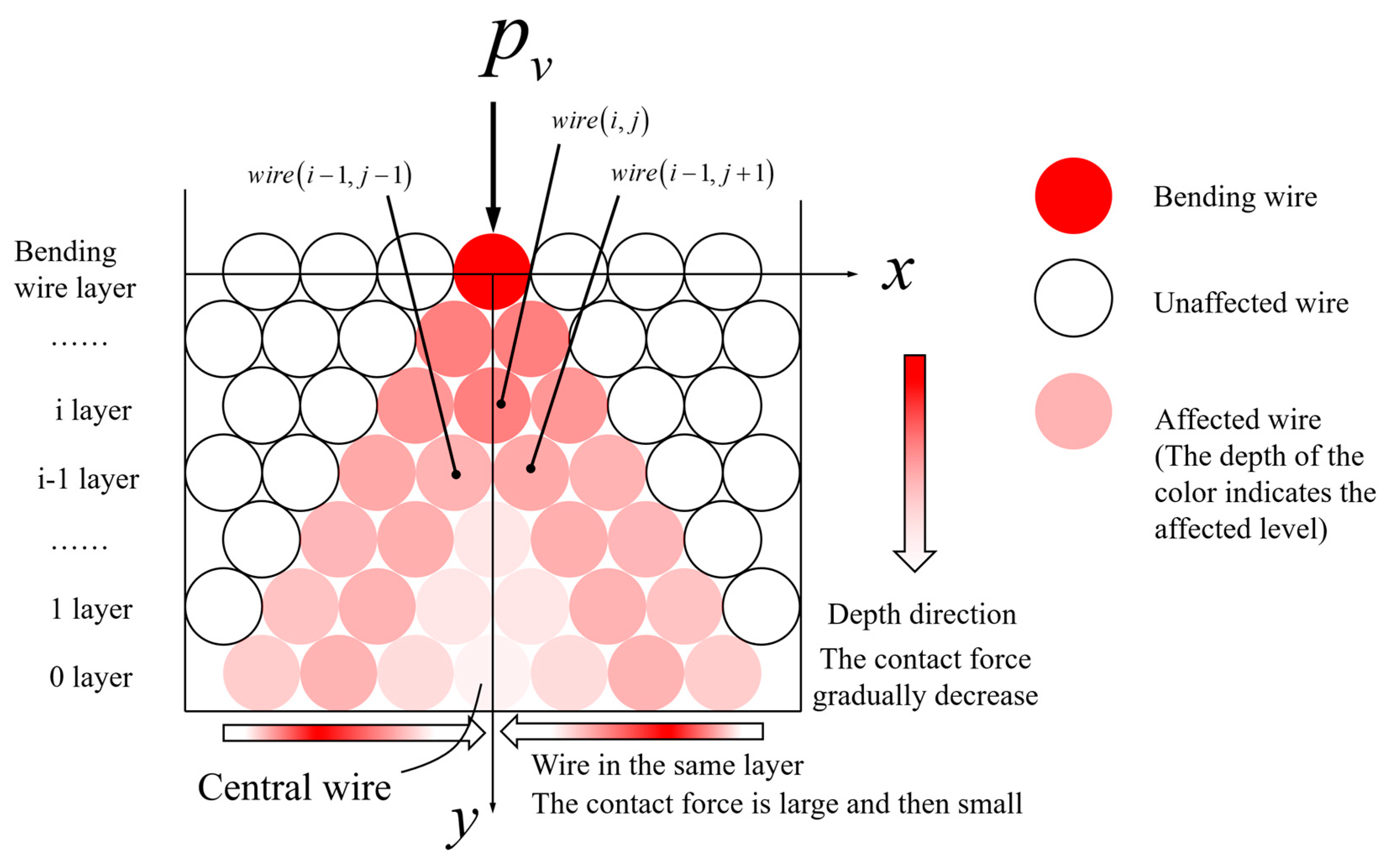
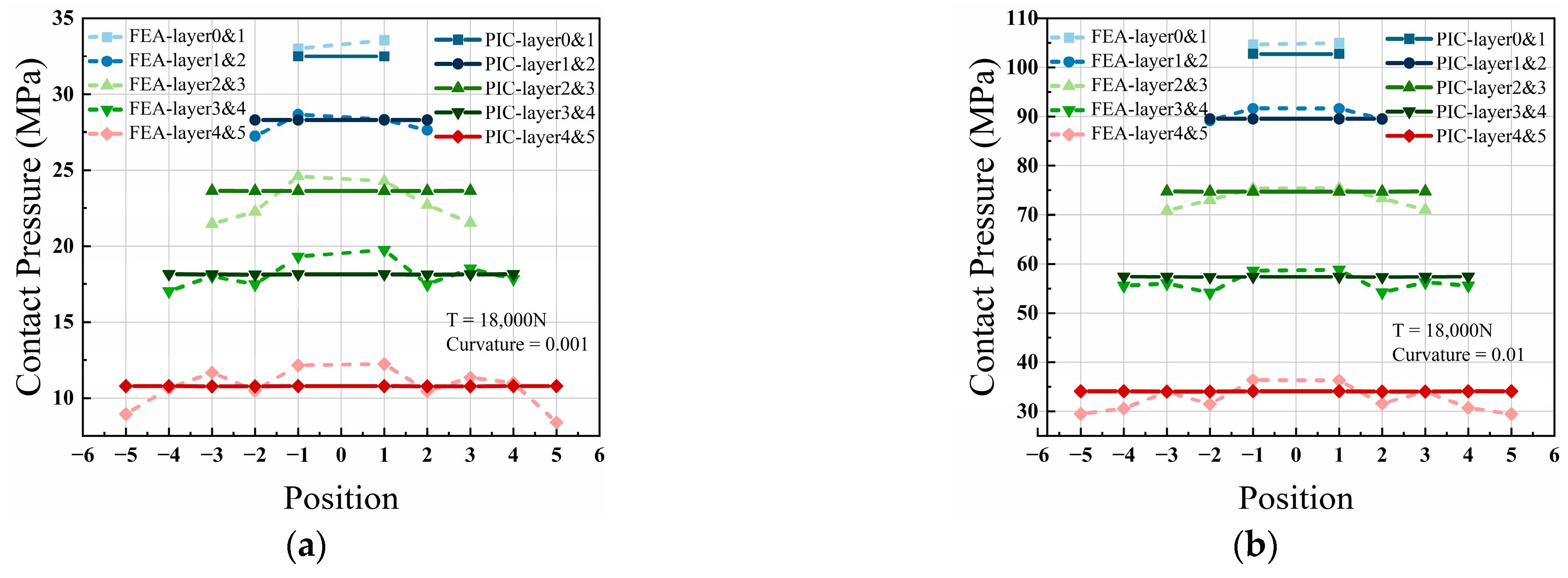
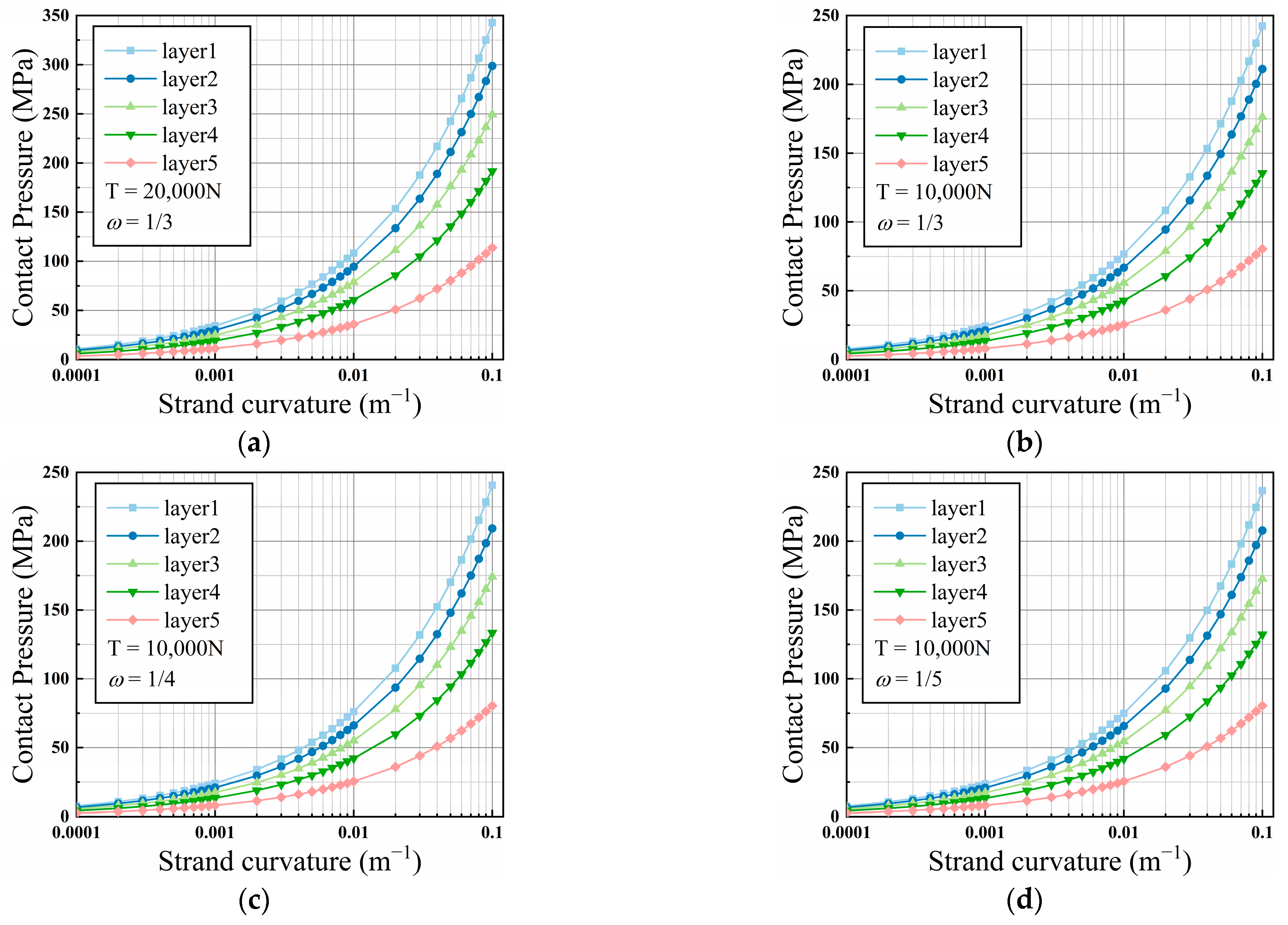
2.4. Contact Pressure Caused by Cable Bending

The third significant source of contact pressure between wires is generated due to the bending of the cables. The cable ends are anchored at the saddle points, and during the vibration process, the cables will experience a certain degree of bending. As individual elements, parallel wires primarily experience tensile stress, and the contact pressure between wires from different layers mainly originates from the vertical radial force of the tensile stress in the wires.

The magnitude of the radial force is related to the tensile force in the wires. As Figure 9 shows, at the contact positions of wires from different layers, the vertical pressure generated by the axial tensile force in the wires is given by:

$$p_v=\frac{2T\sin \left(d\phi /2\right)}{dl}=\frac{2T\sin \left(d\phi /2\right)}{\rho d\phi }=\frac{T}{\rho }$$

(10)

The pressure transmitted from the upper-layer wires to the lower-layer is given by:

$$p_w=\frac{p_v}{2\cos \varphi }=\frac{p_v}{\sqrt{3}}$$

(11)

where $p_v$ is the vertical component of the wire axial tensile force, $p_w$ is the $p_v$ component force transmitted from the upper-layer wires to the lower-layer, $T$ is the tensile force of wires, $\rho$ is the curvature radius of the wire, and $d\phi$ and $dl$ are the angle of bending and the length of the wire.

This type of wire transmission has an accumulative nature; the contact pressure from the upper-layer wires is transmitted to the lower-layer and superposed wires. The transmission pattern conforms to the two-dimensional closely arranged contact force transmission model under concentrated force. Research indicates that the location of maximum stress does not always occur at the centerline but progressively expands layer by layer outward. It symmetrically distributes over two layers along the centerline, exhibiting a distinct bimodal phenomenon [36,37].

As Figure 10 shows, a single wire affects the wires in the conical region below it during the bending of cable, while such an effect decreases as one moves towards the inner layers. The PIC model can be used to compute the extent of the influence exerted by the curvature of the wire on other wires in the cable by employing a force transmission model. This calculation can be expressed in terms of the transmission ratio of force and fluctuation momentum of force.

Assuming there exists the following relationship between the transmission ratio of force and the fluctuation momentum of force [36]:

$$\begin{array}{l}{f}_{\left(i-1,j+1\right)}=\frac{1}{2}+{\omega }_{\left(i,j\right)}\\ f_{\left(i-1,j-1\right)}=\frac{1}{2}-{\omega }_{\left(i,j\right)}\end{array}$$

(12)

where ${\omega }_{\left(i,j\right)}$ is the fluctuation momentum of force for the wire $\left(i,j\right)$, $f_{\left(i-1,j-1\right)}$ is the transmission ratio of force from wire $\left(i,j\right)$ to wire $\left(i-1,j-1\right)$, and $f_{\left(i-1,j+1\right)}$ is the transmission ratio of force from wire $\left(i,j\right)$ to wire $\left(i-1,j+1\right)$.

It can be observed that the force transmission ratio is composed of two parts: one part is the average distribution quantity $1/2$, and the other part is the force fluctuation momentum ${\omega }_{\left(i,j\right)}$.

Therefore, the compression exerted by the bending of an individual wire on the lower-layer wires simplifies the contact pressure between different layers of wires as follows:

$$F_{\left(i,j\right)}=F_{\left(i+1,j-1\right)}\cdot \left(\frac{1}{2}+{\omega }_{\left(i+1,j-1\right)}\right)+F_{\left(i+1,j+1\right)}\cdot \left(\frac{1}{2}-{\omega }_{\left(i+1,j+1\right)}\right)$$

(13)

The fluctuation momentum of force will influence the distribution of contact pressure between different layers of cables, thereby affecting the difference in contact pressure between layers. In practical applications, it should be considered in conjunction with values for parameters such as the number of cable layers and wire radius. For example, taking $\mathsf{\omega }=1/3$, we can calculate the distribution ratio for each layer of wire based on the above formula, resulting in its transmission coefficients, which are listed in the

Table 1. Transmission coefficients across different layers.

Layer	x	0	1	2	3	4	5	6
1	y	1.000	——	——	——	——	——	——
2		——	0.500	——	——	——	——	——
3		0.500	——	0.417	——	——	——	——
4		——	0.319	——	0.347	——	——	——
5		0.106	——	0.324	——	0.289	——	——
6		——	0.107	——	0.318	——	0.241	——
7		0.036	——	0.142	——	0.305	——	0.201

below:

During the vibration process, the curvature radius of the wire changes with time, and it can be obtained as follows:

$${\rho }_0\left(x,t\right)=\left|{\frac{\left(1+{\left(\frac{\partial u\left(x,t\right)}{\partial x}\right)}^2\right)}{\frac{{\partial }^{2}u\left(x,t\right)}{{\partial }^{2}x}}}^{3/2}\right|$$

(14)

It can be assumed that the curvature radius of the central wire is the same as the curvature radius of the cable. Therefore, at different positions on the cross-section, the curvature radius of the wire is given by:

$${\rho }_{\left(i,j\right)}={\rho }_0\pm i{D}_w$$

(15)

where ${\rho }_0$ is the curvature radius of the central wire, $i$ is the number of layers of wires, and $D_w$ is the diameter of the wire.

Layer-by-layer superposition leads to the vertical pressure caused by the bending of the wire as follows:

$$p_{v\left(i,j\right)}^{\langle k\rangle }={\displaystyle \sum \frac{T_{\left(a,b\right)}}{{\rho }_0+R}\cdot {\beta }_{\left(c,d\right)}}$$

(16)

Therefore, the contact pressure between wires caused by bending is given by:

$$q_{3\left(i,j\right)}^{\langle k\rangle }=\frac{p_{v\left(i,j\right)}^{\langle k\rangle }}{\sqrt{3}}=\frac{{\displaystyle \sum \frac{T_{\left(a,b\right)}}{{\rho }_0+R}\cdot {\beta }_{\left(c,d\right)}}}{\sqrt{3}}$$

(17)

For example, for wire (2,1) in Figure 11, when calculating the contact pressure at the contact point $〈2〉$, it is necessary to superimpose the contact pressure distribution values contributed by the wires within the upper conical region.

For ease of calculation, let us expand Equation (17) using $q_{3\left(\mathrm{2,1}\right)}^{〈2〉}$ as an example:

$$\begin{array}{cc}{q}_{3\left(2,1\right)}^{\langle 2\rangle }\cdot \sqrt{3}=& \frac{T_{\left(5,1\right)}}{{\rho }_0+5\sqrt{3}r}\cdot {\beta }_{\left(3,1\right)}+\frac{T_{\left(5,2\right)}}{{\rho }_0+5\sqrt{3}r}\cdot {\beta }_{\left(3,2\right)}+\frac{T_{\left(5,3\right)}}{{\rho }_0+5\sqrt{3}r}\cdot {\beta }_{\left(3,3\right)}\\ & +\frac{T_{\left(4,1\right)}}{{\rho }_0+4\sqrt{3}r}\cdot {\beta }_{\left(2,1\right)}+\frac{T_{\left(4,2\right)}}{{\rho }_0+4\sqrt{3}r}\cdot {\beta }_{\left(2,2\right)}\hfill \\ & +\frac{T_{\left(3,1\right)}}{{\rho }_0+3\sqrt{3}r}\cdot {\beta }_{\left(1,1\right)}\hfill \end{array}$$

(18)

By substituting the tensile forces $T$, cable curvature radius ${\rho }_0$, wire radius $r$, and the transmission ratio of force between different wires ${\beta }_{\left(i,j\right)}$ into the equation, the magnitude of the contact pressure can be calculated.

3. Internal Contact Pressure Model Validation

To validate the PIC theoretical model for contact pressure established in the previous chapter, a comparative analysis was conducted between the computational outcomes and finite element simulation results, and the similarity of the law is illustrated by comparing with the experimental results in other studies.

Theoretical validation involves studying and calculating using parallel wires $91\varphi 7$ as the subject. In the model, the length of the cable is 60 m, the weight per unit length is 40 kN/m, the elastic modulus of the wire is taken as 1.97 GPa, Poisson’s ratio is 0.3, the radius of the wire is 3.5 mm, the twist angle is set at 5°, and the friction coefficient is 0.3.

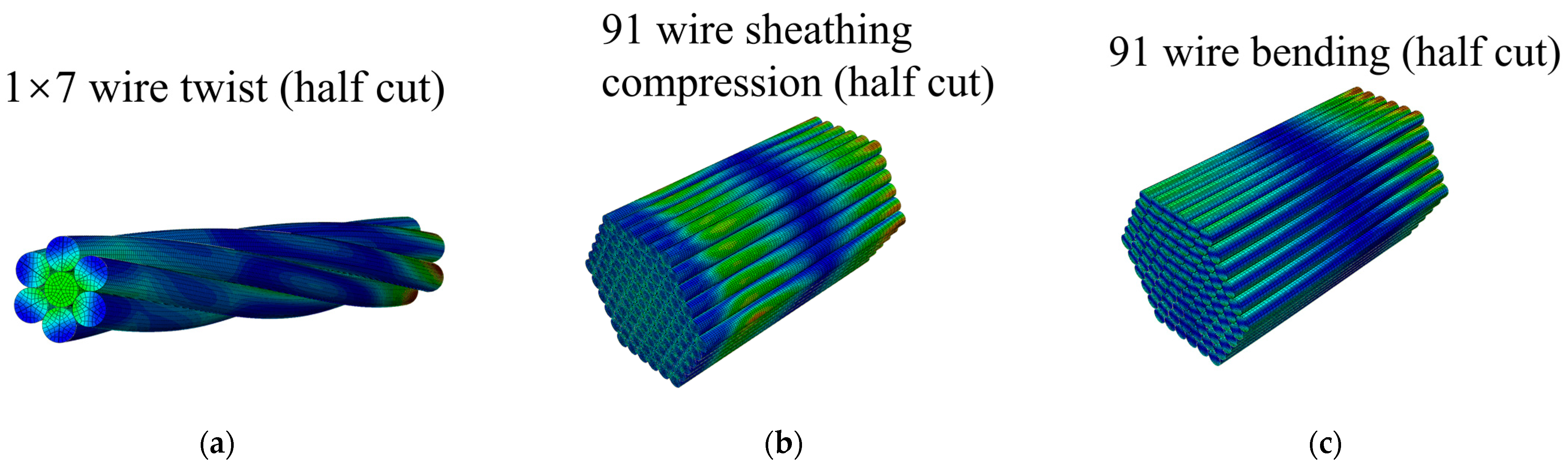
3.1. Formulation of the Finite Element Model

As Figure 12 shows, according to different sources of contact pressure, the corresponding finite element models is established to investigate the distribution patterns and magnitudes of contact stress under different conditions.

The 1 × 7 wire model is established by generating the wire axis from a helix and then sweeping to create the wire surface. This approach is advantageous as it skips the process of transitioning from parallel to helical, saving computational time. The wire end is coupled to a reference point, and fixed constraints are applied to this reference point to anchor the wire end. In the analysis steps, a U2 displacement is applied to the reference point to simulate the stretching process after helical twisting, allowing the wires to make full contact and generate contact pressure. C3D8R elements are used for meshing, and contact is modeled as a hard contact using a penalty function algorithm.

The model for the radial compression of the 91-wire cable involves closely arranging the wires according to the actual situation, creating multiple layers of wire bundles using the array function. Uniform loads are applied to the outermost surface of the wires to simulate the tightening effect caused by the shrinkage of the HDPE sheath due to temperature reduction. This approach provides better control over the magnitude of radial pressure and allows for a more intuitive comparison with theoretical results. Similar to the previous model, the wire ends are coupled to a reference point, and constraints are applied to simulate the boundary conditions of the wires. C3D8R elements are used for meshing, and contact is modeled as a hard contact using a penalty function algorithm.

The model for the bending of the 91-wire cable involves arranging the wires closely, applying uniform pressure to the top of the outermost wire to ensure full contact and induce bending. This method, simulating the bending contact of the wires, is more prone to convergence and ensures sufficient contact between the wires for analyzing the distribution of contact pressure. The boundary conditions for the cable are the same as in the previous two models.

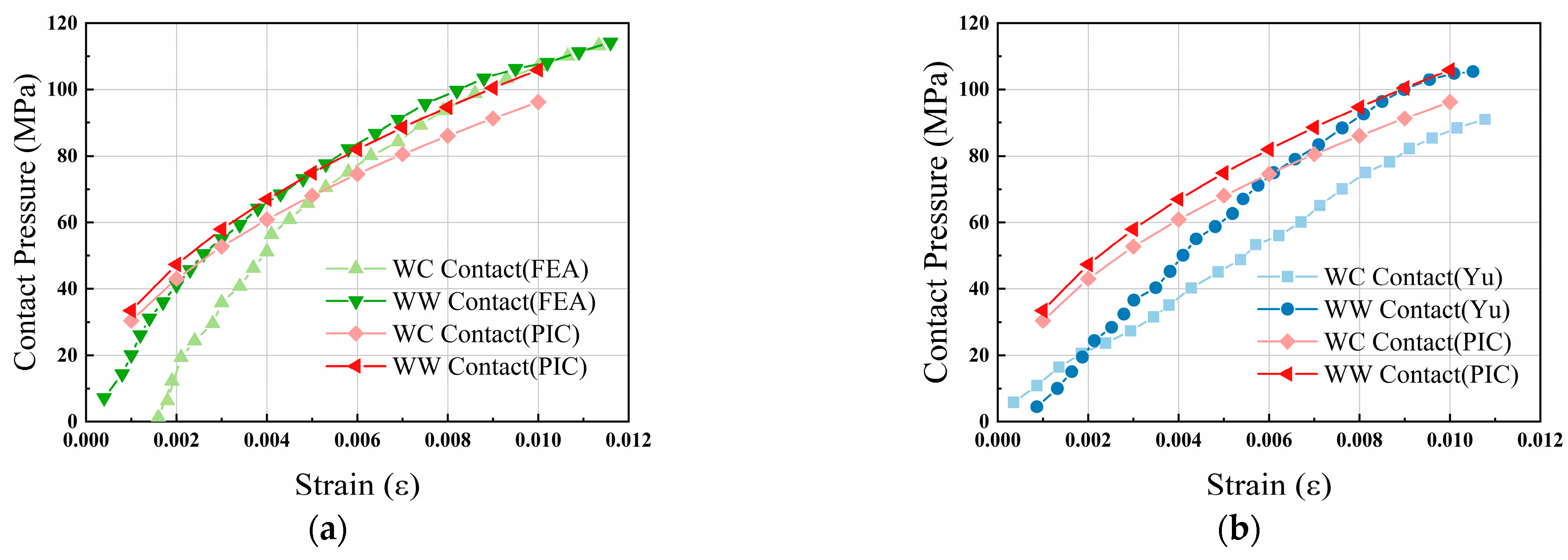
3.2. Validation for Twist Model

The contact pressure caused by twisting in parallel wire cables are smaller compared to that of spiral wires because of the smaller wire twist angle. However, they remain a significant factor that cannot be neglected when calculating contact pressure between the wires.

The 1 × 7 wire model shows that plastic deformation begins to develop when the axial strain in the stay cable reaches 0.006, and the cable enters the plastic zone when the strain reaches 0.01. This study primarily focuses on the development of contact between parallel wires in the elastic zone. Therefore, the contact stress situations within the strain of 0.01 are compared with theoretical analysis.

In the 1 × 7 wire model, the contact includes the contact between the central wire and the helical wire (WC contact) and the contact between helical wires (WW contact). In Yu’s study of the tensile and bending behavior of seven-wire strands [26], a refined model of seven-wire strands was established, and the contact stress patterns between the strands were analyzed. To compare theoretical methods with the results from the finite element model, nodes on the central and helical wires were selected. The relationship between contact stress and wire tensile strain was plotted, and the results were compared with the theoretical approach, the finite element model in this study, and the results from the refined seven-wire model.

As Figure 13 shows, the relationship between the contact stress of wires and tensile strain essentially follows the theoretical model during the elastic phase. Figure 13a illustrates the comparison between FEA (finite element analysis) and the PIC in this study, while Figure 13b illustrates the comparison between FEA in Yu’s paper and PIC in this study. At lower tensile strains, the calculated value of the contact stress is greater than that of the finite element simulation because the torsion force is greater and the contact area is smaller. With increasing strain, the contact relationship between the wires gradually stabilizes, and the stress values obtained through PIC closely align with those of FEA, especially in the elastic phase of the wires, where the conformity is notable. During the elastic phase, the contact stress of WW contact is greater than that of WC contact. This is because at the initial tight contact of the strands, and as the tension is applied, surrounding wires come into contact due to the gripping effect, and consequently, the contact stress in the circumferential direction increases rapidly as tension develops.

As Figure 14 shows, the distribution of contact pressure caused by the twisting of wires is illustrated, with the total cable force computed as 2296.3 kN. Figure 14a shows the hierarchical basis and numbering rules for the contact points of the wires, while Figure 14b shows the distribution of contact pressure between different layers, which generally exhibits an increasing trend toward the inner layers.

Within the same layer, contact points along the diagonal yield the highest contact pressure. This is because contact points along the diagonal lie on the line connecting the upper layer wires and the central wire, facilitating the complete transmission of contact pressure compared to other contact points in the same layer that require reduction. Therefore, these diagonal contact points exhibit a relatively greater pressure. Figure 14c,d shows the distribution patterns of pressure at different contact points, with contact points $〈1〉$ and $〈2〉$ manifesting patterns of monotonically increasing and decreasing pressure, respectively. This behavior is contingent upon the angle between the direction of twisting force and the direction of contact transmission. Due to the twisting forces provided by the upper-layer wires being directed towards the central wire, in the left half-region, contact point $〈1〉$ can accommodate a higher proportion of transmission, while contact point $〈2〉$ experiences fewer transmissions. Conversely, in the right half-region, this scenario is reversed, thereby presenting a distinctly opposite distribution pattern between the two contact points.

Theoretically, the PIC model is also applicable to the calculation of contact pressure between steel wire strands. To validate the efficacy of the theory, the computed results are compared with the contact stress between equally sized steel wire strands [38,39]. Employing an identical configuration of eight layers of wires, a helix angle of 12°, and a wire diameter of 6.5 mm, the comparison is established. As Figure 15 shows, owing to the distinct arrangement of parallel wires and steel strands, the contact pressure in the inner layers (1–4 layers) is significantly influenced by the arrangement. Consequently, the model exhibits substantial deviations from the HDS and MHDS (modified HDS) models. However, in the outer layers (5–8 layers), the errors caused by the arrangement decrease, leading to a more consistent trend between this model and the HDS and MHDS models.

The closer one is to the outer layer of the cables, the smaller the contact pressure, a discrepancy primarily determined by the helix angle ${\mathsf{\alpha }}_{\left(i,j\right)}$ of the wires and the distance $r$ from the central wire. Generally speaking, wires closer to the outer layer exhibit a smaller helix angle and a greater distance from the central axis. According to Formula (1), the calculated contact torsional force is consequently greater, leading to a proportional increase in contact force. Without considering the nonlinear factors, the growth of the contact pressure with strain is linear. Moreover, wires closer to the inner layers experience a higher growth rate. This is because the torsional direction of the wires is directed towards the central wire. The torsional force from the outer layer wires superposes layer by layer onto the contact pressure of the inner layer wires, resulting in greater contact pressure closer to the inner layers, reaching a peak at the central wire. Although the contact pressure of the central wire increases with the addition of wire layers, this growth is not unlimited. For wires in the same layer, the closer to the inner layers, the fewer the contact points, and consequently, there are fewer paths for the transmission of contact pressure. Therefore, the difference in contact pressure between adjacent layers gradually diminishes.

3.3. Validation for Sheathing Compression

Externally enveloped with HDPE sheathing, parallel wire cables are subjected to a radial compression effect caused by the thermal expansion and contraction of the extrusion-molded polyethylene sheath during manufacturing process. Consequently, this compression exerts pressure on the internal wires, leading to their extruded contact and the generation of contact pressure.

The radial compression model for the 91 wires simulates the internal wire-to-wire extrusion caused by the compression of the HDPE sheath on the cables, resulting in the generation of contact pressure. Under the influence of this radial pressure, contact pressure is generated both between different layers of wires, as Figure 16a shows, and within the same layer of wires, as Figure 16b shows. The two types of contact pressure are compared with the finite element model.

Figure 17b,c illustrates the distribution of contact pressure among wires under varying loads for dint layers. Both PIC and FEA exhibit a discernible trend: a diminishing tendency of contact pressure towards the inner layers. The Boussinesq distribution is assumed in the theoretical analysis for the distribution of contact pressure. However, FEA and experimental results deviate from this pattern, possibly attributed to manufacturing errors in the wires during experiments [31]. It is possible that significant disparities in the radius and surface conditions of different wires may lead to an irregular stress distribution. At the same contact position, the greater the external radial force, the greater the contact stress, which is expected. However, in the finite element model, the stress at contact points around the central wire shows a different trend from that of the outer layer wires, which may come from the different distribution of force chains under different loads. Under low loads, there is less deformation induced by wire contact, and internal stresses within the cable mainly transmit along the diagonal of the cross-section. However, under higher loads, significant deformations in internal wires may change the force chain, resulting in certain wires dispersed among the force chains bearing only a fraction of the load [40]. Consequently, the stress distribution changes. On the whole, the PIC model aligns commendably with the actual stress levels between wires. It stands as a convenient method to predict the distribution of internal contact stress in cables, offering preliminary analytical data for experiment and engineering applications.

For the case between the same layer of wire, because the distance between the contact point of the same layer and the central wire is the same, the wire bundle is divided into six layers according to the different distance from the central wire. The comparison of FEA and PIC for contact pressures in each layer is as follows.

As Figure 18 shows, the 0th layer comprises six contact points surrounding the central wire, which exhibit nearly identical contact pressure. However, for layers 1 to 5, there is considerable fluctuation in the contact pressure for the wires within the same layer. This variability arises from the different directions of contact forces among these wires, causing an unstable transmission of force within the same layer. Therefore, the contact pressure between wires in the same layer experiences a greater amplitude of variation compared to wires in different layers. However, there is a clear trend indicating that the contact pressure decreases towards the inner layers. The average contact pressure for the wires within the same layer in FEA aligns closely with the PIC model. This makes the theoretically derived contact pressure an intuitive reference for measuring the pressure levels within the wires.

3.4. Validation for Wire Bending Model

During the vibration of cables, bending occurs, leading to compression between the various layers of wires. As the curvature of the cable increases during the bending process, this compressive effect gradually grows, influencing the contact pressure between the wires.

The model for the bending of the 91-strand configuration involves extracting the contact stress between the wires after the overall curvature of the cable and subsequently comparing it with PIC model. Previous studies show that the interaction forces between the wires exhibit distinct layering characteristics during the process of bending contact [39].

As Figure 19 shows, under different curvatures, both the FEA and PIC reveal a layered pattern in the distribution of contact stress. The contact pressure within the same layer mainly depends on the axial tension in the cable and the curvature, which shows a distinct trend where higher tension and curvature lead to increased contact stress. In PIC model, the force distribution across the cable cross-section is allocated based on its position. As a result, the axial force difference among wires in the same layer is small, resulting in an approximately linear trend in the calculated results. Between different layers, the contact stress increases towards the inner layers, aligning with the assumption of contact pressure accumulating layer by layer. It is noteworthy that wires at positions away from the neutral axis exhibit relatively lower contact stress both in PIC and FEA. This phenomenon may be attributed to the reduced constraint on the outer wires, which may result in inadequate contact between wires and a subsequent decrease in contact force. Additionally, the outer wires are farther from the central wire, resulting in lower axial forces and vertical pressures compared to the inner wires, thus decreasing the available contact pressure for transmission.

Figure 20 illustrates the variation in contact stress and cable curvature under different axial tension levels and force fluctuation coefficients. At lower curvatures, the contact stress induced by bending is almost negligible. However, with an increasing curvature, the contact stress between the wires exhibits exponential growth. Previous studies indicate that the interlayer tangential force in cables also grows exponentially during bending [39]. When the interlayer tangential force surpasses the interlayer frictional force, slippage occurs within that layer. Research on slippage usually assumes equal interlayer frictional forces, but this assumption is inadequate for accurate predictions of wire slippage due to variations in the number of internal wires, friction coefficients, and contact pressure between wires across different layers. Near the neutral axis of the cable, the tangential force between wires is maximal. However, at the same time, the interlayer frictional resistance is also at its peak. Therefore, determining the slippage state requires a consideration of the specific conditions of the cable.

Another crucial factor influencing the interaction forces between wires is the axial tension in the cable. As Figure 20a,b shows, there is a positive correlation between the contact stress among wires and cable tension. It can be inferred that in stay cables with higher tension, the frictional force between the wires is correspondingly greater. This also explains why slippage occurs later in cables with higher tension. The fluctuation in the force between wires affects the difference in contact stress among different layers of wires. A smaller fluctuation in force results in a lesser distribution of force to the inner layers of wires, reducing the loss of contact pressure during transmission and minimizing the difference between layers. If the fluctuation in force is considered a parameter related to the position of the wires, utilizing Markov chain and Taylor series expansion could provide a means to uncover the diffusion pathways of contact pressure among wires within the cable. This approach would offer a more comprehensive understanding of the slippage dynamics between wires.

4. Fretting Wear Analysis Considering Internal Contact Pressure

In order to investigate the influence of contact pressure on fretting wear, the PIC method is employed to calculate the contact pressure between the wires, combined with FEA for the analysis of fretting wear in the wires. Fretting wear is correlated with the conditions of the contact interface, contact pressure, and slip distance. In the analysis process, it is assumed that the conditions of the contact interface remain constant, and the slip distance is accumulated through multiple reciprocating movements.

4.1. Archard Wearing Model

Employing the Archard wear theory to compute the wear depth at each node on the wire contact interface, the equation for the Archard sliding wear can be expressed as follows:

$$\frac{V}{S}=K\frac{F}{H}$$

(19)

where $V$ is the aggregate wear volume, $S$ is the total sliding distance, $F$ is the applied normal force, $K$ is the Archard wear coefficient, and $H$ is the material’s hardness.

For each contact interface, the consideration of wear depth is approached in a differential form:

$$\frac{dV}{dS}=K\frac{dF}{H}$$

(20)

Simultaneously, dividing by $dA$:

$$\frac{dV}{dAdS}=K\frac{dF}{HdA}$$

(21)

In the equation, $\frac{dV}{dA}$ can be replaced with wear depth $d{h}_w$, $\frac{dF}{dA}$ can be substituted with contact pressure $p\left(x,y\right)$, and $\frac{K}{H}$ is a constant, which can be represented as the local wear coefficient. Consequently, the above formula can be expressed as follows:

$$d{h}_w=kp\left(x,y\right)dS$$

(22)

Thus, the equation for the total wear depth is derived:

$$h_w=k{\displaystyle {\int }_0^{n_t}p\left(x,y\right)\delta \left(n\right)dn}$$

(23)

In the equation, $n_t$ represents the total wear cycles, and $\delta \left(n\right)$ denotes the localized sliding distance for the nth cycle.

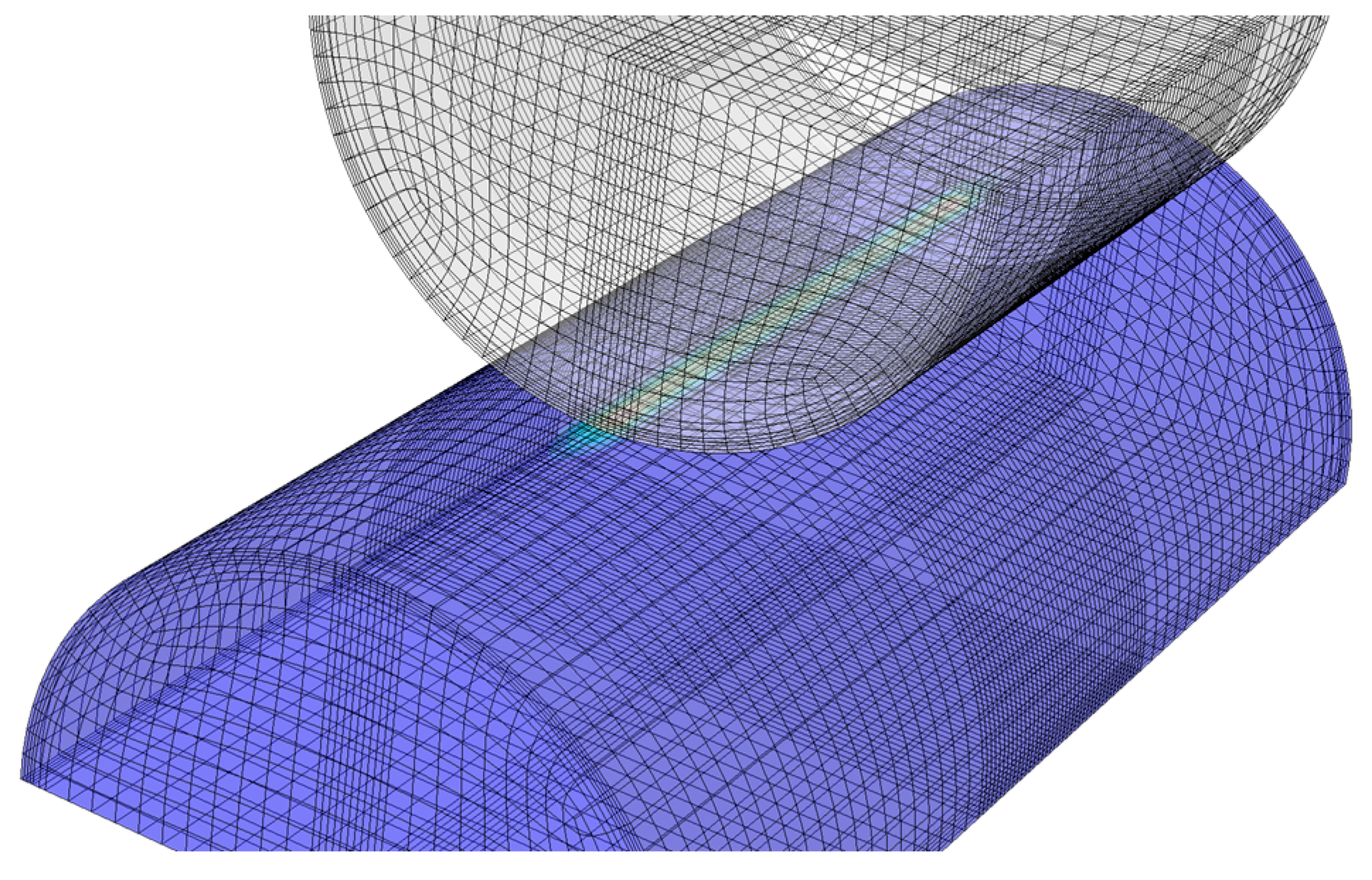
4.2. Finite Element Model of Fretting Wear

The wear model is established with reference to the Archard equation [18], and based on the contact characteristics of parallel wires, reciprocating relative displacements of two semi-cylinders is used to simulate the fretting wear. As Figure 21 shows, the contact wear model of two wires is established in ABAQUS 6.10., and relevant parameters are provided in the

Table 2. Fretting wear coefficient.

Wire radius $R$	$\mathrm{m}\mathrm{m}$	3.5
Young modulus $E$	$\mathrm{G}\mathrm{P}\mathrm{a}$	210
Poisson’s ratio $\upsilon$		0.3
Positive pressure $F$	$\mathrm{N}$	50	100	200
Wear coefficient $k$	${\mathrm{M}\mathrm{P}\mathrm{a}}^{-1}$	8.2 × 10−8
Wire displacement $s$	$\mathsf{\mu }\mathrm{m}$	100
Cycle number $N_t$		100~700

below.

The process of fretting wear fundamentally involves the formation and evolution of wear debris. The contact surfaces undergo continuous sliding friction, leading to adhesion and plastic deformation, accompanied by work hardening to make the material more brittle. In this process, the white layer formed undergoes disruption, peeling, and detachment during reciprocating motion, resulting in the loss of material at the contact interface [3]. Neglecting the influence of wear debris on the fretting wear process, the wear coefficient can be employed to quantify the rate of material loss during this process, enabling the computation of the wear depth at each point on the contact interface. Finite element model is effective in simulating the development of contact parameters during the wear process, providing relevant parameters for fretting wear in the assessment of the service life of stay cable.

Based on the contact model of two wires, this study has developed a finite element subroutine that facilitates real-time updates of node coordinates and interface conditions, enabling an accurate analysis of the wear process. In the finite element software, geometric parameters, material properties, normal loads, and contact characteristics are defined. The subroutine takes input parameters such as sliding distance, total cycle count, and wear coefficient. After completing the calculations, the exported variables CPRESS, CSLIP, and DEPTH can be used to accurately calculate the contact stress and wear depth.

4.3. Result and Discussion

As described in the Archard formula, the wear depth $h_w$ is related to the wear coefficient $k$, contact pressure $P$, total cycle count $\Delta N$, and sliding distance $s$. Integrating Equation (23), the cumulative wear depth can be expressed as follows:

$$h_w=k{\displaystyle \sum _{N_t}P\cdot s}\cdot \Delta N$$

(24)

Under the established conditions of contact pressure and sliding distance, the interface wear depth is directly proportional to the cycle count. In the analysis, this equation can be employed to exert numerical control on the calculation of wear depth.

To gain a deeper understanding of the morphological evolution of the worn surface, Figure 22a and Figure 22b, respectively, show the development of the wear interface and the variation in wear depth at different cycle counts. In order to maintain stable contact at the interface, the FEA does not account for the periodic variation in positive pressure during wire bending. Instead, positive pressure is controlled at 50 N, 100 N, and 200 N, facilitating the calculation of the wear condition at a specific contact point on the wire. It is not difficult to discern that wear depth and cycle count exhibit a positive correlation, and the overall wear rate demonstrates a progressively slowing trend. This phenomenon is attributed to the increasing contact area as wear develops, leading to a gradual “averaging” of wear effects at the contact interface. Consequently, the development of wear depth at various points gradually decelerates, as shown in Figure 22c,d.

Figure 22c shows the variation in interface contact pressure with an applied load of 100 N as the cycle count increases. The peak contact pressure occurs at the center of the contact width. As the contact width increases during the wear process, the peak contact pressure decreases continuously, with the reduction becoming progressively smaller. It is expected that with the development of wear, the contact pressure distribution across the interface will become more uniform, resulting in minimal further changes to the numerical values. According to the Archard theory, under constant wear coefficient $k$, cycle count $\Delta N$, and sliding distance $s$, the development of wear is primarily related to contact pressure. Therefore, the reduction in contact pressure disparity at different positions is the main reason for the “averaging” of interface wear.

Figure 22d shows the variation in contact width with an increasing cycle count under loads of 50 N, 100 N, and 200 N. Under these three loads, the contact width gradually increases with an increasing cycle count, aligning with the results calculated using Hertz’s formula. The contact width experiences rapid growth in the initial few hundred sliding cycles, while the growth trend notably slows down after 500 cycles, consistent with the earlier analysis of contact area.

The wear progression rate is primarily determined by contact pressure. Therefore, regions farther from the contact center exhibit slower wear progression and a smaller increase in contact width. The impact of load on the growth of contact width is significant. A higher load results in a larger contact width under the same cycle count. However, it is important to note that such positive correlation is not unlimited. The marginal effect of the load on contact width is evident, and excessively high loads can change the contact mode from gross slip to partial slip, complicating the wear analysis.

5. Conclusions

In this study, the contact pressure between parallel wires in the stay cable is classified into three types based on their sources: contact pressure caused by wire twisting, contact pressure caused by sheath compression, and contact pressure caused by cable bending. Theoretical derivation and finite element analysis of contact pressure calculation at the six contact points around an individual wire are conducted. A comparison with relevant existing research is performed to validate the effectiveness of PIC model. Finally, based on the theoretical derivation results and considering the influence of loads and cycle counts, a simulation analysis of fretting wear between two wires is conducted. The main conclusions are as follows.

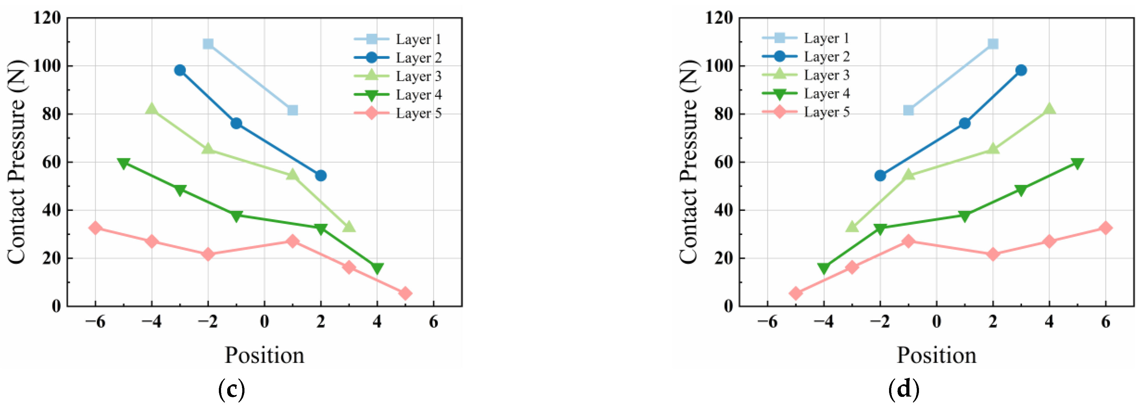
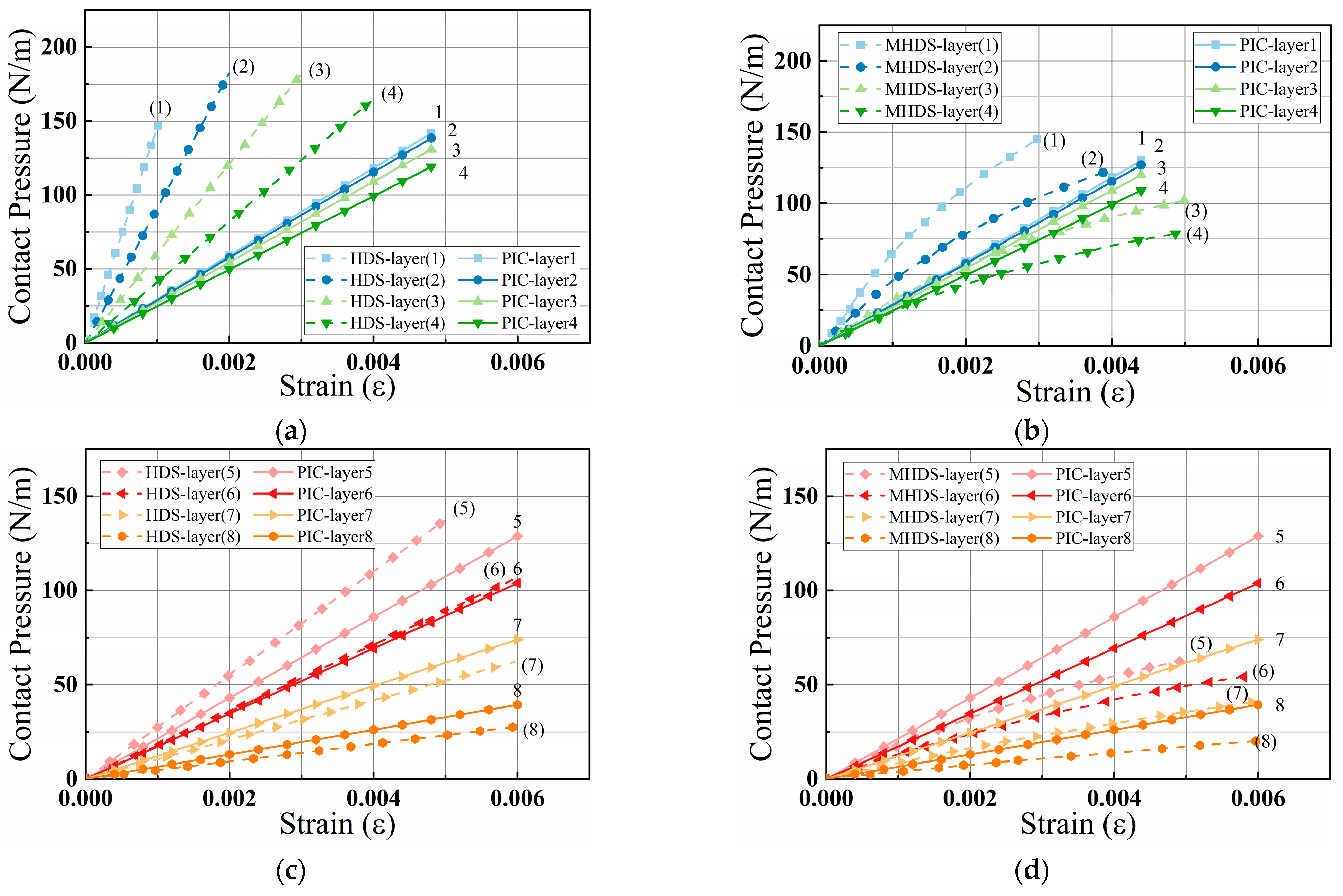
• For parallel wires, although the helix angle is relatively small, the contact pressure caused by twisting is still significant. Due to the different axial tension and twist angle, the magnitude of the contact pressure from twisting provided to the inner wire is mainly related to the position of the outer wire. The transmission of contact pressure has a cumulative effect, resulting in greater contact pressure for wires closer to the inner side. Within the same layer, the contact pressure is maximized at the points along the diagonal.
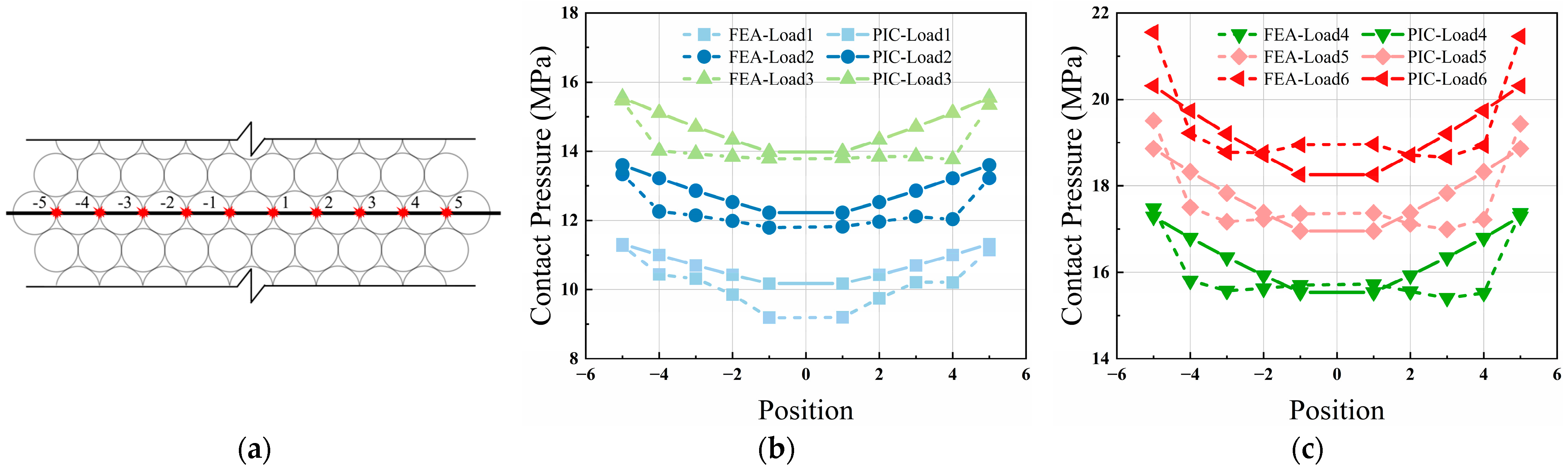
• The distribution of contact pressure between wires caused by sheath temperature shrinkage can be calculated according to the Boussinesq distribution. This assumption is reasonable when not considering variations in force chains caused by manufacturing errors. The results of calculations under this assumption show that the contact pressure between wires exhibits distinct layering, which is consistent with the results of finite element simulations.
• The contact pressure caused by the bending of the wire fluctuates with the variation in wire curvature during the vibration process of the stay cable and is also related to the axial tension of the wire. The cable exhibits distinct layering during the bending process, with relatively minor variations in contact pressure within the same layer. The wire curvature is the most significant factor influencing the contact pressure, showing an exponential relationship between the two. For cables with higher axial tension, the contact pressure is also greater, providing a lateral explanation for the delayed occurrence of slipping in stay cables with higher tensile forces. The location of the initial slipping within the cable cannot be determined to occur at the neutral axis or the outermost layer, owing to the different distributions of tangential force and interlayer frictional resistance within the stay cable.
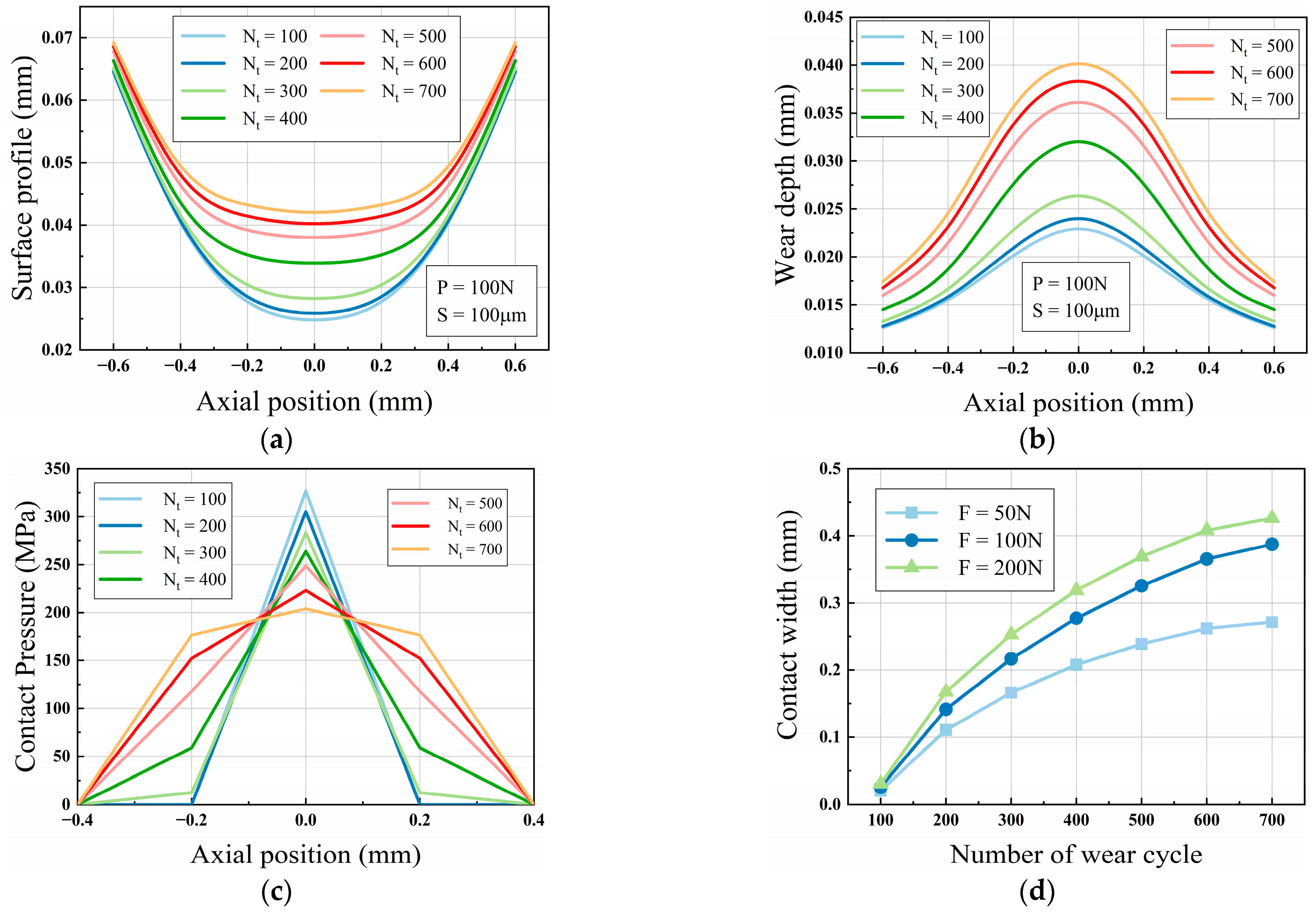
• Based on the existing calculation results, fretting wear between two wires was simulated in finite element analysis. According to Archard’s theory of wear, it is possible to make certain estimations regarding the development of wear depth. Finite element analysis indicates that with an increase in cycle count, wear at the contact interface gradually becomes more uniform. The main reason for the averaging effect is the reduction in the disparity of contact pressure at various points. In addition, the width of the contact area at the interface increases in proportion to the increase in contact pressure. However, such an increase is not unlimited, as excessively high contact loads can change the contact mode from gross slip to partial slip, which complicates the wear analysis.

References

1. Zhang, H.; Xie, X.; Zhao, J.L. Parametric vibration of carbon fiber reinforced plastic cables with damping effects in long-span cable-stayed bridges. J. Vib. Control 2011, 17, 2117–2130. [Google Scholar] [CrossRef]
2. Zhuojie, Z. Mechanism and Mechanical Behavior of Delamination and Slippage between Wires or Strands of Cables for Large-Span Bridges; South China University of Technology: Guangzhou, China, 2016. [Google Scholar]
3. Zhou, Z.; Leo, V. Fretting Wear; Science Press: Beijing, China, 2002. [Google Scholar]
4. Cruzado, A.; Hartelt, M.; Wäsche, R.; Urchegui, M.A.; Gómez, X. Fretting wear of thin steel wires. Part 1: Influence of contact pressure. Wear 2010, 268, 1409–1416. [Google Scholar] [CrossRef]
5. Chen, Y.P.; Meng, F.M. Numerical study on wear evolution and mechanical behavior of steel wires based on semi-analytical method. Int. J. Mech. Sci. 2018, 148, 684–697. [Google Scholar] [CrossRef]
6. Zhang, D.; Ge, S.; Zhu, Z. Friction and Wear Performance on Fretting Wear of Steel Wires in Hoisting Ropes. J. China Univ. Min. Technol. 2002, 31, 367–370. [Google Scholar]
7. Zhang, D.; ShiRong, G.E. Research on the contact mechanisms in the process of fretting wear between steel wires. J. Mech. Strength 2007, 29, 148–151. [Google Scholar]
8. Yue, T.Y.; Wahab, M.A. A Review on Fretting Wear Mechanisms, Models and Numerical Analyses. Comput. Mater. Contin. 2019, 59, 405–432. [Google Scholar] [CrossRef]
9. Wang, L.; Shen, R.L.; Zhang, S.H.; Bai, L.H.; Zhen, X.X.; Wang, R.H. Strand element analysis method for interaction between cable and saddle in suspension bridges. Eng. Struct. 2021, 242, 112283. [Google Scholar] [CrossRef]
10. Wang, D.; Zhu, H.; Gao, W.; Zhang, D.; Tan, D.; Zhao, X. Research on Dynamic Contact and Slip Mechanisms of Parallel Steel Wires in the Main Cable of Suspension Bridge. J. Mech. Eng. 2021, 57, 228–242. [Google Scholar]
11. Zhang, H.; Yao, L.J.; Zheng, X.L.; Shen, M.J.; Xie, X. Corrosion-Fatigue Analysis of Wires in Bridge Cables Considering Time-Dependent Electrochemical Corrosion Process. J. Eng. Mech. 2023, 149. [Google Scholar] [CrossRef]
12. Zhongxiang, L. Study on Damage Mechanism and Life Assessment of Bridge Suspenders under Coupled Corrosion-Fretting Fatigue; Southeast University: Nanjing, China, 2019. [Google Scholar]
13. Wang, D.; Zhang, J. Prediction of Fretting Fatigue Crack Propagation Life of Steel Wire Considering Fretting Wear. Tribology 2021, 41, 710–722. [Google Scholar] [CrossRef]
14. Llavori, I.; Zabala, A.; Urchegui, M.A.; Tato, W.; Gómez, X. A coupled crack initiation and propagation numerical procedure for combined fretting wear and fretting fatigue lifetime assessment. Theor. Appl. Fract. Mech. 2019, 101, 294–305. [Google Scholar] [CrossRef]
15. Starkey, W.L.; Cress, H.A. An Analysis of Critical Stresses and Mode of Failure of a Wire Rope. J. Manuf. Sci. Eng. 1959, 81, 307–311. [Google Scholar] [CrossRef]
16. Utting, W.S.; Jones, N. The response of wire rope strands to axial tensile loads—Part II. Comparison of experimental results and theoretical predictions. Int. J. Mech. Sci. 1987, 29, 621–636. [Google Scholar] [CrossRef]
17. Utting, W.S.; Jones, N. The response of wire rope strands to axial tensile loads—Part I. Experimental results and theoretical predictions. Int. J. Mech. Sci. 1987, 29, 605–619. [Google Scholar] [CrossRef]
18. McColl, I.R.; Ding, J.; Leen, S.B. Finite element simulation and experimental validation of fretting wear. Wear 2004, 256, 1114–1127. [Google Scholar] [CrossRef]
19. Ghoreishi, S.R.; Messager, T.; Cartraud, P.; Davies, P. Validity and limitations of linear analytical models for steel wire strands under axial loading, using a 3D FE model. Int. J. Mech. Sci. 2007, 49, 1251–1261. [Google Scholar] [CrossRef]
20. Meng, F.M.; Chen, Y.P.; Du, M.G.; Gong, X.S. Study on effect of inter-wire contact on mechanical performance of wire rope strand based on semi-analytical method. Int. J. Mech. Sci. 2016, 115, 416–427. [Google Scholar] [CrossRef]
21. Chen, Y.P.; Meng, F.M.; Gong, X.S. Full contact analysis of wire rope strand subjected to varying loads based on semi-analytical method. Int. J. Solids Struct. 2017, 117, 51–66. [Google Scholar] [CrossRef]
22. Huang, N.C. Finite extension of an elastic strand with a central core. J. Appl. Mech.-Trans. Asme 1978, 45, 852–858. [Google Scholar] [CrossRef]
23. Gnanavel, B.K.; Parthasarathy, N.S. Effect of interfacial contact forces in radial contact wire strand. Arch. Appl. Mech. 2011, 81, 303–317. [Google Scholar] [CrossRef]
24. Leclair, R.A. Axial response of multilayered strands with compliant layers. J. Eng. Mech.-Asce 1991, 117, 2884–2903. [Google Scholar] [CrossRef]
25. Johansson, L. Numerical Simulation of Contact Pressure Evolution in Fretting. J. Tribol. 1994, 116, 247–254. [Google Scholar] [CrossRef]
26. Yu, Y. Semi-Refined Finite Element Model of Cable and Its Application on Bending Behavior and Wire Break; Tianjin University: Tianjin, China, 2015. [Google Scholar]
27. Waisman, H.; Montoya, A.; Betti, R.; Noyan, I.C. Load Transfer and Recovery Length in Parallel Wires of Suspension Bridge Cables. J. Eng. Mech. 2011, 137, 227–237. [Google Scholar] [CrossRef]
28. Montoya, A.; Waisman, H.; Betti, R. A simplified contact-friction methodology for modeling wire breaks in parallel wire strands. Comput. Struct. 2012, 100, 39–53. [Google Scholar] [CrossRef]
29. Zheng, G.; Li, H. Normal Stress between Steel Wires in the Stay-cable. In Proceedings of the International Conference on Intelligent Structure and Vibration Control (ISVC 2011), Chongqing, China, 14–16 January 2011; pp. 541–546. [Google Scholar]
30. Brügger, A.; Lee, S.Y.; Mills, J.A.A.; Betti, R.; Noyan, I.C. Partitioning of Clamping Strains in a Nineteen Parallel Wire Strand. Exp. Mech. 2017, 57, 921–937. [Google Scholar] [CrossRef]
31. Brügger, A.; Lee, S.Y.; Robinson, J.; Morgantini, M.; Betti, R.; Noyan, I.C. Internal Contact Mechanics of 61-Wire Cable Strands. Exp. Mech. 2022, 62, 1475–1488. [Google Scholar] [CrossRef]
32. Liu, Y.; Xu, J.Q.; Mutoh, Y. Evaluation of fretting wear based on the frictional work and cyclic saturation concepts. Int. J. Mech. Sci. 2008, 50, 897–904. [Google Scholar] [CrossRef]
33. Argatov, I.; Chai, Y.S. Contact Geometry Adaptation in Fretting Wear: A Constructive Review. Front. Mech. Eng. 2020, 6, 51. [Google Scholar] [CrossRef]
34. Yu, Y.; Chen, Z.H.; Liu, H.B. Advanced approaches to calculate recovery length and force redistribution in semi-parallel wire cables with broken wires. Eng. Struct. 2017, 131, 44–56. [Google Scholar] [CrossRef]
35. Sun, G.; Chen, Z.; Liu, Z. Analytical and Experimental Investigation of Thermal Expansion Mechanism of Steel Cables. 2011, 23, 1017–1027. J. Mater. Civ. Eng. [CrossRef]
36. Hongying, J.; Tiande, M.; Jingbu, L.U. A probabilistic model for force transmission in two dimensional granular packs. Chin. J. Geotech. Eng. 2006, 28, 881–885. [Google Scholar]
37. Liu, Y.; Miao, F.; Miao, T. Force distributions in two dimensional granular packs. Chin. J. Geotech. Eng. 2005, 27, 468–473. [Google Scholar]
38. Hong, K.J.; Kiureghian, A.D.; Sackman, J.L. Bending behavior of helically wrapped cables. J. Eng. Mech.-Asce 2005, 131, 500–511. [Google Scholar] [CrossRef]
39. Khan, S.W.; Gencturk, B.; Shahzada, K.; Ullah, A. Bending Behavior of Axially Preloaded Multilayered Spiral Strands. J. Eng. Mech. 2018, 144. [Google Scholar] [CrossRef]
40. Wensrich, C.M.; Kisi, E.H.; Zhang, J.F.; Kirstein, O. Measurement and analysis of the stress distribution during die compaction using neutron diffraction. Granul. Matter 2012, 14, 671–680. [Google Scholar] [CrossRef]
Figure 1. (a) Cable-stayed bridge; (b) stay cable; (c) cable vibrates and bends; (d) contact caused by wire twist; (e) contact caused by the sheath compression; (f) contact caused by cable bending; (g) twisting model; (h) radial compression model; (i) wire bending contact model; (j) contact pressure distribution from wire twist; (k) contact pressure distribution from sheathing compression; (l) contact pressure distribution from wire bending.
Applsci 14 01401 g001
Figure 2. Cross-section of cable and contact point labeling: (a) wire positional labeling, (b) wire contact point labeling.
Applsci 14 01401 g002
Figure 3. Outer wire twisting: (a) the outer cable is strained and twisted, (b) wire helix angle, (c) wire cross-section.
Applsci 14 01401 g003
Figure 4. (a.1) Diagonal contact points; (a.2) superposition law of twisting force along the diagonal; (b.1) non-diagonal contact points in different layers; (b.2) superposition law of twisting force in different layers; (b.3) angle between twisting force and contact point; (c.1) non-diagonal contact points in same layer; (c.2) superposition law of twisting force in the same layer. Orange circle indicate central wire.
Applsci 14 01401 g004
Figure 5. Superposition of contact pressure at diagonal contact points: (a) contact force and twisting force in the (5,1) wire, and q 5,1 t w is the twisting force in (5,1) wire, q 1 5,1 4 is the contact pressure at the contact point 4 in (5,1) wire, (b) contact force and twisting force in (4,1) wire, (c) contact force and twisting force in (3,1) wire. The red arrow indicates the contact force and the black arrow indicates the twisting force of each wire.
Applsci 14 01401 g005
Figure 6. Superposition of contact pressure in different layers: (a) contact force and twisting force in the (5,2) wire, and q 5,2 t w is the twisting force in (5,2) wire, β α 1 is the distribution coefficient of twisting force at contact point, (b) contact force and twisting force in (4,2) wire, (c) contact force and twisting force in (3,2) wire. The red arrow indicates the contact force and the black arrow indicates the twisting force of each wire.
Applsci 14 01401 g006
Figure 7. Superposition of contact pressure in the same layer: (a) contact pressure in fourth layer of the cable, q 4,1 2 and q 4,1 3 are the contact points on both sides of the (4,1) wire, which can be calculated through the contact pressure between (4,1) and (5,2) wires, (b) contact pressure in third layer of the cable, (c) contact pressure in second layer of the cable.
Applsci 14 01401 g007
Figure 8. Boussinesq distribution in the wire rope.
Applsci 14 01401 g008
Figure 9. Vertical force distribution in different layers, (a) the vertical force caused by cable bending. (b) distribution of vertical force on the two wires.
Applsci 14 01401 g009
Figure 10. Contact pressure distribution caused by cable bending.
Applsci 14 01401 g010
Figure 11. Superposition of the contact pressure at the contact point due to bending. (a) Superposition at the 2 contact point for (2,1) wire. (b) Superposition at the 1 contact point for (2,1) wire. The red asterisk indicates the contact point.
Applsci 14 01401 g011
Figure 12. Finite element model under three contact types: (a) 1 × 7 wire twist model; (b) 91-wire radial compression model; (c) 91-wire bending model.
Applsci 14 01401 g012
Figure 13. The contact pressure of wire due to twisting under different strains: (a) FEA and PIC comparison; (b) Yu-FEA and PIC comparison.
Applsci 14 01401 g013
Figure 14. Contact pressure distribution caused by twisting: (a) number of contact points of different layers; (b) the contact pressure caused by twisting; (c) distribution of contact pressure at contact point 1 ; (d) distribution of contact pressure at contact point 2 .
Applsci 14 01401 g014aApplsci 14 01401 g014b
Figure 15. Comparison of PIC theoretical model with HDS and MHDS model: (a) comparison of HDS and PIC for layers 1–4; (b) comparison of MHDS and PIC for layers 1–4; (c) comparison of HDS and PIC for layers 5–8; (d) comparison of MHDS and PIC for layers 5–8. The solid line 1–8 is the curve of PIC model, and the dashed line (1)–(8) is the curve of steel wire rope model.
Applsci 14 01401 g015
Figure 16. Distribution of contact stress caused by radial pressure: (a) the contact points on the blue line are between different layers of wire; (b) the contact points on the red line are between the same layer of wire.
Applsci 14 01401 g016
Figure 17. Distribution of contact stress caused by radial pressure between wires of different layers: (a) numbering of contact points, red asterisks are contact point on the diagonal; (b) comparison between FEA and PIC for layers 1 to 3; (c) comparison between FEA and PIC for layers 4 to 6. Load1–6, respectively represent external radial forces of 145 N/m, 125 N/m, 105 N/m, 85 N/m, 65 N/m, 45 N/m.
Applsci 14 01401 g017
Figure 18. Distribution of contact stress caused by radial force in the circumferential wires of the same layer: (a) contact point number of each layer of wire; (b) PIC result of contact stress at circumferential contact points; (c) comparison between FEA and PIC for layers 0 to 2; (d) comparison between FEA and PIC for layers 3 to 5.
Applsci 14 01401 g018
Figure 19. Comparison of contact stress between wires in different layers: (a) T = 18,000   N and strand curvature = 0.001; (b) T = 18,000   N and strand curvature = 0.01.
Applsci 14 01401 g019
Figure 20. The relationship between contact stress in different layers and the curvature of the wire: (a)   T = 20,000   N , ω = 1 / 3 ; (b) T = 10,000   N , ω = 1 / 3 ; (c) T = 10,000   N , ω = 1 / 4 ; (d) T = 10,000   N , ω = 1 / 5 .
Applsci 14 01401 g020
Figure 21. Finite element model for contact wear between two wires.
Applsci 14 01401 g021
Figure 22. Finite element wear analysis: (a) evolution of contact surface profile; (b) evolution of wear depth; (c) evolution of contact pressure; (d) evolution of contact width.
Applsci 14 01401 g022