Co-Operatively Increasing Smoothing and Mapping Based on Switching Function

Abstract

Collaborative localization is a technique that utilizes the exchange of information between multiple sensors or devices to improve localization accuracy and robustness. It has a wide range of applications in autonomous driving and unmanned aerial vehicles (UAVs). In the field of UAVs, collaborative localization can help UAVs perform autonomous navigation and mission execution in complex environments. However, when GNSS is not available, it becomes challenging to position the UAV swarm relative to each other. This is because the swarm loses its perception and constraint of the position relationship between each member. Consequently, the swarm faces the problem of the serious drift of relative accuracy for an extended period. Furthermore, when the environment is faced with complex obstruction challenges or a camera with low texture scenes, noise can make it more difficult to solve the relative position relationship between drones, and a single UAV may lose positioning capability. To solve these specific problems, this paper studies a swarm co-operative localization method in a GNSS-denied environment with loud noise interference. In this paper, we proposed a method that utilizes a distributed scheme based on an incremental smoothing and mapping (iSAM) algorithm for state estimation. It incorporates new anchor-free topological constraints to prevent positioning failures and significantly improve the system’s robustness. Additionally, a new switching function is applied in front of each factor of the loss function, which adjusts the switches in real time in response to the input information to improve observably the accuracy of the system. A novel co-operative incremental smoothing and mapping (CI-SAM) method is proposed and the method does not require a complete relative position measurement, which reduces the need for vehicle measurement equipment configuration. The effectiveness of the method is verified by simulation.

1. Introduction

The co-operative positioning of UAV swarms involves multiple UAVs achieving the high-precision positioning of themselves and targets through mutual communication and perception. UAV swarm co-operative positioning technology has a wide range of application prospects in military, civil, and scientific research [1,2]. However, UAV swarm co-operative positioning technology is restricted by [3], for example, limited accuracy, limited range, sensitivity to environmental conditions, cost, and so on. In particular, we are more focused on satellite denial scenarios, as GNSS signals may encounter issues with fading, multipath effects, interference, and spoofing, so GNSS is not reliable [4]. In addition, the electromagnetic environment in GNSS-denied scenarios is often complex and noisy [5]. Therefore, we design the algorithm in this paper to reduce the error and accuracy divergence of relative positioning in the environments mentioned above and improve the robustness of the system without increasing the amount of computation.

To address the issue of location divergence in a swarm, we propose that adding ranging information is the most effective approach. Bluetooth and Wi-Fi are not very accurate, while radio-frequency identification (RFID) has a very limited working distance [6]. Therefore, we suggest using UWB due to its high accuracy and ease of deployment, which is well-suited for the scenario we discussed. However, the ranging accuracy of UWB is limited to the decimeter level. To enhance accuracy, we will apply the visual–inertial odometry (VIO) scheme to the algorithm, which can bring the accuracy level close to the centimeter range [7,8,9]. We have conducted simulations to maintain an overall high accuracy level. Moreover, the advantage of UWB is still in the case of anchors so far, and few people discuss the advantages that UWB can provide in collaborative positioning in the case of anchor-free scenarios. This paper clearly explains the advantages of UWB fusion positioning under anchor-free circumstances.

At the algorithmic level, in the latest research based on ranging methods, there are still scholars who are improving the traditional distributed MDS algorithm [10], and semi-definite programming algorithm [11], but they are not suitable for the scenario in this paper. This paper also involves the problem of multi-sensor fusion. In the field of fusion algorithms, filter-based methods have been gradually replaced by graph optimization methods. In this paper, we mainly focus on graph optimization algorithms.

In summary, the main challenge that this paper focuses on of co-operative positioning at this stage is how to further reduce the divergence of the positioning error and suppress the higher error term in time. The new approach proposed in this paper can effectively solve the current challenges. Therefore, the main contributions of this paper are as follows:

• A novel co-operative incremental smoothing and mapping (CI-SAM) algorithm is constructed and the approach of this paper is innovative.
• This algorithm can accurately realize cluster positioning without additional algorithms such as target detection, reduce swarm location divergence, and avoid single-UAV positioning failures, and can be applied to the cluster formation flight of small UAVs to achieve an accurate collaborative localization capability.
• The new method is easily scalable and can be applied to all mainstream VIO systems; as long as the UWB module is accessed, a collaborative localization system with superior performance can be obtained.

The structure of this paper is organized as follows: Section 1 introduces the current problems and challenges from the perspective of application scenarios, and leads to the purpose and innovation of this paper. Section 2 presents the current development of methods. Section 3 first models the problem, and then introduces the architecture and principles of the algorithms. Section 4 is a simulation comparison of the paper, and Section 5 and Section 6 include our discussions and conclusions.

2. Related Work

2.1. Relative Positioning in GPS/BeiDou Denial

This paper specifically addresses the relative-positioning technology in an environment where GPS/BeiDou signals are unavailable. According to the different measurement objects, it can be categorized into in-cluster measurement and out-of-cluster measurement. Intra-cluster measurement refers to the mutual measurement between UAVs, which can improve the positioning accuracy of the cluster vehicle itself; extra-cluster measurement refers to the measurement of non-co-operative targets by UAVs, which can realize the precise positioning of targets.

Among the techniques for intra-cluster measurements, some scholars have proposed methods for co-operative localization using incomplete measurements. The article in [12] proposes an a posteriori linearized belief propagation (PLBP) algorithm for co-operative localization in wireless sensor networks with nonlinear measurements. The paper in [13] outlines the cooperative localization method and applies it to ultra-wideband (UWB) wireless networks. The authors propose a fully distributed localization algorithm (SPAWN) by mapping a statistically inferred graphical model onto the network topology, resulting in a network factor graph, and developing a suitable network messaging scheme. The article in [10] proposes a cluster localization architecture and relative localization algorithm based on pigeon flock bionics for collaborative work, flexible configuration, and the efficient operation of unmanned clusters. The paper creatively proposes a relative localization method to construct the relative position relationship with the North Line without resorting to extra-cluster information. The article in [14] proposes batch inverse covariance intersection (BICI) and BICI multi-sensor fusion localization methods with interacting multi-models (IMMs), which are based on the batch form of the sequential inverse covariance intersection (SICI) fusion method. It is also demonstrated that BICI is robust. Compared to SICI, BICI-IMM reduces the estimation error variance of the motion model and has less conservatism. The article in [15] describes a complex micro-vehicle swarm control system stabilized by on-board visual relative localization, the core component of which is a novel and efficient black and white pattern detection algorithm. The system aims to validate the possibility of the self-stabilization of a multi-micro-vehicle swarm in the absence of GNSS. However, limitations on constraints of the testing algorithm lead to non-advantageous practicality.

Among the techniques for out-of-cluster measurements, some scholars have proposed methods for co-operative localization using incomplete measurements. For example, the paper in [16] proposes a collaborative smoothing and mapping (C-SAM) method in 2008. The iSAM algorithm is an incremental smoothing and mapping algorithm based on factor graph optimization [17], which can efficiently deal with large-scale nonlinear least-squares problems and is suitable for state estimation in dynamic scenarios [18], but there were two serious problems in the paper [19]. The first one was that the robots shared observations of the environment among themselves and that the robots made measurements among themselves by observing each other, and the article used black and white tessellated lattices with specific shapes to observe each other. The observation was difficult and required a large amount of shared memory. The other was that the initialization of the algorithm was achieved through multiple iterations, in which virtual anchor nodes were introduced and least squares were used to compute offsets and rotations in different local co-ordinate systems, which was computationally intensive and tedious.

2.2. Topological Factor and Switching Function

The scenario for this paper involves a satellite-denial environment without anchor nodes. It is impractical to deploy anchor nodes in some situations, so the UWB localization scenario without anchor nodes should be considered. Feihu Zhang, in [20], proposed a co-operative vehicle–infrastructure localization method based on a factor graph, which utilizes the topological information between vehicles as constraints to improve the localization accuracy and efficiency of vehicles and other targets in the environment. The papers that have also proposed topological factor constraints include [21,22,23], which is also referred to as the symmetric measurement equation (SME) factor, a topological factor intended to make a difference between the sum of all measured distances and the sum of estimated positions. It provides the covariance of this topological information, which is brought to the back-end for optimization.

In paper [24], a robust switchable constraint-based SLAM back-end method for positional maps is proposed which is capable of identifying and rejecting outliers during the optimization process. A later paper, [25], based on this switching function used the same design for satellite factors. For the switching function, some papers have incorporated it into their topological constraints. The paper [26] proposes a co-operative localization method based on mutual ranging and target orientation measurement between aircrafts using the iSAM algorithm for state estimation, adding topological constraints to the loss function to improve accuracy and adding a switching function before each factor of the loss function to adjust the switching in real time in response to the input information in order to improve the robustness of the system.

3. Models and Methods

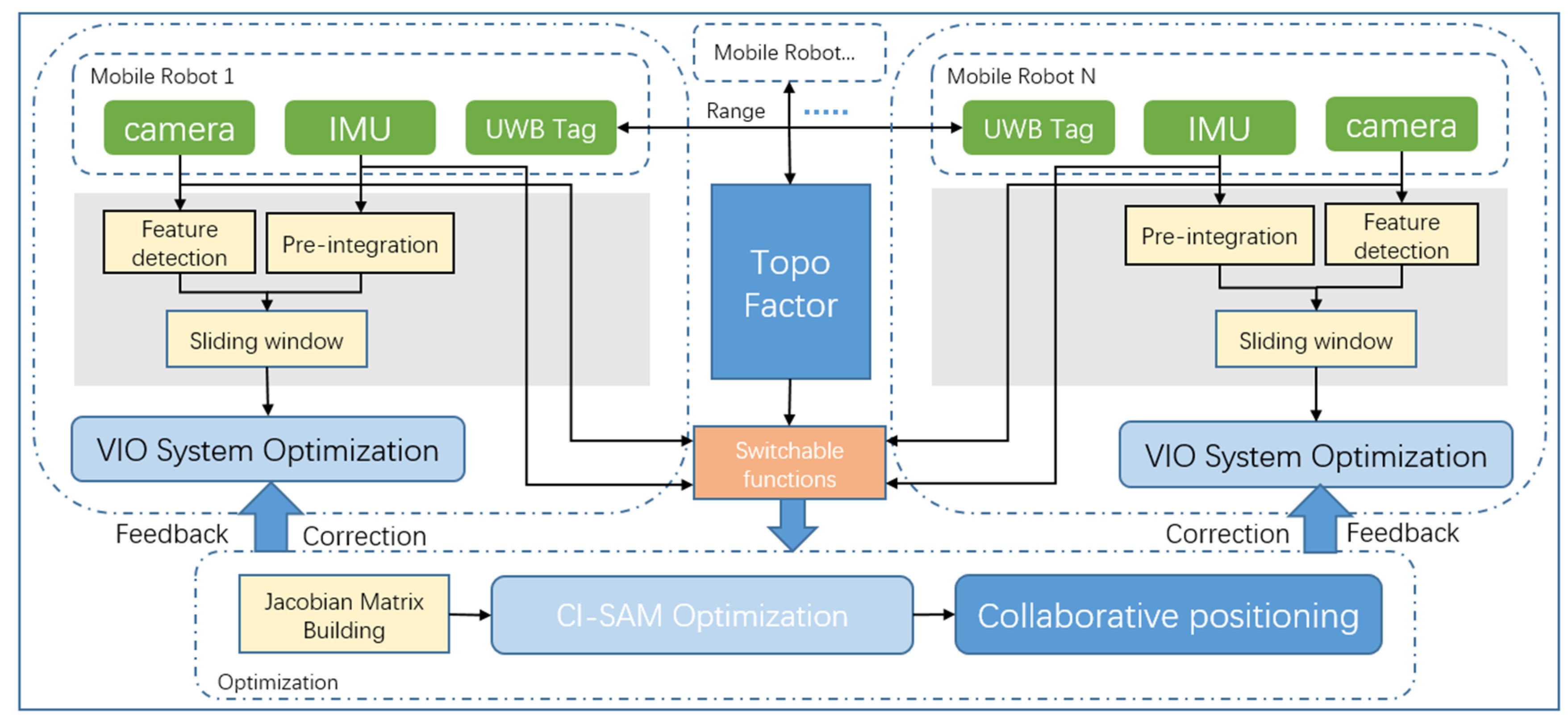
3.1. System Model

The mathematical model and optimization algorithm for collaborative positioning in this paper can be fused using both IMU–camera and UWB sensor data to improve positioning accuracy and robustness. In this paper, we use two types of sensor data for collaborative localization: IMU–camera, which can provide VIO information on UAVs, and UWB, which can provide information on the distance measurement between UAVs. The relative positional relationships between the UAVs are taken into account, which increases the observability and constraints. This paper considers a co-operative positioning system composed of M drones, where the drones can communicate and exchange information with each other. We assume that each drone is equipped with an IMU and a camera, and that the calibration and synchronization between the IMU and the camera have been completed. This paper also assumes that each drone is equipped with a UWB module, and that the calibration and synchronization between the UWB modules have been completed.

We use an optimization algorithm based on graph optimization (GOP) to solve the above mathematical model of collaborative localization. Figure 1 is a block diagram of the algorithm flow in this paper. Graph optimization can represent the optimization variables as nodes in the graph, the constraints as edges in the graph, and the loss function as weights or cost functions on the edges [27]. Graph optimization can utilize techniques such as sparsity, localization, and linearization to reduce computational complexity and memory consumption, and to improve the efficiency and accuracy of a solution.

The loss function for IMU+ camera data represents the consistency constraints between the VIO information of the UAV itself and its position and attitude; i.e., the relative displacements and rotations between two neighboring moments should be equal to the differences in the positions and attitudes under the global co-ordinate system [28]. The loss function for UWB data represents the constraints between the distance measurements between the UAVs and their positions; i.e., the distance measurements between the UAVs should be equal to the modulus of the difference between the positions in the global co-ordinate system.

A simple, basic model is shown above in Figure 2, and, in the scenario of this paper, we use the following qualification: Assuming that the scenario occurs in a two-dimensional co-ordinate system, the vehicle is able to obtain its own a priori position information through GPS or anchor nodes and knows the other nodes’ a priori positions. Each member is initialized with itself as the zero point of the environment co-ordinate system. The ranging information of UWB can be shared among all members. The updating frequency of ranging information is synchronized with the key frame rate of the VIO system. There is no time delay or data error in the communication. The environment has zero clutter, so there is no false detection or omission of the vehicle. Moreover, we do not consider the potential effects of restricted communication between robots and assume that robots have full high-bandwidth connectivity when encountering each other.

The model IMU/UWB/camera problems are as follows:

$$models\left\{\begin{array}{c}{x}_{i,k}=f_k\left(x_{i,k-1},u_{i,k}\right)+w_{i,k}\\ z_{i,k}=h_k\left(x_{i_k},l_{j_k}\right)+v_{i,k}\\ d_{i,j_k}=g_k\left(x_{i_k},x_{j_k}\right)+q_k\end{array}\right.$$

(1)

where $x_{i,k}$ is the state transition equation of IMU itself at time k, and $X=\left\{x_{i,k}\right\}$ with $i\in 0 \dots M$; $l_{j,k}$ is the measurement of the observed landmark point, and $L=\left\{l_{j,k}\right\}$ with$j\in 0 \dots N$; $u_{i,k}$ is the controller input, and $U=\left\{u_{i,k}\right\}$with $i\in 0 \dots M$; and $d_{i,j_k}$ is the UWB measurement from node $i$ to node $j$, and $D=\left\{d_{i,j_k}\right\}$with $i,j\in 0 \dots M$. f, h, and g correspond to their measurement functions. The probability of each node for all parameters and measurements is as follows:

$$P\left(X,L,U,Z,D\right)\propto P\left(x_0\right){{\displaystyle \prod }}_{\alpha =1}^{M}P\left(x_{\alpha }|x_{\alpha -1},u_{\alpha }\right){{\displaystyle \prod }}_{\beta =1}^{N}P\left(z_{\beta }|x_{i_{\beta }},l_{j_{\beta }}\right) {{\displaystyle \prod }}_{\gamma =1}^{K}P\left(d_{i,j_{\gamma }}|x_{i_{\gamma }},x_{j_{\gamma }}\right)$$

(2)

The MAP estimation of $X^{*},L^{*}$ is obtained by minimizing the negative logarithm of the joint probability, which is the linear problem we want to solve:

$$X^{*},L^{*}=arg\underset{X,L}{\mathit{max}}P\left(X,L,U,Z,D\right)=arg\underset{X,L}{\mathit{min}}-logP\left(X,L,U,Z,D\right)$$

(3)

The nonlinear least-squares problem is as follows:

$$\begin{gathered} X^{*},L^{*}=arg\underset{X,L}{\mathit{min}}\left\{{\displaystyle \sum }_{\alpha =1}^M||f_{\alpha }\left(x_{\alpha -1},u_{\alpha }\right)-x_{\alpha }{||}_{{\Lambda }_{\alpha }}^2+{\displaystyle \sum }_{\beta =1}^N||h_{\beta }\left(x_{i_{\beta }},l_{j_{\beta }}\right)-z_{\beta }{||}_{{\Gamma }_{\beta }}^2 \\ +{\displaystyle \sum }_{\gamma =1}^K||g_{\gamma }\left(x_{i_{\gamma }},x_{j_{\gamma }}\right)-d_{i,j_{\gamma }}{||}_{{\Phi }_{\gamma }}^2\right\} \end{gathered}$$

(4)

Linearizing the Equations (5)–(7) yields the following:

$$f_i\left(x_{i-1},u_i\right)-x_i\approx \left\{f_i\left(x_{i-1}^0,u_i\right)+F_i^{i-1}\delta x_{i-1}\right\}-\left\{x_i^0+\delta x_i\right\}=\left\{F_i^{i-1}\delta x_{i-1}-\delta x_i\right\}-a_i$$

(5)

where $F_i^{i-1}$ is the $f_i\left(.\right)$ Jacobian matrix, the expression of which is as follows:

$$F_i^{i-1}:=\frac{\partial f_i\left(x_{i-1},u_i\right)}{\partial x_{i-1}}{|}_{x_{i-1}^0}$$

(6)

$$a_i:=x_i^0-f_i\left(x_{i-1}^0,u_i\right)$$

(7)

The topological constraints for UWB are as follows:

$$\begin{gathered} g_{\gamma }\left(x_{i_{\gamma }},x_{j_{\gamma }}\right)-d_{i,j_{\gamma }}=\left\{g_{\gamma }\left(x_{i_{\gamma }}^0,x_{j_{\gamma }}^0\right)+Q_{\gamma }^{i_{\gamma }}\delta x_{i_{\gamma }}+P_{\gamma }^{j_{\gamma }}\delta x_{i_{\gamma }}\right\}-d_n \\ =\left\{Q_{\gamma }^{i_{\gamma }}\delta x_{i_{\gamma }}+P_{\gamma }^{j_{\gamma }}\delta x_{i_{\gamma }}\right\}-b_n \end{gathered}$$

(8)

$$Q_{\gamma }^{i_{\gamma }}=\frac{\partial g_n\left(x_{i_{\gamma }},x_{j_{\gamma }}\right)}{\partial x_{i_{\gamma }}}{|}_{(x_{i_r}^0,x_{j_r}^0)}$$

(9)

$$P_{\gamma }^{j_{\gamma }}=\frac{\partial g_n\left(x_{i_{\gamma }},x_{j_{\gamma }}\right)}{\partial x_{j{ }_{\gamma }}}{|}_{(x_{i_r}^0,x_{j_r}^0)}$$

(10)

Similarly, for all parameters θ, the linearization result becomes the following:

$$\begin{gathered} \delta {\theta }^{*}=arg\underset{X,L}{\mathit{min}}\left\{{\displaystyle \sum }_{\alpha =1}^M||F_{\alpha }^{\alpha -1}\delta x_{\alpha -1}+G_{\alpha }^{\alpha }\delta x_{\alpha }-a_{\alpha }{||}_{{\Lambda }_{\alpha }}^2+{\displaystyle \sum }_{\beta =1}^N||H_{\beta }^{i_{\beta }}\delta x_{i_{\beta }}+J_{\beta }^{j_{\beta }}\delta l_{j_{\beta }}-c_{\beta }{||}_{{\Gamma }_{\beta }}^2 \\ +{\displaystyle \sum }_{\gamma =1}^K||Q_{\gamma }^{i_{\gamma }}\delta x_{i_{\gamma }}+P_{\gamma }^{j_{\gamma }}\delta x_{i_{\gamma }}-b_n{||}_{{\Phi }_{\gamma }}^2\right\} \end{gathered}$$

(11)

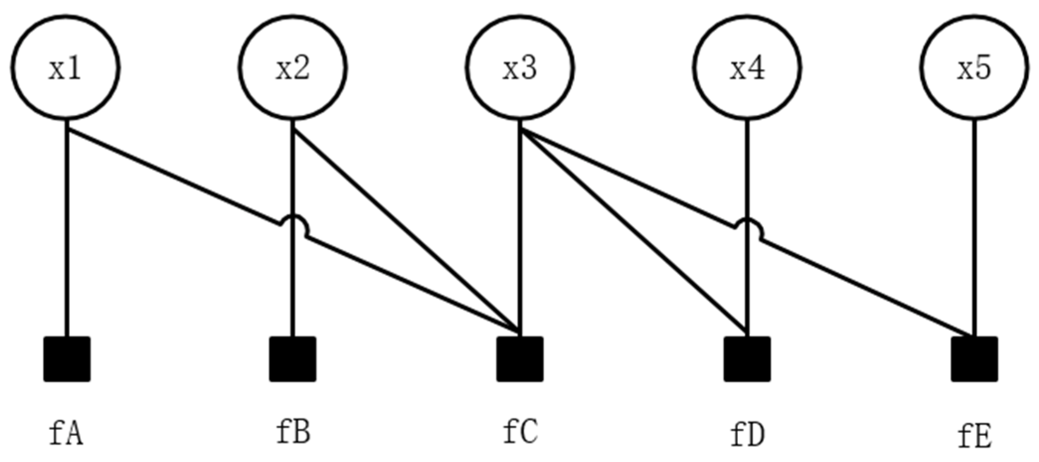
3.2. Factor Graph

A factor graph is a two-way graph used to represent the factorization of a function, which includes variable nodes and factor nodes and represents the relationship between variables and factors through edges. Its advantage is that it can utilize the relative distance information between UAVs to improve positioning accuracy and robustness and reduce the dependence on base stations [28]. In probability theory and its applications, the factor graph is a model that has been widely used in Bayesian inference. The factor graph can model the collaborative localization problem as a probabilistic graph model, where the variable nodes represent the positional states of the UAVs, the factor nodes represent the distance observations between the UAVs or the positional observations of the base station, and the edges represent the associations between the variables and the factors. By performing Bayesian inference on the factor graph, the optimal position estimation of the UAVs can be solved.

The factor graph can flexibly represent multiple types of observations, such as TOA, TDOA, angle, etc., as well as data sources with different accuracies and reliabilities, such as UWB, GPS, vision, etc., so as to improve the accuracy and robustness of the localization. The factor graph can utilize distributed or centralized inference algorithms, such as belief propagation (BP) [12] or maximum a posteriori probability (MAP) [29], to exchange local information among UAVs and achieve globally optimal or suboptimal position estimation. The factor graph can be decomposed or aggregated according to the topology and communication constraints of the UAV swarm, thus reducing the computational complexity and communication overhead and improving the localization efficiency and scalability.

The basic structure of the factor graph is shown in Figure 3. To describe the factor graph model, we assume that the global function is g($x_1, \dots x_n$), where the set {$x_1,\dots x_n$} refers to the variables present in the model. Due to the dichotomous nature of factor graphs, this global function can be expressed as

$$g\left(x_1, \dots x_n\right)={\displaystyle \prod }_{j\in J}{f}_j\left(X_j\right)$$

(12)

where $f_j\left(X_j\right)$ refers to a single factor or function and consists of a subset of variables in {$x_1, \dots x_n$}. To further illustrate this, we can represent this graphically, as shown in the image above, where the variable node is represented by x_n and the factor node is represented by f_n. By turning global functions into maximization problems, ${\mathrm{argmax}}_{X_j}{\displaystyle \prod }_j{f}_j\left(X_j\right)$ is obtained. The optimal solution for the measurement $f_j\left(X_j\right)$ can be found by looking for the right combination of X_j, where X_j represents all known vehicle gestures and landmarks in that factor, maximizing the probability of that particular measurement. Assuming Gaussian noise, linearizing f(x) yields

$$\Delta x^{*}=min||A\Delta x+{b||}^2$$

(13)

where, for $g\left(x\right)=\frac{1}{2}||f\left(x\right)+J^T\left(x\right)\Delta {x||}^2,$ Taylor series expansion is performed, the first-order linear component is retained, the x component is derived, and the value after derivation is 0 to obtain the minimum value of g(x) as $\Delta x^{*}$.

$$J\left(x\right)J^T\left(x\right)\Delta x=-J\left(x\right)f\left(x\right)$$

(14)

For the incremental equation, $H\left(x\right)\Delta x=g\left(x\right)$

$$J\left(x\right)=\frac{\partial f\left(x\left(k\right),l\left(k\right),d\left(k\right)\right)}{\partial x}$$

(15)

Based on the factor graph theory mentioned above, the factor diagram structure of the proposed system is designed, as shown in the Figure 4. The topology can effectively suppress error divergence.

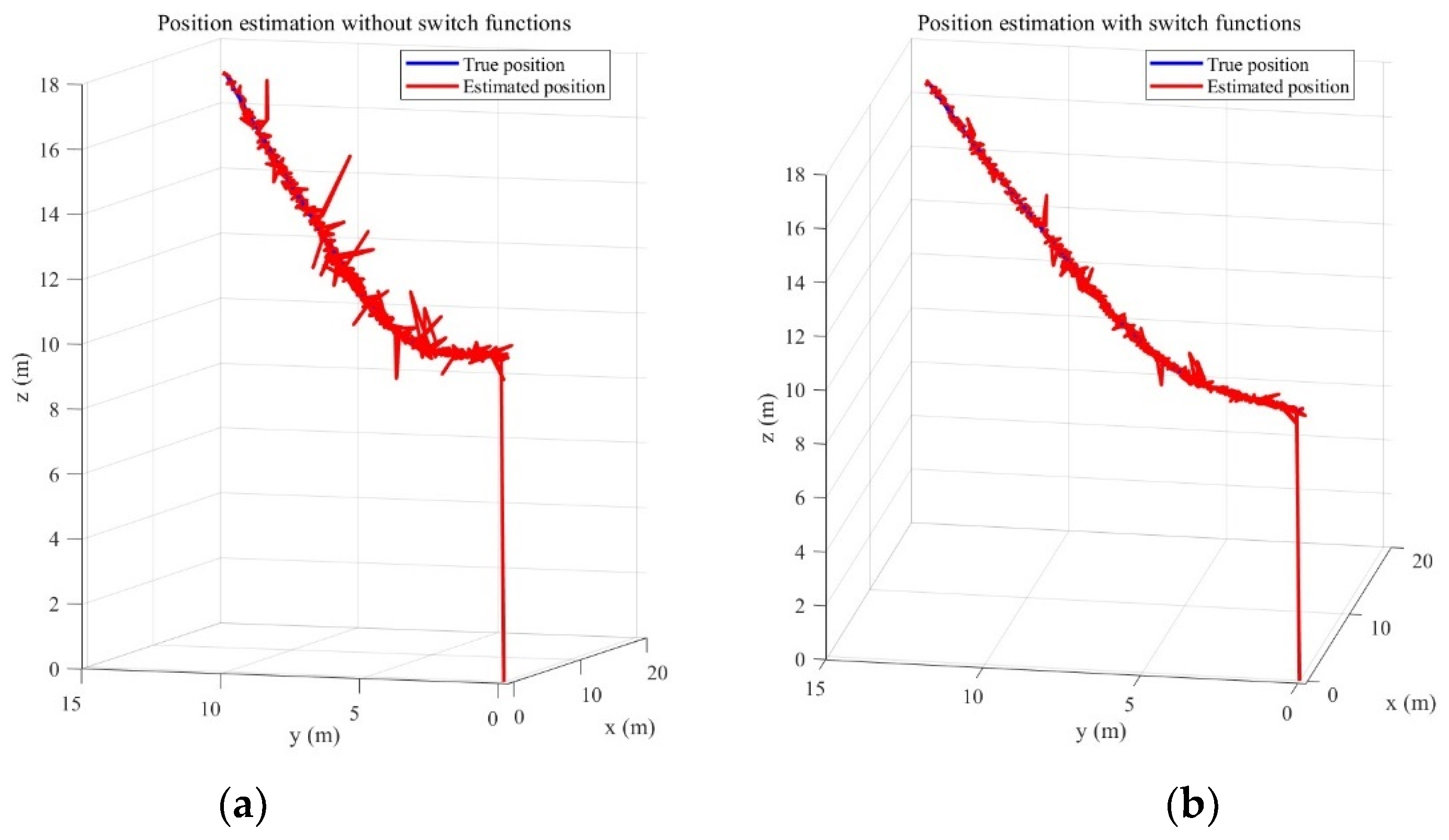
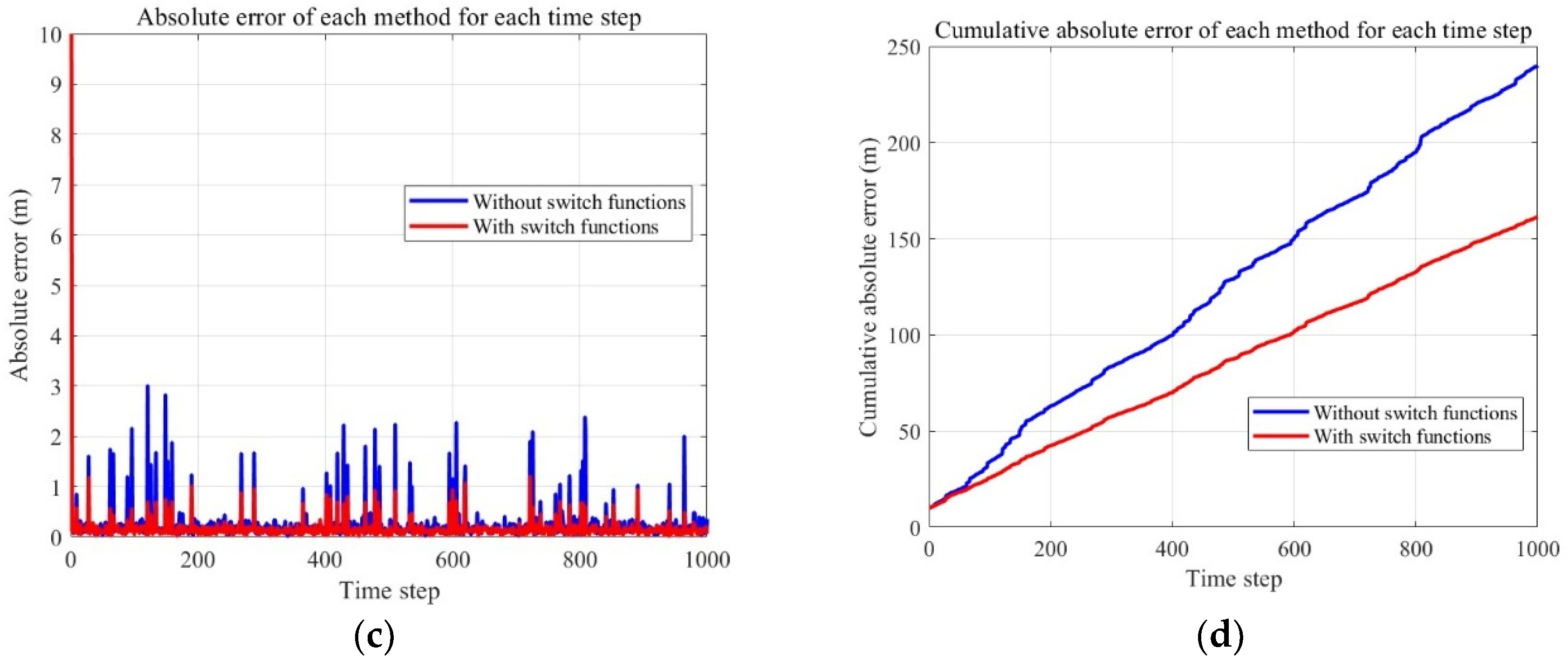
3.3. Switching Functions

A switching function is a function that adjusts the weights of the loss function according to variations and anomalies in the data and suppresses or rejects the effects of anomalies and wild values, thus improving the localization robustness. In this paper, two different types of switching functions are used: one for IMU+ camera data and the other for UWB data. The two types of switching functions have different design and judgment criteria, and the following describes these two types of switching functions, respectively.

IMU–camera data refer to the data provided by the inertial measurement unit (IMU) carried by the UAV itself and the camera, which can form a visual–inertial odometry (VIO) system for estimating the UAV’s position and motion status. The advantage of the VIO system is that it can utilize the visual information from the camera and the inertial information from the IMU for autonomous localization without an external reference, and it can provide high-frequency and low-latency outputs. The disadvantage of the VIO system is that it can cause data anomalies and wild values due to noise, failure, and interference of the IMU and the camera itself, thus affecting the positioning accuracy and robustness. To deal with these problems, this paper describes a switching function to adjust the weights of the loss function of the VIO system.

Two different judgment criteria are used to design the switching function of the VIO system: one is based on the moving speed of the UAV, and the other is based on the consistency of the Mahalanobis distance (MD). The judgment criterion based on the UAV’s moving speed refers to the reliability of the VIO system based on the UAV’s movement state. If the UAV’s moving speed is too fast and exceeds the set threshold, this means that there is a problem with the VIO system and there may be a drift or cumulative error, in which case its weight should be reduced, and vice versa:

$$w_v=\frac{2}{1+e^{k_v\left(v-v_0\right)}}$$

(16)

where w_v is the output value of the switching function, v is the drone’s moving speed, v₀ is threshold, and k_v is coefficient. It can be seen that, when $v\gg v_0$, the switching function w_v is close to zero, which indicates that the VIO system data are unreliable and the weight of the loss function is very small; when v is close to v₀, w_v is close to one, indicating that the VIO system data are reliable and the weight of the loss function is large. In this way, the weight of the VIO system data can be adjusted according to the drone’s moving speed.

The switching function based on MD can judge the reliability of data according to the difference between the data and the prediction value. MD is a distance measure that considers the data distribution and covariance matrix, and it can reflect the correlation and anomaly degree of the data. The larger the MD, the less reliable the data; the smaller the MD, the more reliable the data. This paper uses the following formula to calculate the MD:

$$d_M=\sqrt{{\left(z-\widehat{z}\right)}^T{S}^{-1}\left(z-\widehat{z}\right)}$$

(17)

where z is the observation value, $\widehat{z}$ is the prediction value, and S is the covariance matrix. This paper uses the following formula to calculate the switching function:

$$w=\frac{1}{1+d_M^2}$$

(18)

where w is the output value of the switching function, which represents the weight of the loss function. It can be seen that, when the MD is very large, the switching function is close to zero, indicating that the observation value is unreliable and the weight of the loss function is very small. When the MD is very small, the switching function is close to one; this indicates that the observation value is reliable and the weight of the loss function is very large. In this way, it can effectively suppress or eliminate the influence of outliers and wild values.

This paper uses a switching function to deal with IMU–camera data, which do not participate in the IMU pre-integration process, but only participate in the joint solution process of data fusion. In the joint solution process, this paper uses the following formula to calculate the loss function of IMU–camera data:

$$L_{IC}=w_v·w_{IC}·\left(z_{IC}-h\left(x\right)\right)$$

(19)

where L_IC is the loss function of the VIO system, w_IC is the output value of the switching function, z_IC is the observation value of the VIO system, and h(x) is the prediction value calculated based on the state variable x. In this way, this paper effectively deals with the abnormality and wild values of IMU–camera data.

UWB signals have advantages of high accuracy, low power consumption, and anti-interference, which can provide absolute position information between drones. The advantage of UWB data is that it can perform positioning using distance information without visual information, and it can provide low-frequency and high-accuracy output. The disadvantage of UWB data is that, due to various factors in the signal propagation process, such as obstacles, occlusions, reflections, dynamic objects, etc., it causes phenomena such as signal attenuation, reflection, refraction, multipath, etc., which affect the accuracy and reliability of the data. To deal with these problems, this paper describes a switching function to adjust the weight of the loss function of UWB data.

Moreover, we describe a switching function based on the consistency of UWB data, which judges the reliability of UWB data according to its differences. If there is a large difference in the UWB data, this indicates that there is a problem with the data, which may have noise or outliers, and the weight of the UWB data should be reduced; if UWB data are consistent, this indicates that the UWB data are reliable and the weight should be increased. The following equation is used to compute the switching function based on the movement of the UAV:

$$w_u=e^{-k_u{\left(d_u-d_e\right)}^2}$$

(20)

where w_u is the output value of the switching function, d_u is the sum of distances between UWB data, d_e is the sum of distances calculated based on position estimation, and k_u is the set parameter. It can be seen that, when d_u − d_e is very large, w_u is close to zero, indicating that the UWB data are inconsistent and the weight of the loss function is very small; when d_u − d_e is very small, w_u is close to one, indicating that UWB data are consistent and the weight of the loss function is large. This way, the weight of UWB data can be adjusted according to consistency. In the joint solution process, we use the following formula to calculate the loss function of UWB data:

$$L_{UWB}=w_u·\left(z_{UWB}-h\left(x\right)\right)$$

(21)

where L_UWB is the loss function of UWB data, Z_UWB is the observation value of UWB data, and h(x) is the prediction value calculated based on the state variable x. In this way, this paper can effectively deal with the abnormality and wild values of UWB data. The switching function proposed in this paper can effectively deal with the outliers and wild values of UWB data. The following represents a simulation of the switching function using Python. Assuming that the simulation steps numbered 1000, the switching function had little effect on the simulation results without introducing large errors. Then, random large errors were introduced into the simulation, and the simulation results are shown in Figure 5.

It can be seen from Figure 5a,b that, after adding the switching function, the accuracy was significantly improved when facing random large errors. After multiple tests, the accuracy was improved by about 50% in Figure 5c,d; of course, this was only limited to the introduction of random large errors. If there was always a peaceful and uniform error, the effect improvement was not significant.

3.4. Collaborative Positioning

The first three sections of Section 3 describe the structure of the algorithm and the proposed methodology. The algorithm flow and pseudocode are given in this section. In addition, we will extend the topology constraints to the verification of the positioning results and the relocation of the failed positioning of single UAV. When the new switching functions proposed in the previous chapter are added in the loss function, it becomes

$$\begin{gathered} \delta {\mathsf{\theta }}^{*}=arg\underset{X,L}{\min }\left\{{\displaystyle \sum }_{\alpha =1}^M{w_v}_i^k·{w_{IC}}_i^k·||F_{\alpha }^{\alpha -1}\delta x_{\alpha -1}+G_{\alpha }^{\alpha }\delta x_{\alpha }-a_{\alpha }{||}_{{\mathsf{\Lambda }}_{\alpha }}^2 \\ +{\displaystyle \sum }_{\gamma =1}^K{w_u}_{\mathit{ij}}^k·||Q_{\gamma }^{i_{\gamma }}\delta x_{i_{\gamma }}+P_{\gamma }^{j_{\gamma }}\delta x_{i_{\gamma }}-b_n{||}_{{\mathsf{\Phi }}_{\gamma }}^2\right\} \end{gathered}$$

(22)

where w is the switching function [30]. The above formula adds three different switch factors, which were introduced in detail in the previous chapter. ${w_v}_i^k$ and ${w_{IC}}_i^k$ represent the VIO factor of node i at time k based on the drone’s moving speed switching function and on the MD switching function, respectively. ${w_u}_{ij}^k$ represents the switching function based on the consistency of UWB data between node i and node j at time k. For the VIO factor, the constraint method is used to calculate the following:

$$di{s}_{k,vio}^2=\left[{\displaystyle \sum }_{i=1}^{N-1}{\displaystyle \sum }_{j=i+1}^N{\left(x_{x,k}^i-x_{x,k}^j\right)}^2+{\displaystyle \sum }_{i=1}^{N-1}{\displaystyle \sum }_{j=i+1}^N{\left(x_{y,k}^i-x_{y,k}^j\right)}^2\right]$$

(23)

where $x_{x,k}^i$ and $x_{y,k}^i$ represent the co-ordinates in position obtained by the VIO system i at time k. To obtain the value of the switching function, further calculation of the square of the sum of distances obtained by UWB is required, and, in the same way, $di{s}_{k,uwb}^2 \mathrm{is} \mathrm{obtained}$. In Equation (20), ${\left(d_u-d_e\right)}^2$ is replaced by the following formula:$\left(di{s}_{k,vio}^2-di{s}_{k,uwb}^2\right)$.

It is common for VIO to crash when faced with low feature points and low textures or high-mobility scenes. And, in the experiment, it was found that, when the data of UWB and the data of VIO became unreliable, the positioning results were easy to become confused. In order to further improve the robustness of the algorithm, we will further extend the topological constraints. When the UWB data are unreliable at a certain time, the least two-hop distance between the two nodes or the distance from the previous moment is considered, and the experimental results show that the distance at the previous time has higher accuracy. In addition, when the output result of a single VIO is NAN, we consider the topology of the previous moment and the topology between the drones except the position breakdown one at this moment. According to the improved MDS algorithm, a directionless, centralized co-ordinate after dimension reduction is obtained.

$$B_i=-\frac{1}{2}J{D_i}^{2}J$$

(24)

We suppose n = 3, where D_i refers to UWB measurements matrix at times i, and

$$\left.J=\mathit{E}-n^{-1}\mathit{I}=\left[\begin{array}{ccc}1-\frac{1}{n}& -\frac{1}{n}& -\frac{1}{n}\\ -\frac{1}{n}& 1-\frac{1}{n}& -\frac{1}{n}\\ -\frac{1}{n}& -\frac{1}{n}& 1-\frac{1}{n}\end{array}\right.\right]$$

(25)

is the Eigenvalue decomposition of matrix B_i. Then, B_i becomes

$$B_i=-J{X_i}^T{X}_{i}J=VU{V}^T=V\sqrt{U}{\left(V\sqrt{U}\right)}^T$$

(26)

Then, we have

$$J{X_i}^T=V\sqrt{U}$$

(27)

where $U=diag\left({\lambda }_1,{\lambda }_2\right)$ and $V=\left[q_1,q_2\right]$. Retain the two largest eigenvalues ${\lambda }_1$, ${\lambda }_2$ and corresponding eigenvectors q₁, q₂ to calculate the 2D co-ordinates of the node. According to our previous thought proposed in paper [10], it is possible to convert a problem with 2M degrees of freedom into a problem with 1 degree of freedom, and this only requires the rotation angle to be solved. Then, the rotation angle is found by the least-squares method, and the location of position breakdown UAV is recovered through the topology. After the position is correct, the position and posture of the drone can be corrected through iteration, so as to improve success rate of positioning. This is the improvement for topological constraints. Algorithm 1 summarizes the algorithm to estimate locations of nodes with noisy measurements.

Algorithm 1 Cooperative Increasing SAM Algorithm

Input: IMU_camera_data, UWB_data, GPS_priori;

Output: optimized_nodes_values

1: graph = create_graph()

2: for timestep do in parallel

3:   initialize_nodes_values(graph, GPS_priori)

4:   for each drone do

5:     node = create_node(drone, time_step)

6:     graph.add_node(VIO_node)

7:     Use Equation (19) to calculate the VIO system switching function

8:     graph.add_node(switching_node)

9:   end for

10:   get Topology Matrix D by UWB

11:   graph.add_node(UWB_node)

12:   Use Equation (21) to calculate the topological system switching function

13:   graph.add_node(switching_node)

14:   if single_VIO_position = NAN then

15:     Recovered position by MDS (27)

16:   end if

17:   while(times<max_iterations&&not converged) do

18:     optimize_function(graph)

19:   end while

20:   return optimized_nodes_values

21:end for in parallel

22:return

4. Simulations

To verify the effectiveness and superiority of the proposed method, in this study, we conducted a series of simulation experiments. We used different configurations of drones and different types and degrees of data anomalies and outliers to test the positioning accuracy and robustness of the proposed method under different situations. This paper also compares and discusses other methods to show the advantages and innovations of the proposed method. Simulation experiments refer to experiments that simulate the communication and positioning process between drones on a computer; generate and process sensor data; and obtain and evaluate positioning results. Simulation experiments can conveniently control various parameters and factors, as well as generate various types and degrees of data anomalies and outliers so as to test the method comprehensively and systematically.

This paper was inspired by paper [19], so we compared the results from that paper with the results of this paper, but it is important to note that there is no concept of topological constraints in this paper, and the distances between the aircraft were measured by the camera looking at the pictures of the special shapes carried by the other aircraft. In order to better compare the superiority of the algorithm, we also compare the algorithm error without UWB constraints, and the classic SOTA methods such as UKF and the least-squares method. Both of these two algorithms fuse all observation values, where the error without UWB constraints refers to the result of skipping topology constraint optimization in the proposed algorithm.

This study used five drones to conduct simulation experiments, where the drones communicated and exchanged information with each other. This paper assumes that each drone was equipped with an IMU and a camera, and that the calibration and synchronization between the IMU and the camera were completed. This paper also assumes that each drone was equipped with a UWB module, and that the calibration and synchronization between the UWB modules were completed. The parameters used to set up the simulation experiments are shown in

Table 1. The parameters used in the proposed algorithm are numerical values for experiments.

Parameter	Value	Description
wx	${w_v}_i^k,{w_{IC}}_i^k,{w_u}_{ij}^k$	switching function
${\mathsf{\Phi }}_{\gamma }$	0.2 (m)2	UWB measurement covariance
${\mathsf{\Sigma }}_{UWB}$	1 (m)2	VIO system covariance
${\mathsf{\Sigma }}_{cam}$	0.1 (m)2	camera covariance
${\mathsf{\Sigma }}_{landmark}$	0.2 (m)2/10°	landmark-bearing covariance
${\mathsf{\Sigma }}_{imu}$	0.3 (m)2/5.73°	IMU covariance
${\mathsf{\Sigma }}_{UWB}^{prior}$	0.2 (m)2	UWB measurement prior value
${\mathsf{\Sigma }}_{VIO}^{prior}$	1 (m)2/5.73°	VIO system prior value

.

Experimental dataset: This study used a simulated drone environment with a time of 30 s, which included the flight states of five drones moving away from each other. Each drone was equipped with three types of sensors, IMU, camera, and UWB, and their true positions were recorded as references. Each drone randomly provided IMU, UWB, and camera observations with large errors, simulating the strong interference in a real flight scenario. We used the mean absolute error (MAE) and the positioning success rate (PSR) within 1 m to evaluate the positioning results and compare them with the true values, where PSR means that the algorithm is seriously deviated or has no solution in fifteen similar simulations and MAE refers to the average error after the positioning failure results have been removed.

We conducted four sets of simulation experiments, which tested the influences of different types and degrees of data anomalies and outliers on the method proposed in this paper, in addition to giving a comparison and discussion of other methods. The following are the settings and results for each group of simulation experiments:

4.1. Experiment 1

No anomalies or wild values were introduced. In this study, simulation experiments were conducted without any anomalies or wild values to verify the localization effect of this paper’s method in an ideal situation. The UAV movement time was set to 60 s and the UAV was allowed to move randomly in space. Both IMU+ camera data and UWB data were added with normal levels of noise. An evaluation of the localization results of the various methods is shown in

Table 2. Results of Experiment 1.

Method	Mean Average Error (m)	Positioning Success Rate (%)
IMU–camera only	0.87	80
UKF	0.55	93.3
LS	0.52	86.7
Multi-iSAM [19]	0.44	93.3
CI-SAM (this paper)	0.41	100.0

.

It can be seen from Table 2 that the method proposed in this paper can achieve a high positioning accuracy and precision in the absence of anomalies and outliers. This shows that the method proposed in this paper is effective and superior in ideal situations.

4.2. Experiment 2

IMU–camera data anomalies were introduced. We conducted a simulation experiment in the case of IMU–camera data anomalies to verify the positioning effect of the method proposed in this paper when dealing with IMU–camera data anomalies. The paper set the drone motion time to 60 s and let the drone perform random motions in space. We added a normal level of noise to the IMU–camera data and added outliers at some moments, such as sudden increases or decreases. An evaluation of the localization results of the various methods is shown in

Table 3. Results of Experiment 2.

Method	Mean Average Error (m)	Positioning Success Rate (%)
IMU–camera only	2.13	26.7
UKF	0.83	46.7
LS	0.77	33.3
Multi-iSAM [19]	0.65	66.7
CI-SAM (this paper)	0.42	100.0

.

It can be seen that the method in this paper was still able to maintain a high localization accuracy and precision in the presence of anomalies in the IMU–camera data. This indicates that the method in this paper is effective and robust in terms of dealing with IMU+ camera data anomalies.

4.3. Experiment 3

UWB data anomalies were introduced. We conducted a simulation experiment with cases of UWB data anomalies to verify the positioning effect of the method proposed in this paper when dealing with UWB data anomalies. The drone motion time was set to 60 s, and the drone was allowed to perform random motions in space. We added a normal level of noise to the UWB data and added outliers at some moments, such as sudden increases or decreases. An evaluation of the localization results of the various methods is shown in

Table 4. Results of Experiment 3.

Method	Mean Average Error (m)	Positioning Success Rate (%)
IMU–camera only	0.88	80
UKF	1.38	66.7
LS	1.45	46.7
Multi-iSAM [19]	0.96	66.7
Method in this paper	0.43	100.0

.

It can be seen that the method in this paper can still maintain a high localization accuracy and precision in the presence of anomalies in UWB data. This indicates that the method in this paper is effective and robust in terms of dealing with UWB data anomalies.

4.4. Experiment 4

IMU–camera data and UWB data anomalies were used simultaneously. We conducted a simulation experiment in the case of IMU–camera data and UWB data anomalies simultaneously to verify the positioning effect of the method proposed in this paper when dealing with multiple data anomalies. The drone motion time was set to 30 s and the drone was allowed to perform random motions in space. We added a normal level of noise to both IMU–camera data and UWB data and added outliers at some moments, such as sudden increases or decreases. An evaluation of the localization results of the various methods is shown in

Table 5. Results of Experiment 4.

Method	Mean Average Error (m)	Positioning Success Rate (%)
IMU–camera only	3.35	20
UKF	2.75	46.7
LS	2.15	40
Multi-iSAM [19]	1.44	53.3
Method in this paper	0.83	100.0

.

5. Discussion

Table 5 is the core experiment of this paper, and it compares the errors of several different methods when the IMU and UWB data are abnormal at the same time. The simulation results show that the algorithm proposed in this paper can effectively suppress the impact of large errors and ensure the success rate of positioning. The time complexity of this algorithm is close to the original algorithm, so it is not specifically mentioned in the experimental results. Moreover, it can be seen from Figure 6 and Figure 7 that this paper’s method can still maintain a high localization accuracy and precision in the case of simultaneous anomalies in both IMU+ camera data and UWB data, and this paper’s method outperforms other methods in terms of localization error and the localization success rate. This indicates that the method in this paper is effective and robust in dealing with multiple data anomalies, and can effectively utilize multimodal collaboration information to suppress the influence of wild values.

6. Conclusions

This paper proposes a collaborative localization method based on the fusion of IMU–camera and UWB data, which can use the co-operation information between drones to improve the localization accuracy and robustness. We designed a switching function to deal with the outliers and wild values of the IMU–camera data and UWB data, thus suppressing or eliminating their influence. Furthermore, a series of simulation experiments were conducted to verify the effectiveness and superiority of the proposed method.

Our study also has the following shortcomings and directions for improvement: This paper assumes that each drone is in a two-dimensional plane, and further innovative calculations can be made for three-dimensional space in the future. In addition, we used a switching function based on MD to deal with IMU–camera data outliers and a switching function based on the distance sum to deal with UWB data outliers, which may have required more memory consumption and communication bandwidth. Moreover, a graph optimization algorithm based on the Gauss–Newton method was used to solve the collaborative localization problem, which may have required more iteration time and convergence time.

Future work can be improved and extended as follows: The use of different types and configurations of sensors, such as lidar, can be considered in order to increase the diversity and reliability of the data. Different types and configurations of communication modules can be used to reduce the cost and complexity of communication. Finally, the use of different types and forms of switching functions, such as Kalman filters, particle filters, neural networks, etc., can be considered in order to improve the detection and processing ability of data outliers and wild values.

References

- Awasthi, S.; Fernandez-Cortizas, M.; Reining, C.; Arias-Perez, P.; Luna, M.A.; Perez-Saura, D.; Roidl, M.; Gramse, N.; Klokowski, P.; Campoy, P. Micro UAV Swarm for industrial applications in indoor environment–A Systematic Literature Review. Logist. Res. 2023, 16, 1–43. [Google Scholar]
- Dai, J.; Wang, M.; Wu, B.; Shen, J.; Wang, X. A Survey of Latest Wi-Fi Assisted Indoor Positioning on Different Principles. Sensors 2023, 23, 7961. [Google Scholar] [CrossRef] [PubMed]
- Marut, A.; Wojciechowski, P.; Wojtowicz, K.; Falkowski, K. Visual-based landing system of a multirotor UAV in GNSS denied environment. In Proceedings of the 2023 IEEE 10th International Workshop on Metrology for AeroSpace (MetroAeroSpace), Milan, Italy, 19–21 June 2023; pp. 308–313. [Google Scholar]
- Rostum, H.M.; Vásárhelyi, J. A Review of Using Visual Odometery Methods in Autonomous UAV Navigation in GPS-Denied Environment. Acta Univ. Sapientiae Electr. Mech. Eng. 2023, 15, 14–32. [Google Scholar] [CrossRef]
- Sharifi-Tehrani, O.; Ghasemi, M.H. A Review on GNSS-Threat Detection and Mitigation Techniques. Cloud Comput. Data Sci. 2023, 4, 161–185. [Google Scholar] [CrossRef]
- Chen, S.; Yin, D.; Niu, Y. A survey of robot swarms’ relative localization method. Sensors 2022, 22, 4424. [Google Scholar] [CrossRef] [PubMed]
- Campos, C.; Elvira, R.; Rodríguez, J.J.G.; Montiel, J.M.; Tardós, J.D. ORB-SLAM3: An accurate open-source library for visual, visual–inertial, and multimap slam. IEEE Trans. Robot. 2021, 37, 1874–1890. [Google Scholar] [CrossRef]
- Von Stumberg, L.; Cremers, D. DM-VIO: Delayed marginalization visual-inertial odometry. IEEE Robot. Autom. Lett. 2022, 7, 1408–1415. [Google Scholar] [CrossRef]
- Qin, T.; Li, P.; Shen, S. VINS-mono: A robust and versatile monocular visual-inertial state estimator. IEEE Trans. Robot. 2018, 34, 1004–1020. [Google Scholar] [CrossRef]
- Deng, Z.; Qi, H.; Wu, C.; Hu, E.; Wang, R. A cluster positioning architecture and relative positioning algorithm based on pigeon flock bionics. Satell. Navig. 2023, 4, 1. [Google Scholar] [CrossRef]
- Liu, Y.; Wang, Y.; Wang, J.; Shen, Y. Distributed 3D relative localization of UAVs. IEEE Trans. Veh. Technol. 2020, 69, 11756–11770. [Google Scholar] [CrossRef]
- García-Fernández, Á.F.; Svensson, L.; Särkkä, S. Cooperative localization using posterior linearization belief propagation. IEEE Trans. Veh. Technol. 2017, 67, 832–836. [Google Scholar] [CrossRef]
- Wymeersch, H.; Lien, J.; Win, M.Z. Cooperative localization in wireless networks. Proc. IEEE 2009, 97, 427–450. [Google Scholar] [CrossRef]
- Liu, Y.; Deng, Z.; Hu, E. Multi-sensor fusion positioning method based on batch inverse covariance intersection and IMM. Appl. Sci. 2021, 11, 4908. [Google Scholar] [CrossRef]
- Saska, M.; Baca, T.; Thomas, J.; Chudoba, J.; Preucil, L.; Krajnik, T.; Faigl, J.; Loianno, G.; Kumar, V. System for deployment of groups of unmanned micro aerial vehicles in GPS-denied environments using onboard visual relative localization. Auton. Robot. 2017, 41, 919–944. [Google Scholar] [CrossRef]
- Andersson, L.A.; Nygards, J. C-SAM: Multi-robot SLAM using square root information smoothing. In Proceedings of the 2008 IEEE International Conference on Robotics and Automation, Pasadena, CA, USA, 19–23 May 2008; pp. 2798–2805. [Google Scholar]
- Kaess, M.; Ranganathan, A.; Dellaert, F. iSAM: Incremental smoothing and mapping. IEEE Trans. Robot. 2008, 24, 1365–1378. [Google Scholar] [CrossRef]
- Kaess, M.; Johannsson, H.; Roberts, R.; Ila, V.; Leonard, J.J.; Dellaert, F. iSAM2: Incremental smoothing and mapping using the Bayes tree. Int. J. Robot. Res. 2012, 31, 216–235. [Google Scholar] [CrossRef]
- Kim, B.; Kaess, M.; Fletcher, L.; Leonard, J.; Bachrach, A.; Roy, N.; Teller, S. Multiple relative pose graphs for robust cooperative mapping. In Proceedings of the 2010 IEEE International Conference on Robotics and Automation, Anchorage, AK, USA, 3–7 May 2010; pp. 3185–3192. [Google Scholar]
- Gulati, D.; Zhang, F.; Clarke, D.; Knoll, A. Vehicle infrastructure cooperative localization using factor graphs. In Proceedings of the 2016 IEEE Intelligent Vehicles Symposium (IV), Gothenburg, Sweden, 19–22 June 2016; pp. 1085–1090. [Google Scholar]
- Gulati, D.; Zhang, F.; Malovetz, D.; Clarke, D.; Knoll, A. Robust cooperative localization in a dynamic environment using factor graphs and probability data association filter. In Proceedings of the 2017 20th International Conference on Information Fusion (Fusion), Xi’an, China, 10–13 July 2017; pp. 1–6. [Google Scholar]
- Gulati, D.; Zhang, F.; Clarke, D.; Knoll, A. Graph-based cooperative localization using symmetric measurement equations. Sensors 2017, 17, 1422. [Google Scholar] [CrossRef] [PubMed]
- Cheng, C.; Wang, C.; Gao, L.; Zhang, F. Vessel and Underwater Vehicles Cooperative Localization using Topology Factor Graphs. In Proceedings of the OCEANS 2018 MTS/IEEE, Charleston, SC, USA, 22–25 October 2018; pp. 1–4. [Google Scholar]
- Sünderhauf, N.; Protzel, P. Switchable constraints for robust pose graph SLAM. In Proceedings of the 2012 IEEE/RSJ International Conference on Intelligent Robots and Systems, Vilamoura-Algarve, Portugal, 7–12 October 2012; pp. 1879–1884. [Google Scholar]
- Sünderhauf, N.; Obst, M.; Wanielik, G.; Protzel, P. Multipath mitigation in GNSS-based localization using robust optimization. In Proceedings of the 2012 IEEE Intelligent Vehicles Symposium, Madrid, Spain, 3–7 June 2012; pp. 784–789. [Google Scholar]
- Gulati, D.; Aravantinos, V.; Somani, N.; Knoll, A. Robust vehicle infrastructure cooperative localization in presence of clutter. In Proceedings of the 2018 21st International Conference on Information Fusion (FUSION), Cambridge, UK, 10–13 July 2018; pp. 2225–2232. [Google Scholar]
- Grisetti, G.; Kümmerle, R.; Stachniss, C.; Burgard, W. A tutorial on graph-based SLAM. IEEE Intell. Transp. Syst. Mag. 2010, 2, 31–43. [Google Scholar] [CrossRef]
- Dellaert, F.; Kaess, M. Factor graphs for robot perception. Found. Trends Robot. 2017, 6, 1–139. [Google Scholar] [CrossRef]
- Trawny, N.; Roumeliotis, S.I.; Giannakis, G.B. Cooperative multi-robot localization under communication constraints. In Proceedings of the 2009 IEEE International Conference on Robotics and Automation, Kobe, Japan, 12–17 May 2009; pp. 4394–4400. [Google Scholar]
- Sünderhauf, N.; Protzel, P. Towards a robust back-end for pose graph slam. In Proceedings of the 2012 IEEE International Conference on Robotics and Automation, Saint Paul, MN, USA, 14–18 May 2012; pp. 1254–1261. [Google Scholar]