

Artificial Neural Networks for Determining the Empirical Relationship between Meteorological Parameters and High-Level Cloud Characteristics

 , , ,
, , ,
Abstract
1. Introduction
2. Materials and Methods
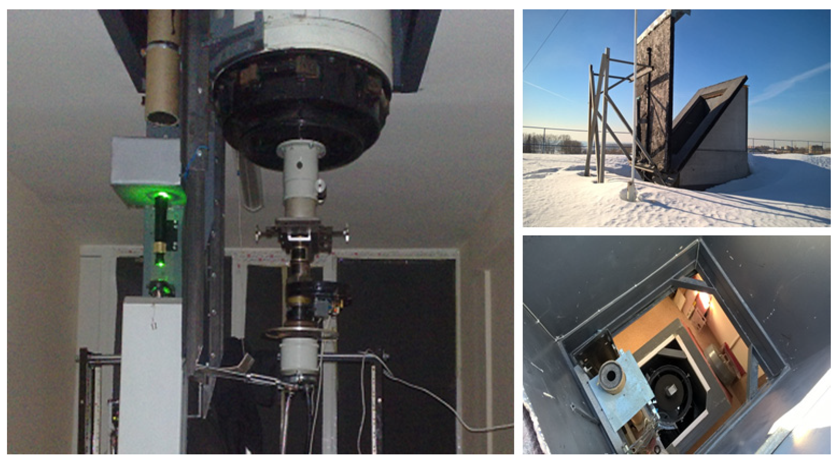
2.1. High-Altitude Matrix Polarization Lidar (HAMPL)
2.2. Meteorological Conditions at the Altitudes of Clouds Registered by the Lidar
2.3. Machine Learning Techniques
- (1)
- Determine the probability of observation of HLCs depending on meteorological parameters (classification task);
- (2)
- Make a preliminary estimation of the observation altitude and boundaries of HLCs depending on meteorological parameters (regression task);
- (3)
- Estimate BSPM values using meteorological parameters (regression task).
3. Results
- -
- Dimensionality reduction in the ERA5 reanalysis data;
- -
- Analysis of the relationship between the altitude of HLC detection and meteorological parameters;
- -
- Determination of BSPM based on meteorological parameters.
3.1. Preliminary Analysis
3.2. Implementation of Data Dimensionality Reduction
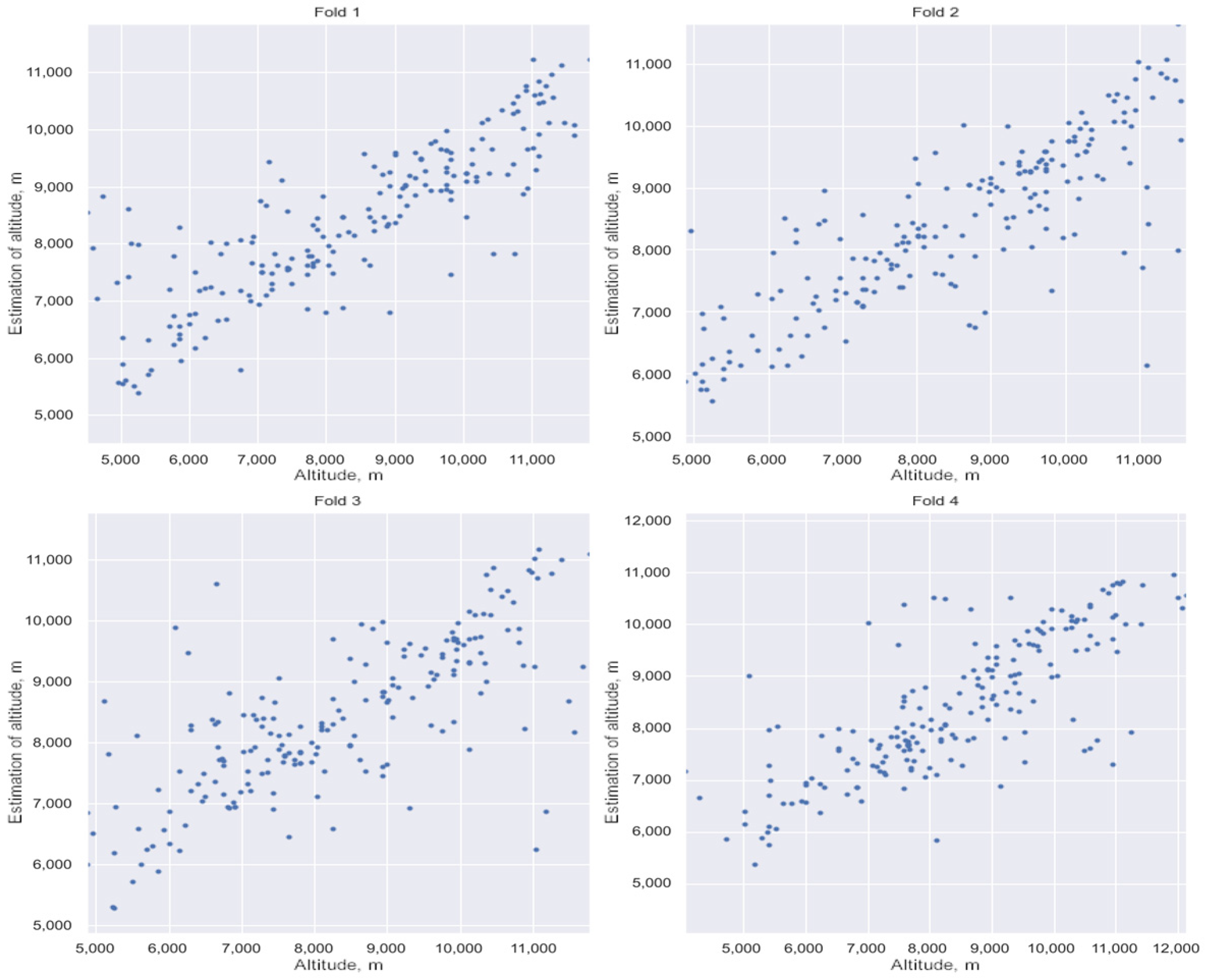
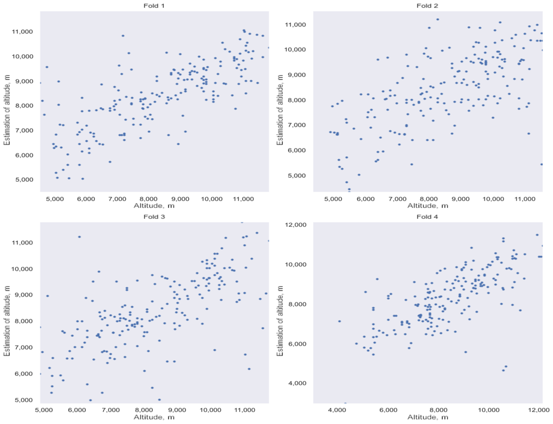
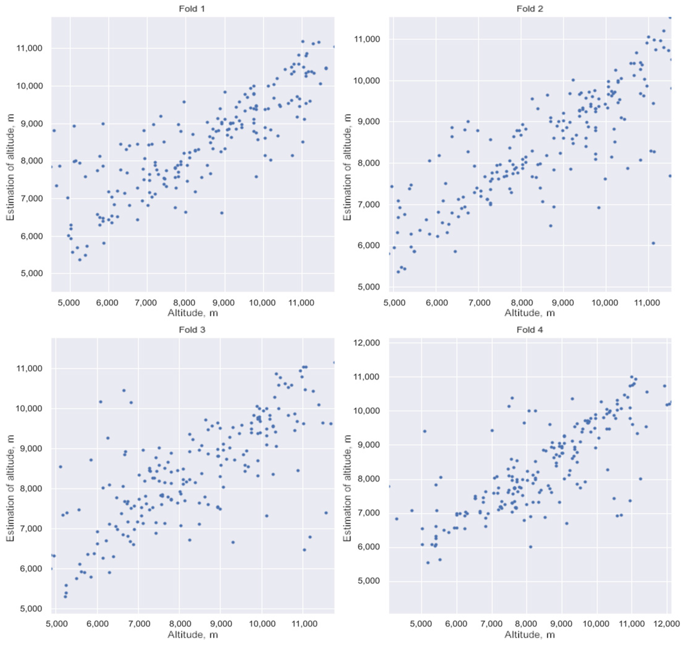
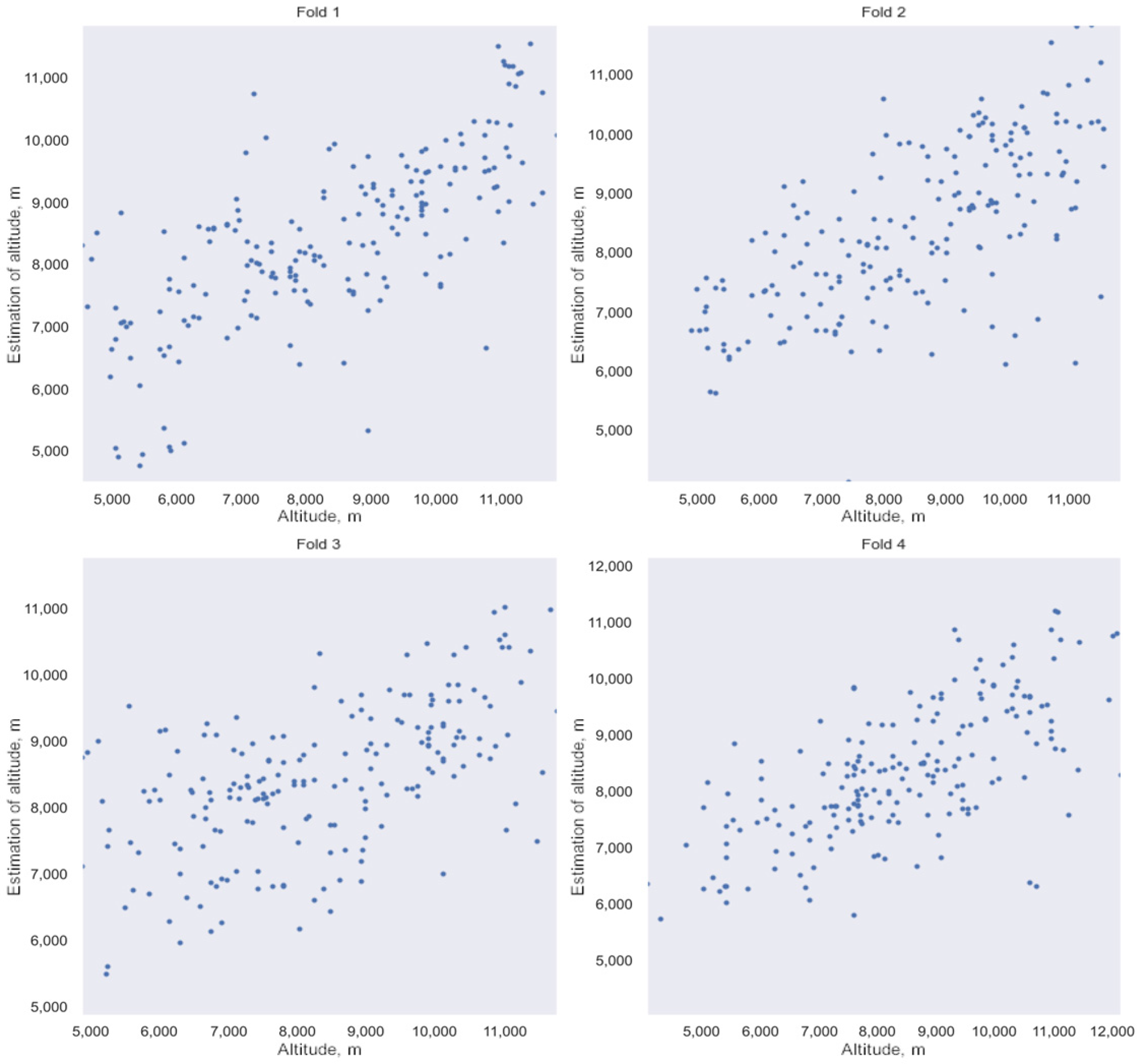
3.3. Estimation of HLC Detection Altitude
- The current part forms the test sample;
- The remaining parts form the training sample;
- Training of the neural network on the training sample and calculation of the standard deviation on the test sample.
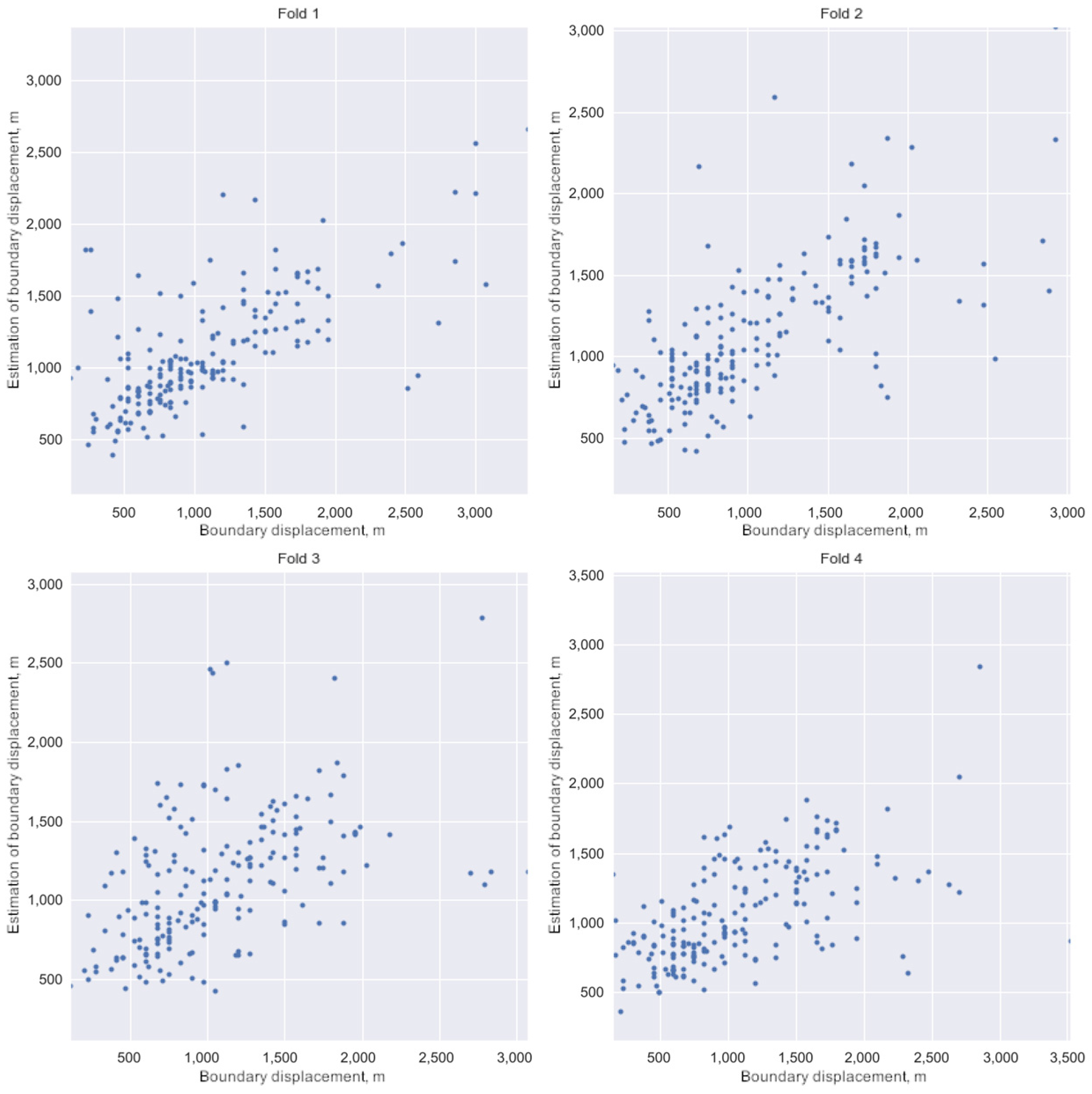
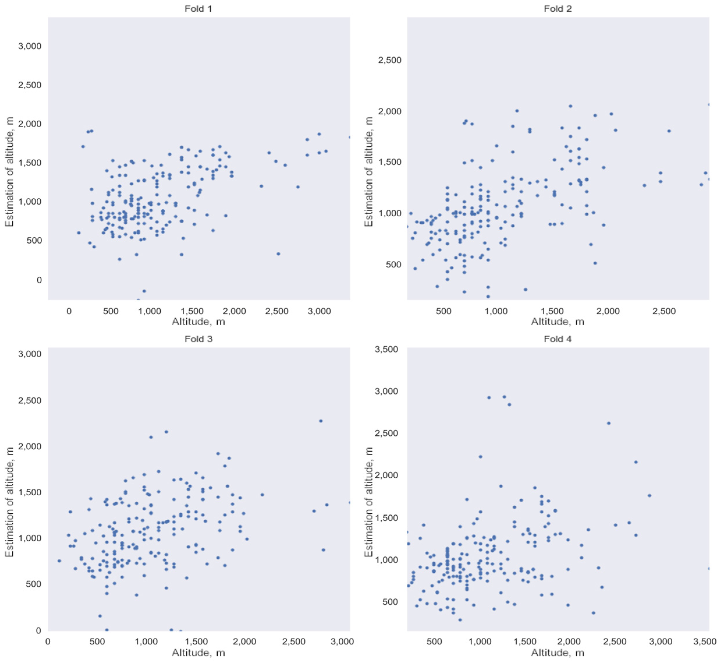
3.4. Defining HLC Boundaries
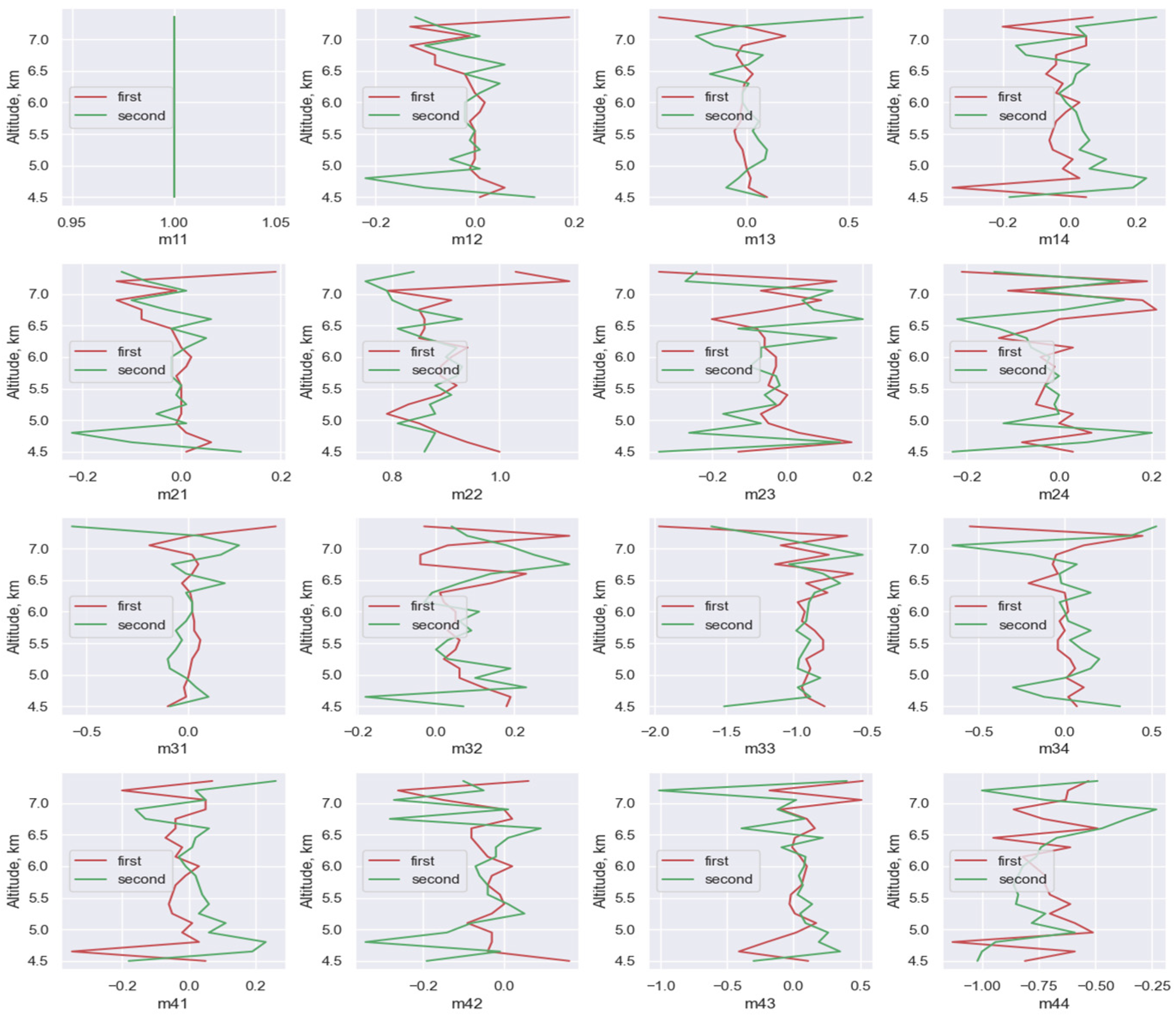
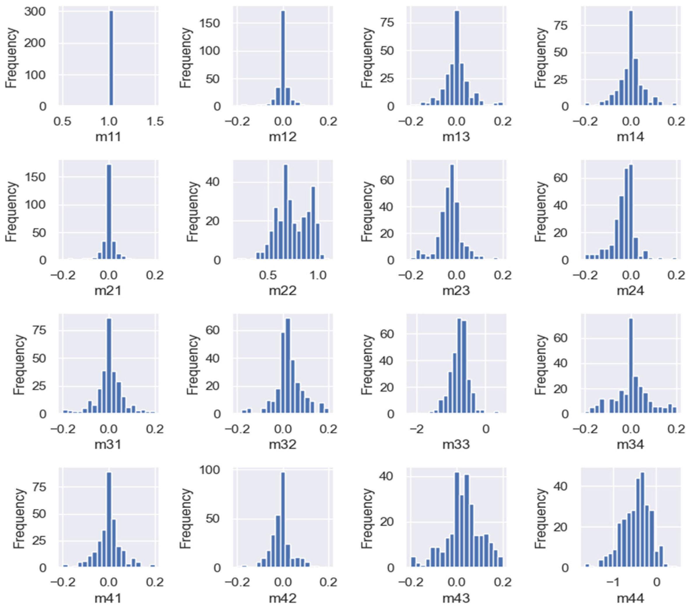
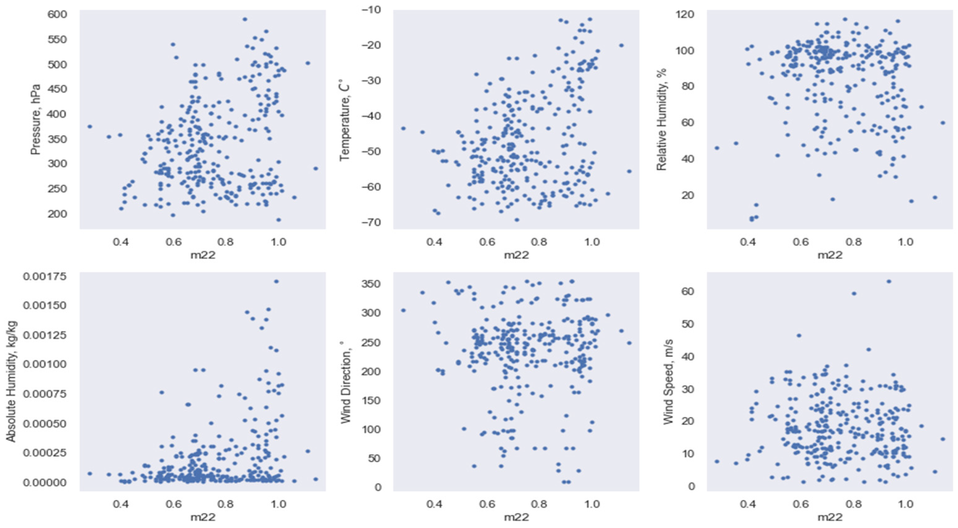
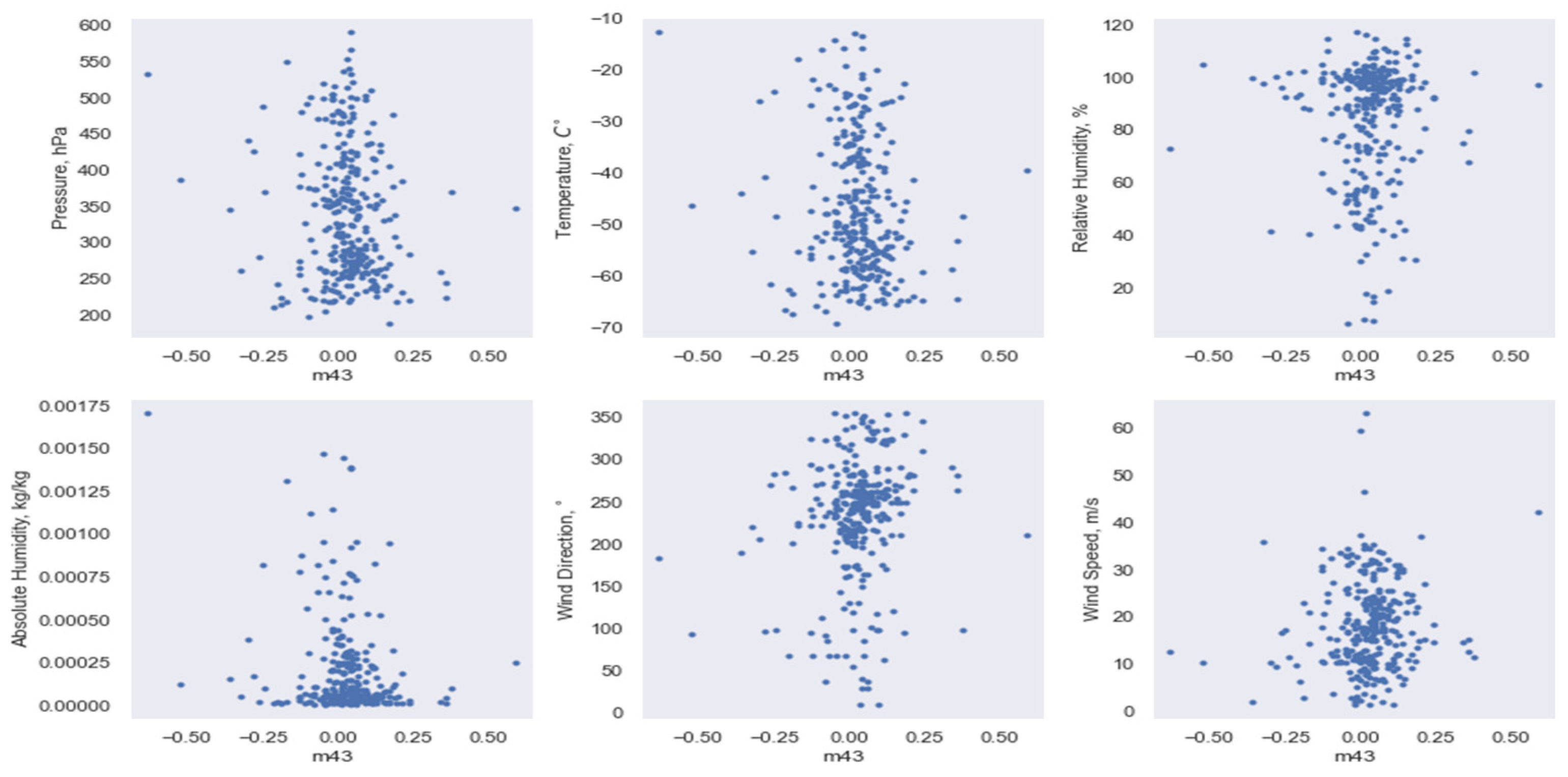
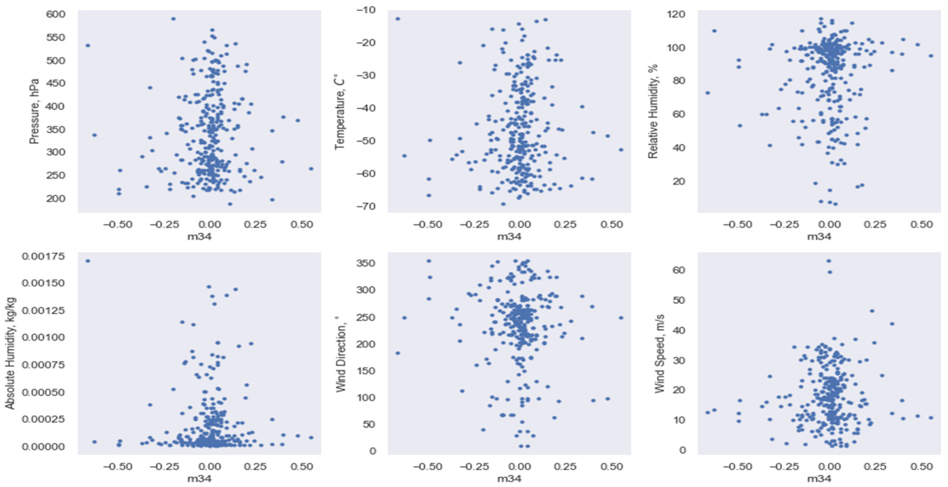
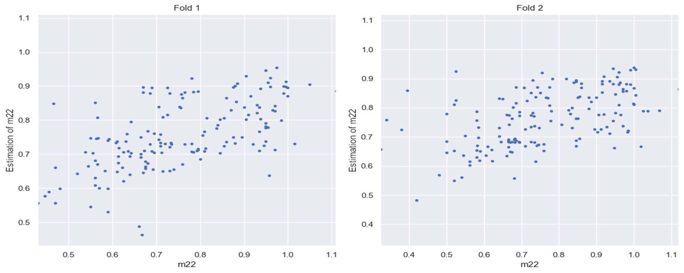
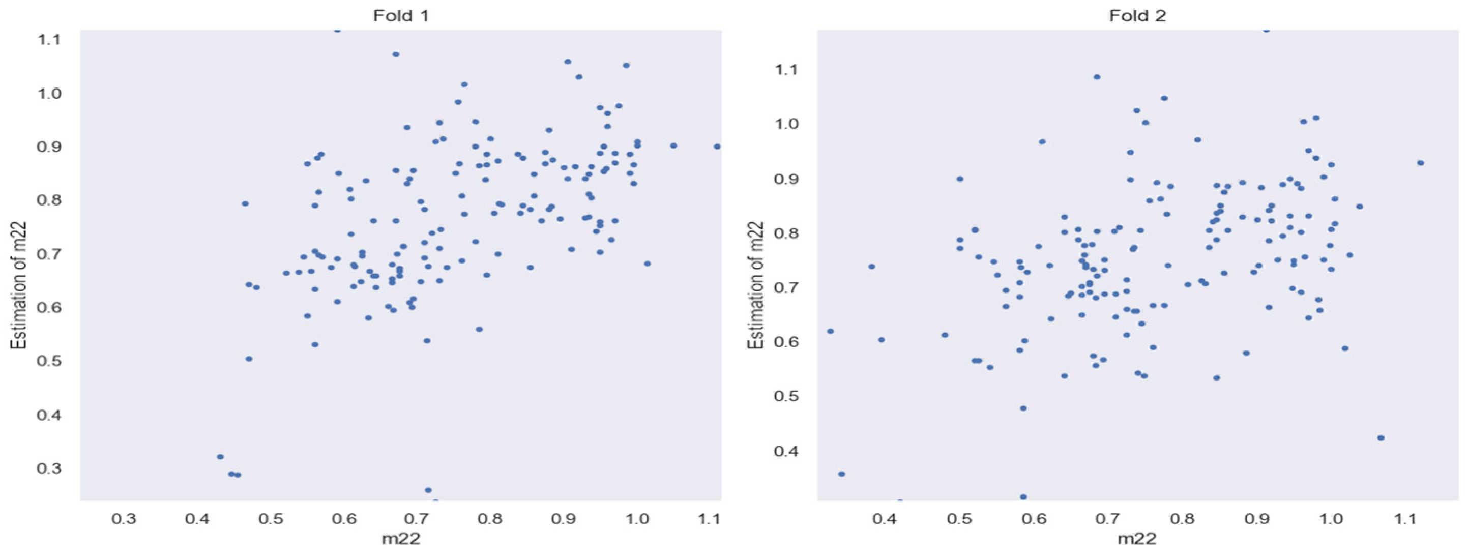
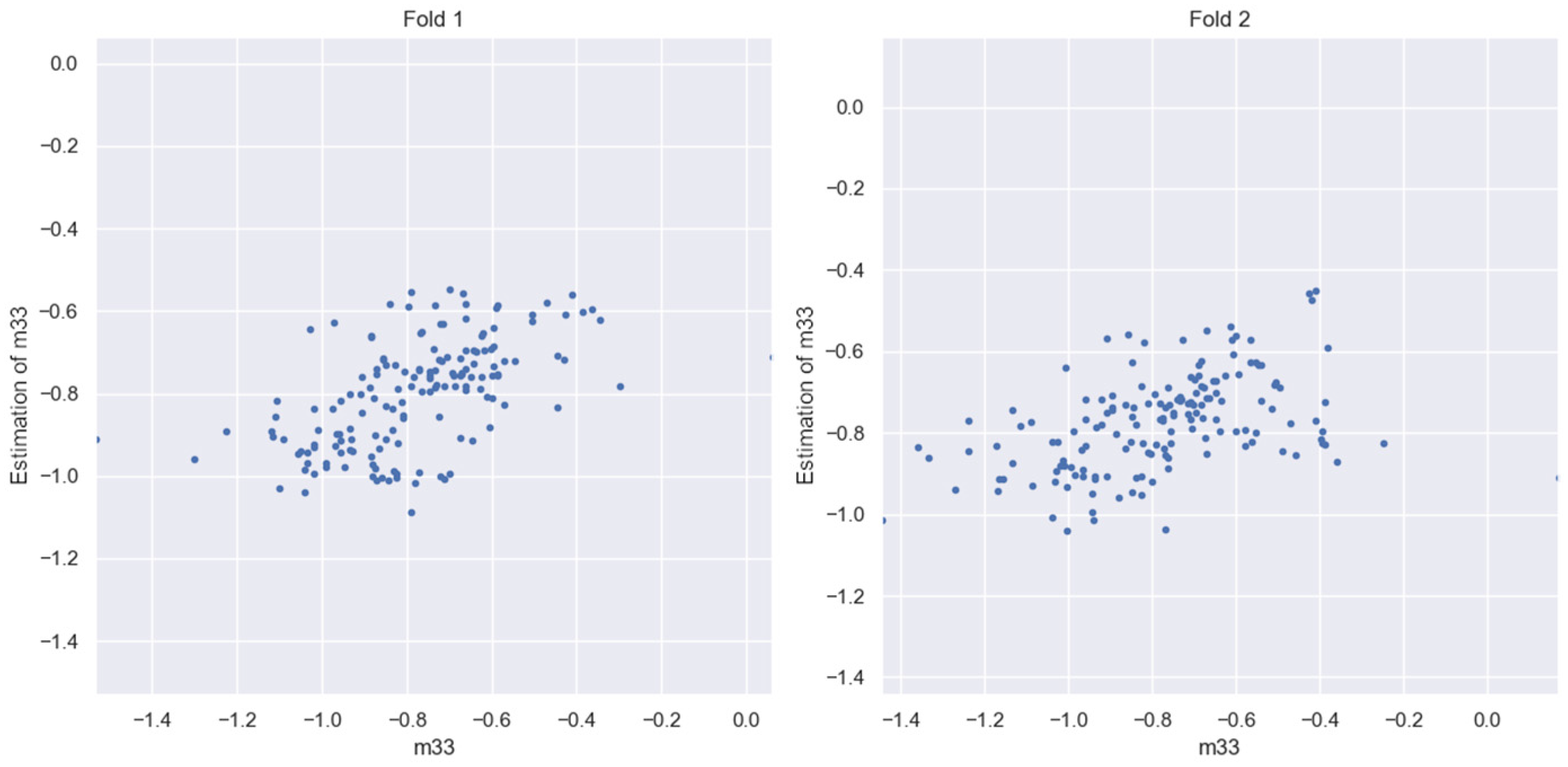
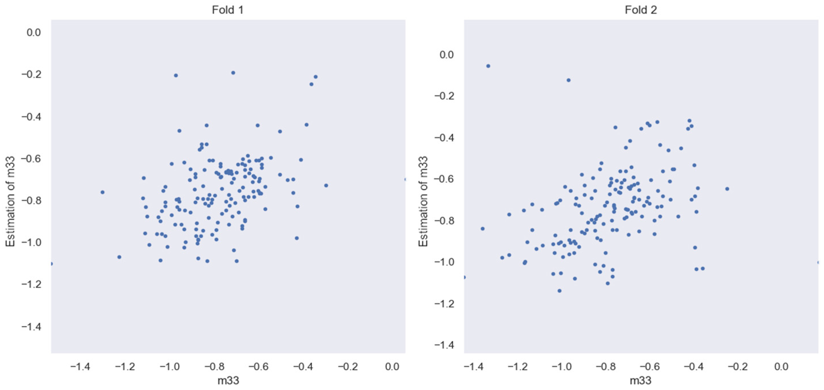
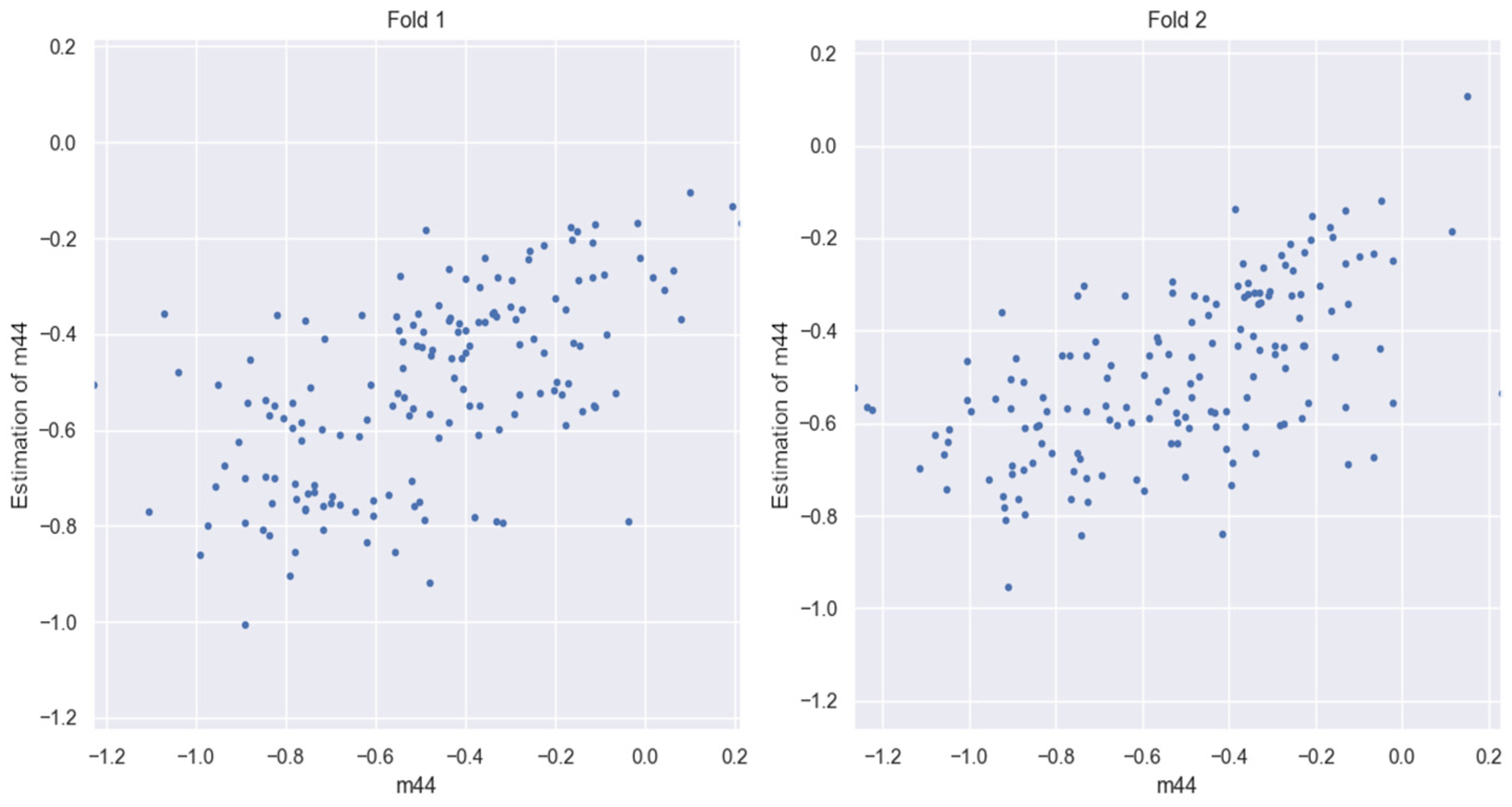
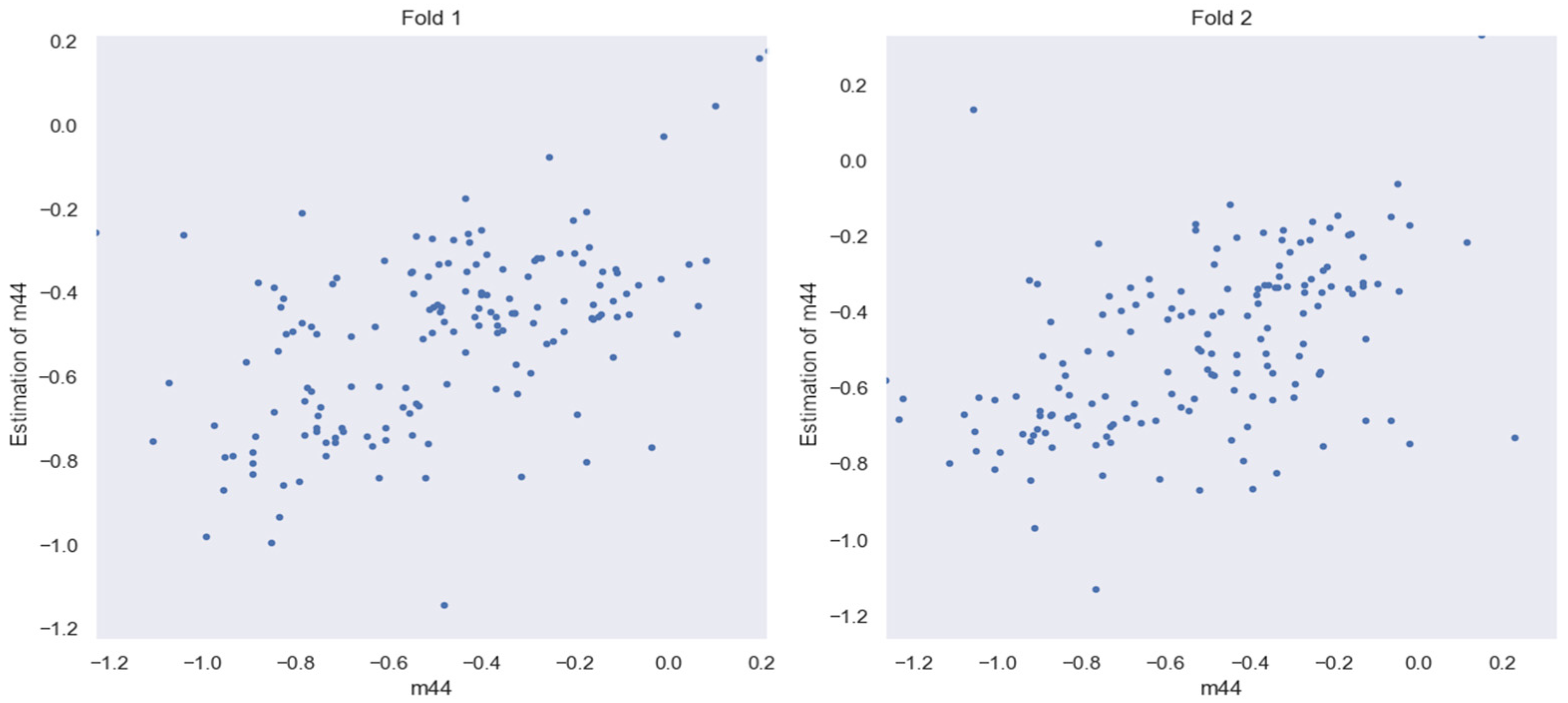
3.5. Evaluation of HLC BSPM Elements
4. Discussion
5. Conclusions
Author Contributions
Funding
Institutional Review Board Statement
Informed Consent Statement
Data Availability Statement
Conflicts of Interest
References
- Yeganeh-Bakhtiary, A.; EyvazOghli, H.; Shabakhty, N.; Kamranzad, B.; Abolfathi, S. Machine learning as a downscaling approach for prediction of wind characteristics under future climate change scenarios. Complexity 2022, 2022, 8451812. [Google Scholar]
- Donnelly, J.; Abolfathi, S.; Pearson, J.; Chatrabgoun, O.; Daneshkhah, A. Gaussian process emulation of spatio-temporal outputs of a 2D inland flood model. Water Res. 2022, 225, 119100. [Google Scholar] [CrossRef] [PubMed]
- Nourani, V.; Khodkar, K.; Paknezhad, N.J.; Laux, P. Deep learning-based uncertainty quantification of groundwater level predictions. Stoch. Environ. Res. Risk Assess 2022, 36, 3081–3107. [Google Scholar] [CrossRef]
- Zennaro, F.; Furlan, E.; Simeoni, C.; Torresan, S.; Aslan, S.; Critto, A.; Marcomini, A. Exploring machine learning potential for climate change risk assessment. Earth-Sci. Rev. 2021, 220, 103752. [Google Scholar] [CrossRef]
- Sattari, M.T.; Mirabbasi, R.; Sushab, R.S.; Abraham, J. Prediction of groundwater level in Ardebil plain using support vector regression and M5 tree model. Groundwater 2018, 56, 636–646. [Google Scholar] [CrossRef] [PubMed]
- Kim, I.; Kim, B.; Sidorov, D. Machine Learning for Energy Systems Optimization. Energies 2022, 15, 4116. [Google Scholar] [CrossRef]
- Feigelson, E.M. (Ed.) Radiation Properties of Perispheric Clouds; Nauka: Moscow, Russia, 1989. (In Russian) [Google Scholar]
- Winker, D.M.; Trepte, C.R. Laminar cirrus observed near the tropical tropopause by LITE. Geophys. Res. Lett. 1998, 25, 3351–3354. [Google Scholar] [CrossRef]
- Liou, K.N. Influence of cirrus clouds on weather and climate processes: A global perspective. J. Geophys. Res. 1986, 103, 1799–1805. [Google Scholar] [CrossRef]
- Sassen, K.; Griffin, M.K.; Dodd, G.C. Optical scattering, and microphysical properties of subvisual cirrus clouds, and climatic implications. J. Appl. Meteorol. 1989, 28, 91–98. [Google Scholar] [CrossRef]
- Dmitrieva-Arrago, L.R.; Trubina, M.A.; Tolstyh, M.A. Role of Phase Composition of Clouds in Forming High and Low Frequency Radiaion. Proc. Hydrometeorol. Res. Cent. Russ. Fed. 2017, 363, 19–34. (In Russian) [Google Scholar]
- Stengel, M.; Meirink, J.F.; Eliasson, S. On the Temperature Dependence of the Cloud Ice Particle Effective Radius—A Satellite Perspective. Geophys. Res. Lett. 2023, 50, e2022GL102521. [Google Scholar] [CrossRef]
- Scientific and Technological Infrastructure of the Russian Federation. Radiophysical Complex: High-Altitude Polarization Lidar for Atmospheric Sensing and Tomsk Ionospheric Station “LIDAR-IONOSONDE”. Available online: https://ckp-rf.ru/catalog/usu/73573 (accessed on 25 November 2023).
- Guasta, M.D.; Vallar, E.; Riviere, O.; Castagnoli, F.; Venturi, V.; Morandi, M. Use of polarimetric lidar for the study of oriented ice plates in clouds. Appl. Opt. 2006, 45, 4878–4887. [Google Scholar] [CrossRef] [PubMed]
- Hayman, M.; Thayer, J.P. General description of polarization in lidar using Stokes vectors and polar decomposition of Mueller matrices. J. Opt. Soc. Am. 2012, 29, 400–409. [Google Scholar] [CrossRef] [PubMed]
- Volkov, S.N.; Samokhvalov, I.V.; Cheong, D.H.; Kim, D. Investigation of East Asian clouds with polarization light detection and ranging. Appl. Opt. 2015, 54, 3095–3105. [Google Scholar] [CrossRef]
- Kokhanenko, G.P.; Balin, Y.S.; Klemasheva, M.G.; Nasonov, S.V.; Novoselov, M.M.; Penner, I.E.; Samoilova, S.V. Scanning polarization lidar LOSA-M3: Opportunity for research of crystalline particle orientation in the ice clouds. Atmos. Meas. Tech. 2020, 13, 1113–1127. [Google Scholar] [CrossRef]
- Kuchinskaia, O.; Bryukhanov, I.; Penzin, M.; Ni, E.; Doroshkevich, A.; Kostyukhin, V.; Samokhvalov, I.; Pustovalov, K.; Bordulev, I.; Bryukhanova, V.; et al. ERA5 Reanalysis for the Data Interpretation on Polarization Laser Sensing of High-Level Clouds. Remote Sens. 2023, 15, 109. [Google Scholar] [CrossRef]
- Central Aerological Observatory. Available online: http://cao-ntcr.mipt.ru/monitor/locator.htm (accessed on 1 February 2024).
- University of Wyoming. Available online: http://weather.uwyo.edu (accessed on 1 February 2024).
- Penzin, M.S.; Bryukhanov, I.D.; Kuchinskaia, O.I.; Ni, E.V.; Pustovalov, K.N.; Zhivotenyuk, I.V.; Doroshkevich, A.A.; Bordulev Iu, S.; Samohvalov, I.V. Verification of ERA5 reanalysis data for the interpretation of lidar investigation of high-level clouds. In Proceedings of the SPIE 28th International Symposium on Atmospheric and Ocean Optics: Atmospheric Physics, Tomsk, Russia, 4–8 July 2022; Volume 12341, p. 4. [Google Scholar] [CrossRef]
- Copernicus Climate Data Store. Available online: https://cds.climate.copernicus.eu (accessed on 1 February 2024).
- Kaul, B.V.; Samokhvalov, I.V.; Volkov, S.N. Investigating particle orientation in cirrus clouds by measuring backscattering phase matrices with lidar. Appl. Opt. 2004, 43, 6620–6628. [Google Scholar] [CrossRef]


| Temperature (°C) | Relative Humidity (kg*kg−1) | Absolute Humidity (%) | Wind Speed (m/s2) | |
|---|---|---|---|---|
| PCA | 2.36 | 60.7 | 0.57 × 0−7 | 1.61 |
| AE | 1.66 | 42.54 | 0.51 × 10⁻⁷ | 1.58 |
| RF (PCA) | NN (PCA) | RF (AE) | NN (AE) | |
|---|---|---|---|---|
| Fold 1 | 1097.07 | 1232.56 | 1162.26 | 1320.61 |
| Fold 2 | 1048.35 | 1350.06 | 1065.12 | 1371.62 |
| Fold 3 | 1177.63 | 1433.94 | 1181.13 | 1383.15 |
| Fold 4 | 1095.24 | 1222.92 | 1150.78 | 1388.10 |
| RF (PCA) | NN (PCA) | RF (AE) | NN (AE) | |
|---|---|---|---|---|
| Fold 1 | 458.60 | 557.44 | 458.91 | 548.99 |
| Fold 2 | 420.30 | 494.86 | 454.43 | 510.57 |
| Fold 3 | 491.13 | 520.78 | 498.08 | 582.19 |
| Fold 4 | 488.48 | 603.55 | 488.23 | 549.19 |
| RF (PCA) | NN (PCA) | RF (AE) | NN (AE) | |
|---|---|---|---|---|
| Fold 1 | 0.12 | 0.14 | 0.12 | 0.17 |
| Fold 2 | 0.14 | 0.16 | 0.13 | 0.19 |
| RF (PCA) | NN (PCA) | RF (AE) | NN (AE) | |
|---|---|---|---|---|
| Fold 1 | 0.17 | 0.20 | 0.18 | 0.21 |
| Fold 2 | 0.21 | 0.25 | 0.22 | 0.22 |
| RF (PCA) | NN (PCA) | RF (AE) | NN(AE) | |
|---|---|---|---|---|
| Fold 1 | 0.24 | 0.25 | 0.18 | 0.20 |
| Fold 2 | 0.25 | 0.28 | 0.21 | 0.22 |
Disclaimer/Publisher’s Note: The statements, opinions and data contained in all publications are solely those of the individual author(s) and contributor(s) and not of MDPI and/or the editor(s). MDPI and/or the editor(s) disclaim responsibility for any injury to people or property resulting from any ideas, methods, instructions or products referred to in the content. |
© 2024 by the authors. Licensee MDPI, Basel, Switzerland. This article is an open access article distributed under the terms and conditions of the Creative Commons Attribution (CC BY) license (https://creativecommons.org/licenses/by/4.0/).
Share and Cite
Kuchinskaia, O.; Penzin, M.; Bordulev, I.; Kostyukhin, V.; Bryukhanov, I.; Ni, E.; Doroshkevich, A.; Zhivotenyuk, I.; Volkov, S.; Samokhvalov, I. Artificial Neural Networks for Determining the Empirical Relationship between Meteorological Parameters and High-Level Cloud Characteristics. Appl. Sci. 2024, 14, 1782. https://doi.org/10.3390/app14051782
Kuchinskaia O, Penzin M, Bordulev I, Kostyukhin V, Bryukhanov I, Ni E, Doroshkevich A, Zhivotenyuk I, Volkov S, Samokhvalov I. Artificial Neural Networks for Determining the Empirical Relationship between Meteorological Parameters and High-Level Cloud Characteristics. Applied Sciences. 2024; 14(5):1782. https://doi.org/10.3390/app14051782
Chicago/Turabian StyleKuchinskaia, Olesia, Maxim Penzin, Iurii Bordulev, Vadim Kostyukhin, Ilia Bryukhanov, Evgeny Ni, Anton Doroshkevich, Ivan Zhivotenyuk, Sergei Volkov, and Ignatii Samokhvalov. 2024. "Artificial Neural Networks for Determining the Empirical Relationship between Meteorological Parameters and High-Level Cloud Characteristics" Applied Sciences 14, no. 5: 1782. https://doi.org/10.3390/app14051782
APA StyleKuchinskaia, O., Penzin, M., Bordulev, I., Kostyukhin, V., Bryukhanov, I., Ni, E., Doroshkevich, A., Zhivotenyuk, I., Volkov, S., & Samokhvalov, I. (2024). Artificial Neural Networks for Determining the Empirical Relationship between Meteorological Parameters and High-Level Cloud Characteristics. Applied Sciences, 14(5), 1782. https://doi.org/10.3390/app14051782