1. Introduction
The AERORail Transportation System is a new type of transportation system in the form of a cable-supported rail combined structure composed of multi-span continuous string cables, rails, lower supports and related power supply and control systems [
1]. The load bearing system of AERORail consists of two rails supported by prestressed cables. AERORail is advantageous for its reduced construction cost and time, which are attributed to its simplified structure and lightweight design. A full-scale model of AERORail was reported by Li et al. [
2], who studied the full-scale model’s acceleration and displacement response under a two-axle vehicle. Besides the structural responses during the vibration, the contact force between the vehicle and the structure is also an intriguing topic [
3,
4]. Based on fundamental frequency analysis of the structure and the dynamic load test, the variation of the contact force in AERORail was studied and identified using the time domain identification method by Li et al. [
5] in the previous study. It was proved that the occurrence time and frequency of the contact force are highly related to the passing time of the vehicle. However, the study was based on a limited number of experiments and was limited to low speed and 5–10 m spans. The vibration of large-span AERORail systems under high-speed vehicles is still open to discussion. Besides the absence of this knowledge, there is also a gap between the experiment data and a convincing model that depicts the variation of the contact force, which is essentially a load to the structure. Though a vehicle-structure model for the AERORail was reported by Li et al. [
5], a load model applicable to static or dynamic analyses of AERORail is yet to be found. Due to the difference between the characteristics of the AERORail and conventional structures, it is necessary to investigate the contact force and devise a load model in order to promote the AERORail to its application.
The traditional way to estimate the live load to a bridge is by survey or the weigh-in-motion system [
6,
7]. These methods are designed to obtain the probability density of distribution for multiple vehicle types. As was discussed by Li et al. [
5], the force between the vehicle and structure shows dramatic fluctuation due to the vibration, therefore the axle weight of the vehicle cannot be regarded as the contact force. The weight-in-motion system is also inapplicable for the current study due to the no-deck design of AERORail. Thus, an alternative approach must be utilized to obtain the load model based on the history of the contact force.
This paper used Bezier curves to establish a time-history load model of the AERORail structure by approximating the contact force from Li et al. [
2]. The contact force was identified from the acceleration data of the structure during vehicle running. In order to validate the load model obtained, the displacement response of AERORail under the proposed load curves was compared to available experiment data. Furthermore, the structural response of large spans under high-speed vehicles was investigated via the proposed load model.
2. Data Fitting and Bezier Curves
Data fitting is a commonly used method in research to summarize empirical laws, which can find trend rules from measured data or simulation results simply and effectively [
8,
9]. For data that are discrete and random, the commonly used fitting methods include least squares, maximum likelihood estimation, etc. The least squares method refers to determining the best fit for the original data
by choosing a function
that minimizes the sum of the squares of the differences for a given set of data [
10]. This process can be represented by Equation (1):
where
is the error function, and
N is the total number of sample points. Generally speaking, directly obtaining the expression of the fitting function is difficult. Usually, a fitting function (Equation (2)) is determined using a set of basis functions and variable parameters:
where
and
are the basis functions and the variable parameters, respectively. Once the basis functions are selected, the actual problem becomes solving for
. With
, the expression of the fitting function can be obtained through Equation (2). There are various choices for the basis functions of the fitting function, including polynomial, sine function, power function, and exponential function, etc. For the contact force’s time-history curve to be analyzed, due to its relatively uniform curve shape (double-valley curve or single-valley curve), traditional polynomial fitting is feasible [
11,
12]. However, in polynomial fitting, the physical meanings of the coefficients are not very clear, and most of the time researchers cannot derive further rules or gain any intuitive understanding of it, which hinders further in-depth research. In addition, considering that the contact force’s time-history curve contains many high-frequency low-amplitude vibrations, and these have little impact on the structure because the vibrational response of the structure is mainly caused by low-frequency vibrations within its fundamental frequency range, the chosen basis function for fitting should ideally disregard this part of the vibration.
Besides polynomial and other basis functions, there are Bezier curves [
13,
14], B-spline curves [
15,
16], and non-uniform rational B-splines (NURBS) [
17] available in the field of data analysis. Among these, Bezier curves have the advantages of simple form, smooth curvature, easy calculation, and easy implementation, and have been widely used in fields such as CAD, artistic design, and complex shape modeling. Bezier curves determine the shape and position of the curve through a finite number of control points, and the visually smooth curves determined by the control points are also an important method for vector graphics. Using Bezier curves as the basis function for fitting the contact force time-history curve can effectively address the issues mentioned earlier, and Bezier curves themselves have good parameterization capabilities, making it convenient for future research to start from the curve control points and explore deeper patterns [
18,
19].
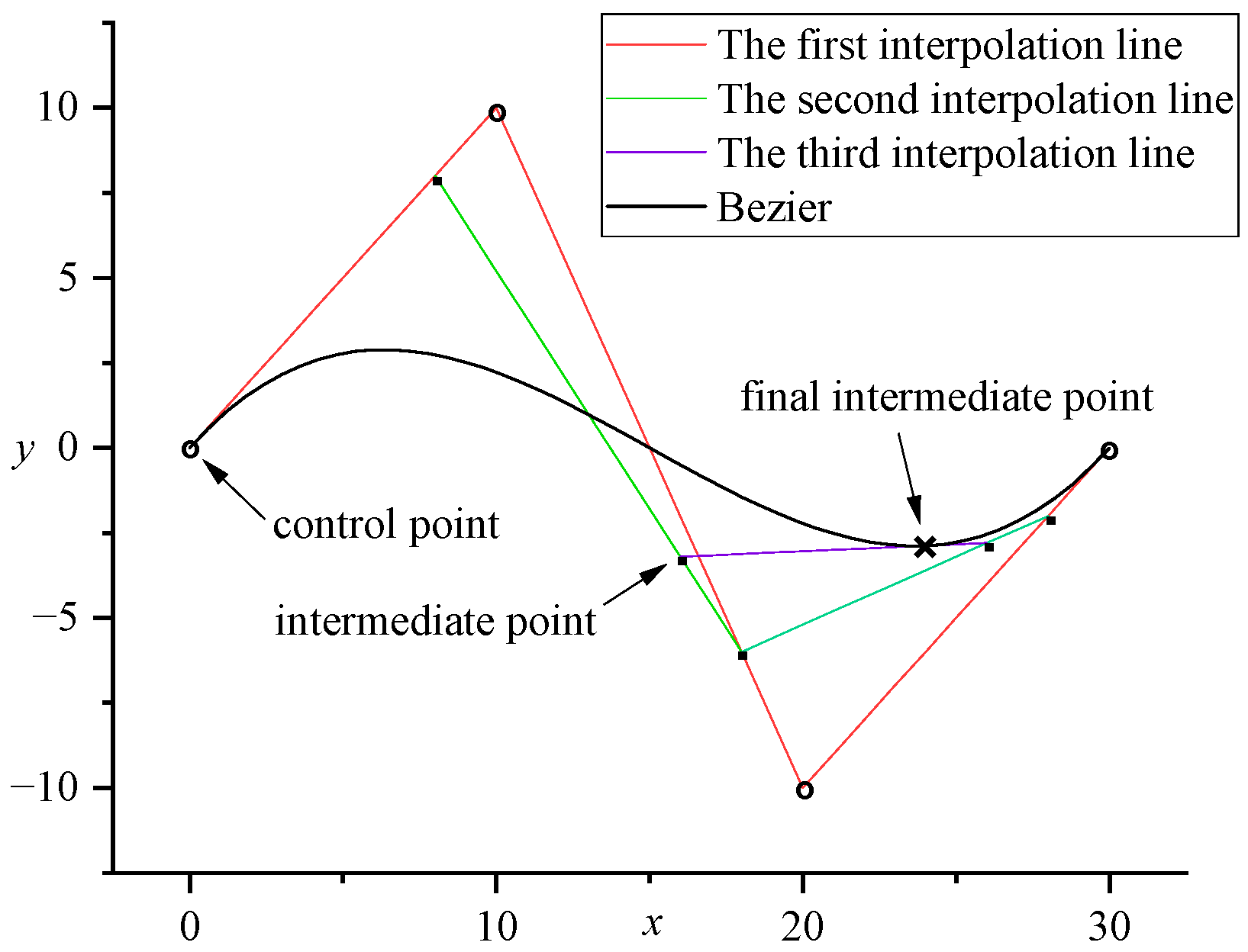
A Bezier curve is obtained by recursively inserting points to interpolation lines connecting consecutive control points and inserted points. For
n + 1 control points, one connects these points and inserts
n intermediate points at a local coordinate
t on each interpolation line. These intermediate points are then treated as the new control points and the above step is repeated to get new intermediate points. After the recursion, there is only one intermediate point left. If the value of
t is changed (e.g., from 0.5 to 0.75), the final intermediate point will also move accordingly, thereby generating a smooth trajectory in space. This trajectory is the Bezier curve. The expression of the Bezier curve can be determined by the parameter
t and the coordinates of
n + 1 control points (Equation (3)):
where
is the expression of the Bezier curve,
are the coordinates of the control points,
t is the independent variable parameter of the curve, and
is the Bernstein basis function of degree
n (Equation (4)):
If the above equation is rewritten in matrix form, it can be expressed as (Equation (5)):
Substituting Equation (5) into Equation (3), we obtain Equation (6):
Taking four control points as (0, 0), (10, 10), (20, −10), and (30, 0), the Bezier curve can be drawn as shown in
Figure 1.
Substituting the expression of the Bezier curve from Equation (6) into Equations (1) and (2), we can obtain the least squares fitting Equation (7) based on the Bezier curve basis function:
Using Equation (7) to fit the contact force curve of the AERORail structure from Li et al. [
2], different time-history force models can be obtained.
3. Time-History Contact Force Model
After analyzing the measured data from Li et al. [
2], the authors obtained the time-history curves of contact forces on the elevated track under various conditions and conducted a preliminary exploration. However, if it is to be used for future elevated track design or dynamic research, the current analysis is still insufficient; more general and universally applicable results are needed. This paper establishes an ideal load model, the elevated track time-history force model, which meets the needs of elevated track design and research. It is used for calculating the deflection in different spans of an elevated track in practical applications, serving as a simplified static and dynamic calculation load for practical engineering [
8,
20,
21]. The establishment of the time-history force model will be based on the fitting of the contact force time curves identified by the authors in Li et al. [
2] from the measured data of the elevated track experimental line; for different types of contact force time curves, corresponding time-history force models will be established.
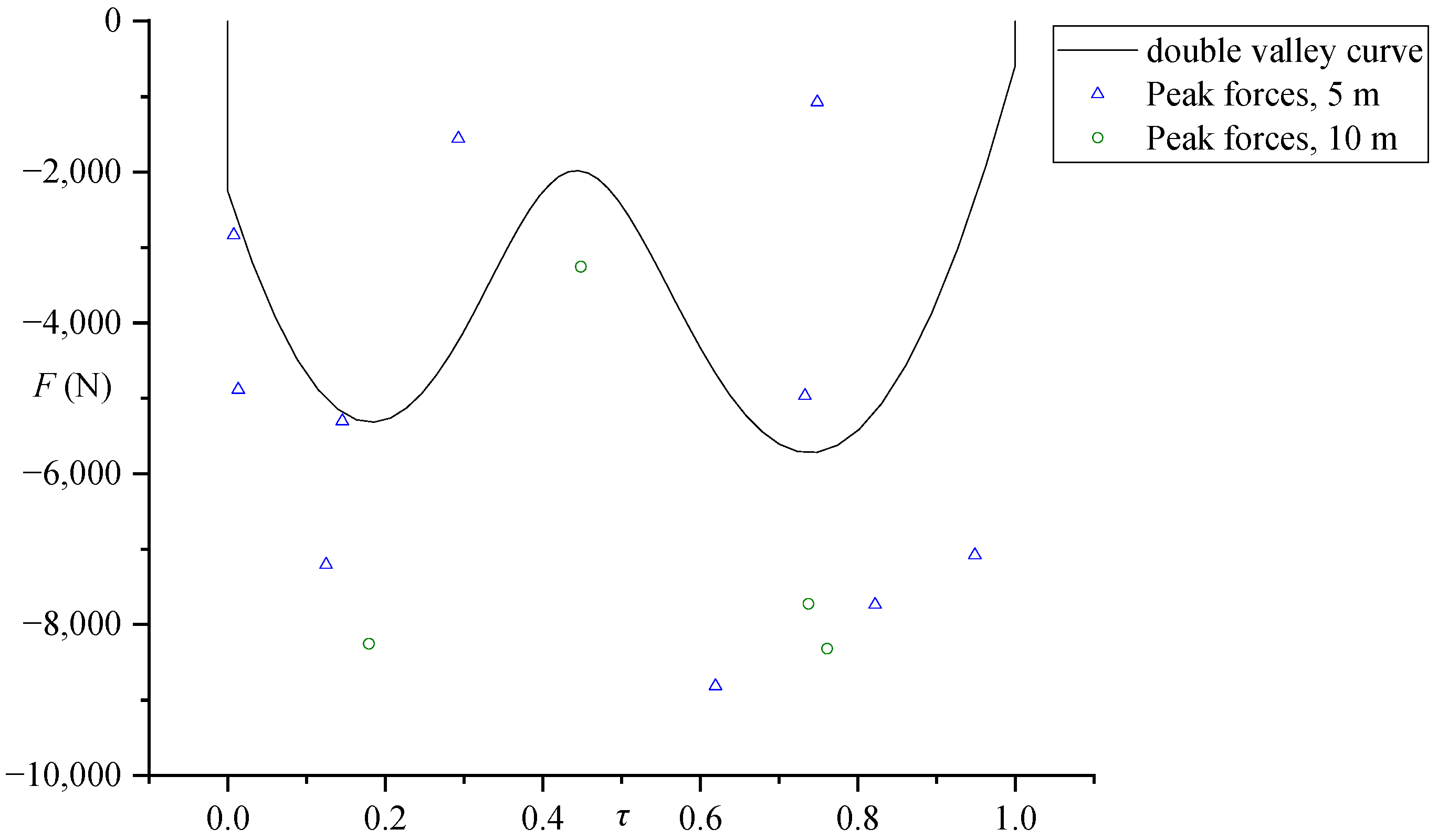
3.1. Standard Double-Valley Curve Model
At a low-speed over the 5 m and 10 m spans, the time-history curves of the contact forces show two valleys, one following the other. This curve shape shows that during the vehicle’s passage over the bridge, there are two impacts on the bridge, and this type of curve shape is referred to as a double-valley curve. In order to obtain a representative standard double-valley curve, this section uses the method of Bezier curve least squares described earlier to fit all double-valley curve sample data.
Although the double-valley curves are similar in shape, their duration varies with the speed of travel (as the speed decreases, the curve duration increases). The analysis results in Li et al. [
2] show that there is no correlation or only a weak correlation between the statistical characteristics of the curve and speed, hence the influence of speed on the curve is only reflected in the duration. In order to eliminate the impact of speed in the standard double-valley curve, a unit duration parameter
is used to replace the actual time
(Equation (8)):
Drawing the contact force curves with double-valley shapes from Li et al. [
2] using the unit duration parameter, an intuitive double-valley curve sample graph is obtained (
Figure 2):
Using Equation (7), the standard double-valley curve as shown in
Figure 3 can be obtained after fitting.
The peak forces of the sample curves from
Figure 2 are also given in
Figure 3 for comparison.
The coordinates of the control points obtained by fitting are shown in
Table 1, and the coordinate table of the control points of the standard double-valley curve.
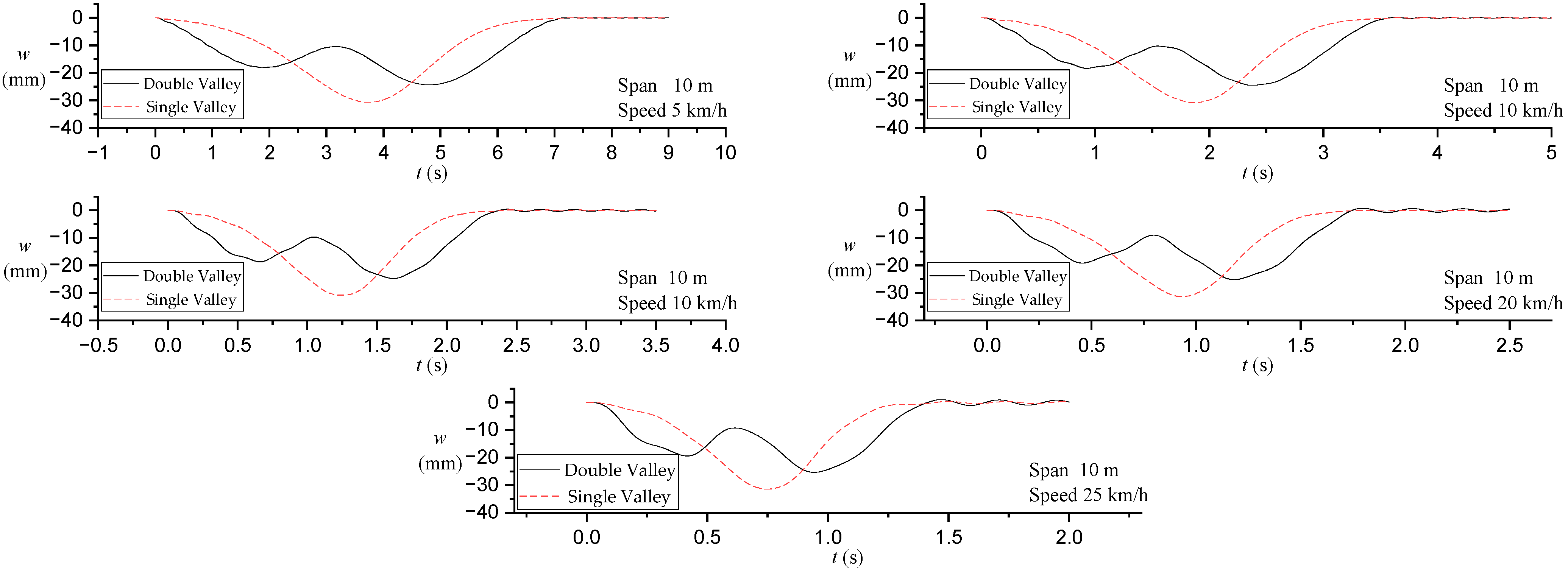
3.2. Standard Double-Valley Curve Working Condition Recalculation
In order to verify whether the established double-valley curve can meet the needs of engineering design under the corresponding working conditions, the simplified dynamics model of AERORail established by Li et al. [
5] and its Simulink simulation system were used for virtual loading. Because the double-valley curve mainly corresponds to the working condition of a 5 m span, only the corresponding working condition was simulated. The working conditions involved in the simulation are shown in
Table 2.
The simulation parameters were calculated using the basic frequency of structure obtained by Li et al. [
5], where the linear density of structure is given as
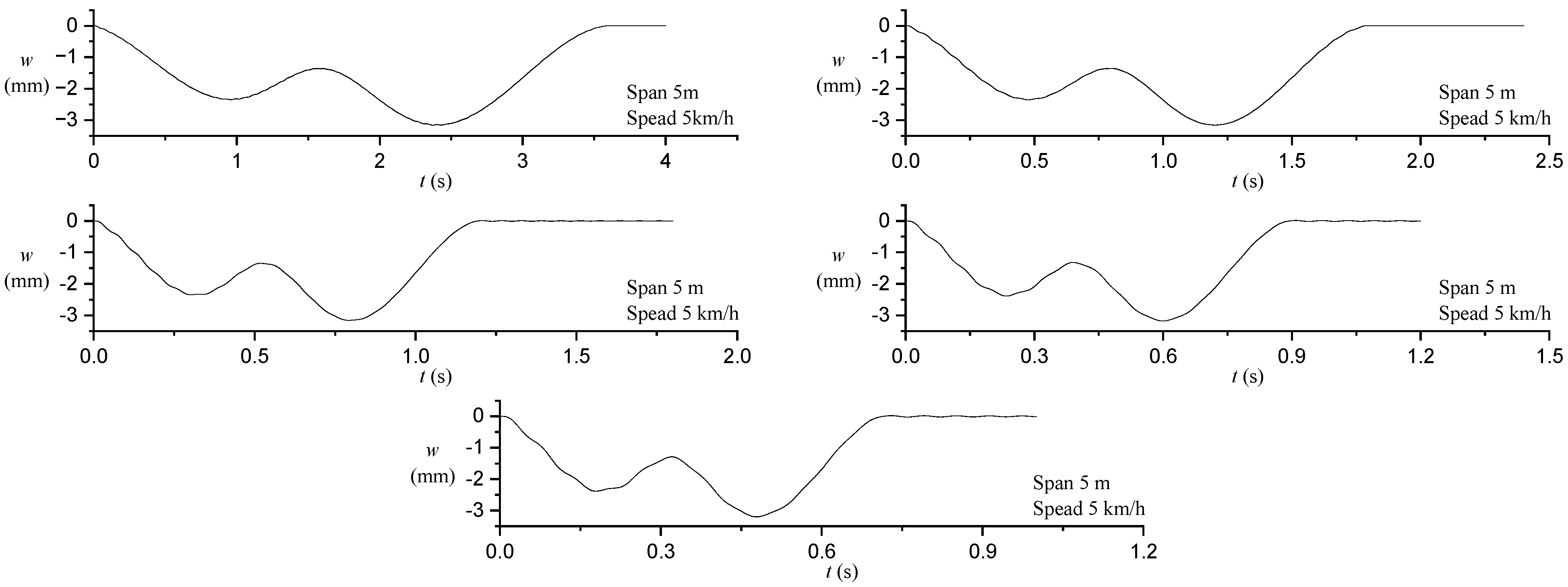
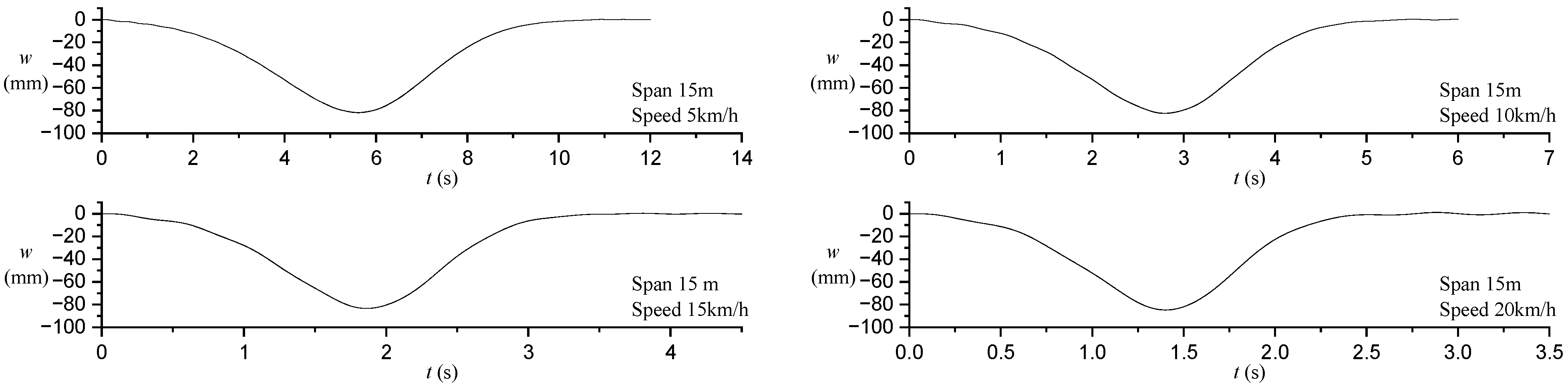
. The cables of 5 m, 10 m, and 15 m spans were all prestressed by 3 tons in advance. After simulation, the mid-span deflection-time diagram under various working conditions was obtained.
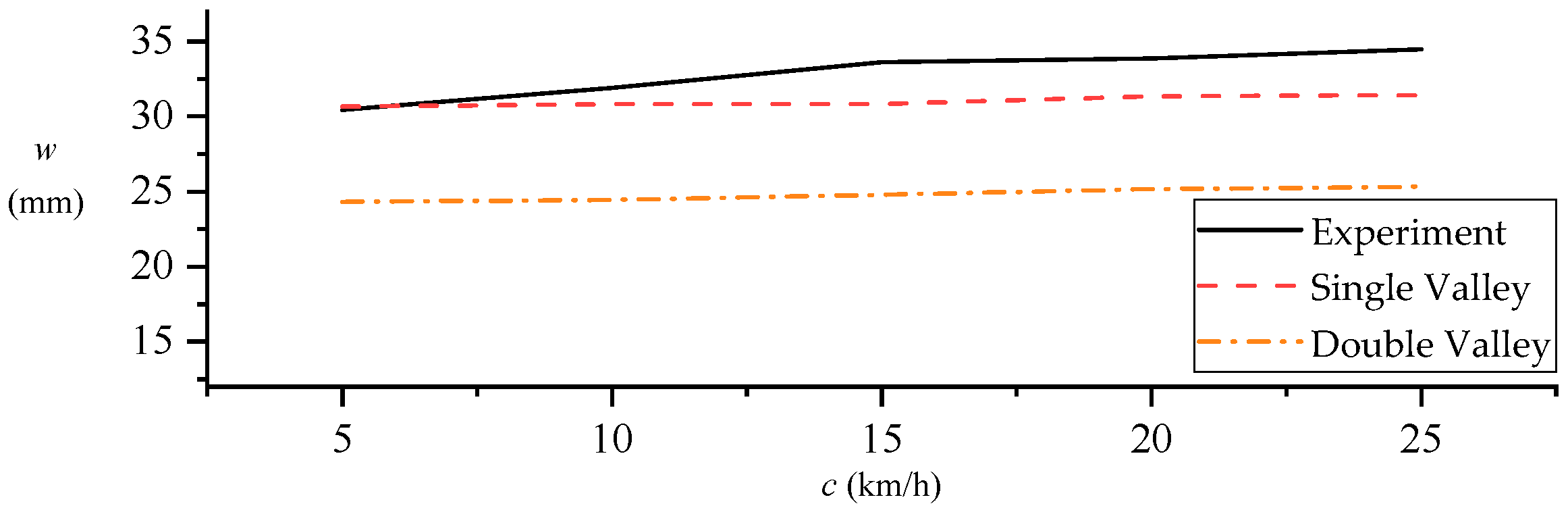
The maximum mid-span deflection of each recalculation condition in
Figure 4 was recorded, and the maximum deflection measured in the experiment was plotted in the figure with the operating speed as the horizontal axis, as shown in
Table 3 and
Figure 5.
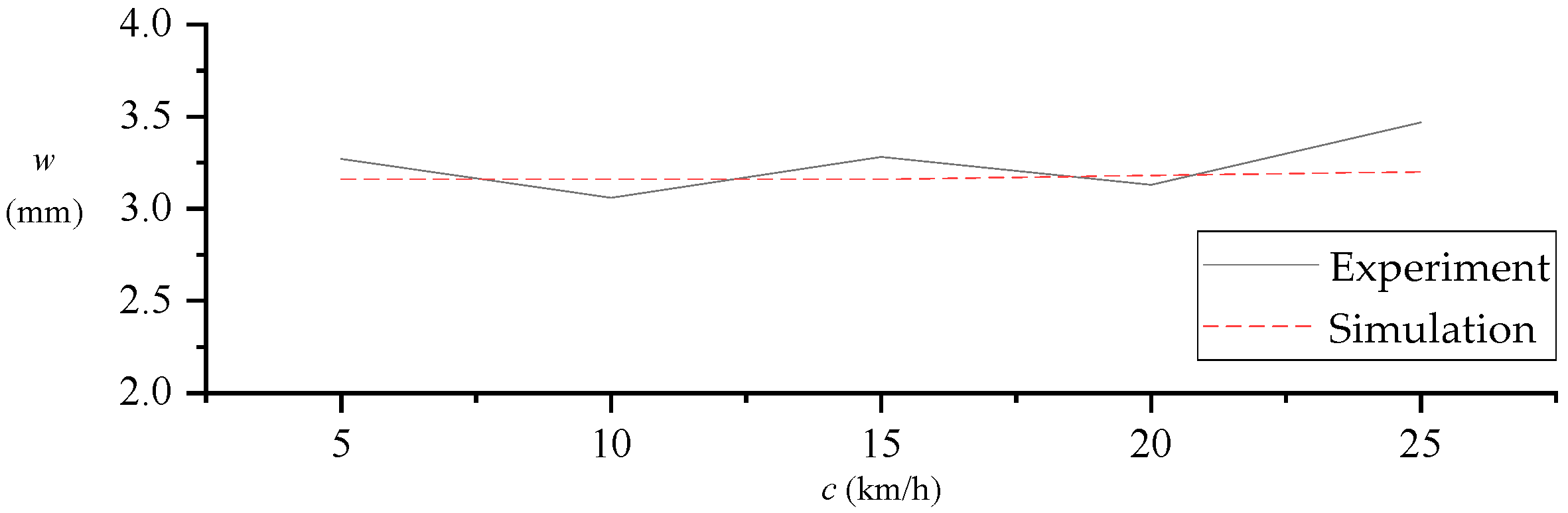
As can be seen from
Table 3 and
Figure 5, the numerical simulation results were relatively close to the actual experimental data at low speed, and the error was less than 4%. Under high-speed conditions, although the relative error was large, it did not increase with the increase of speed. The results show that the standard two-valley curve model has a good reference value for calculating the dynamic response of the AERORail structure with a span of 5 m, and has a good accuracy under low speed conditions, but needs further study under high-speed conditions.
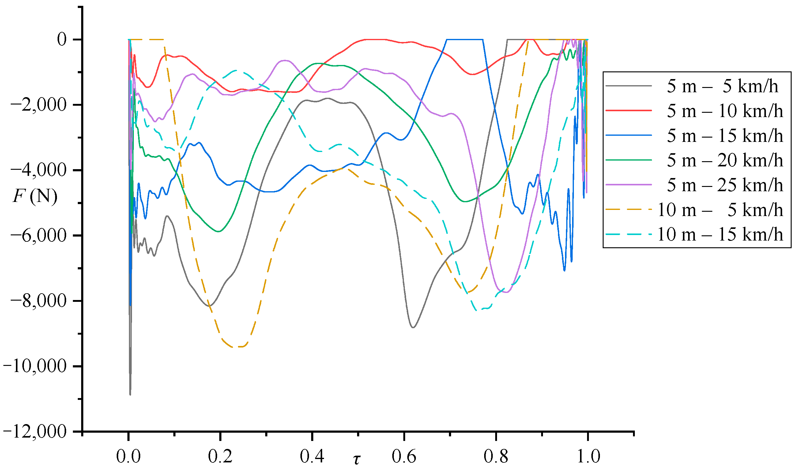
3.3. Standard Single-Valley Curve Model
The time-history curves of the contact forces of 10 m span under high-speed conditions have a single valley in the middle. This is also true for the contact force curves of 15 m span, regardless vehicle speed. In the same way as explained in the method in
Section 3.1 above, firstly, the identified contact force time-history curves were drawn in
Figure 6 with the unit duration parameter as the horizontal coordinate and the contact force as the vertical coordinate.
Using Equation (7), the standard single-valley curve as shown in
Figure 7 was obtained after fitting.
The coordinates of the control points obtained by fitting are shown in
Table 4, and the coordinates of the control points of the standard single-valley curve are shown in
Table 4.
3.4. Validation of Standard Single-Valley Curve
In order to verify whether the established single-valley curve can meet the requirements of engineering design under the corresponding working conditions, the simplified dynamics model of AERORail established by Li et al. [
5] and its Simulink simulation system were used for virtual loading. The working conditions involved in the simulation are shown in
Table 5.
The simulation parameters were again obtained from Li et al. [
5] with the obtained structure natural frequency, and take the linear density of the structure was
. After simulation, the mid-span deflection time under various working conditions was obtained as shown in
Figure 8.
We also recorded the simulation and experimental maximum deflection value of each calculation in
Figure 8, and calculated its relative error, and listed the results in
Table 6 and
Figure 9.
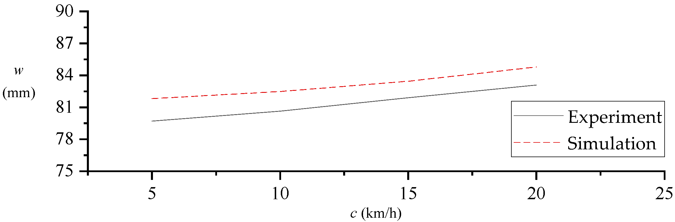
As can be seen from
Table 6 and
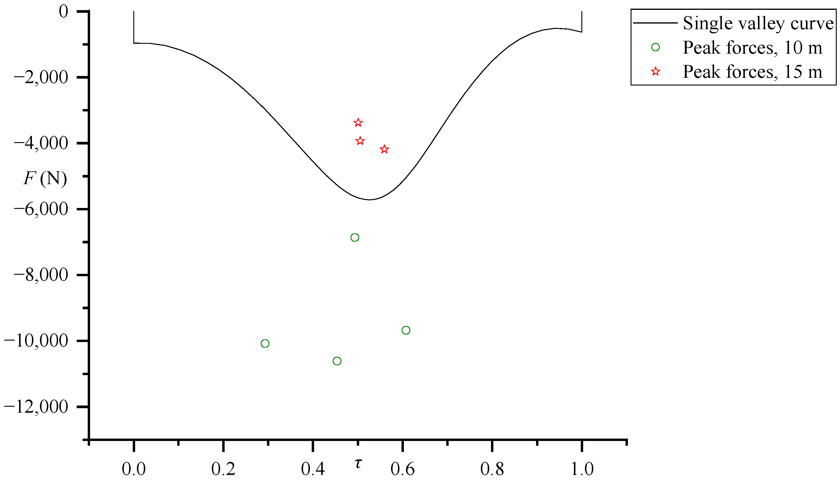
Figure 9, the numerical simulation results were relatively close to the actual experimental data at low speed, and the error was less than 3%. In all working conditions, the error remained stable, and the simulated value was stably large. This error was because the peak forces for the 15 m span were lower than the peak of the single-valley curve, as shown in
Figure 7. In all cases, the single-valley curve model had a good reference value for calculating the dynamic response of the AERORail structure with a span of 15 m, and good accuracy under all working conditions.
4. Comparative Analysis of Models
In terms of contact force identification results, the 10 m span AERORail structure was in the alternating range of double-valley and single-valley curves. The contact force time-history curve of the low-speed working condition presented a double-valley curve form, while the high-speed working condition presented a single-valley curve form. In order to clarify the most accurate ideal force model under different speed conditions over a 10 m span, and further study the difference between the calculation results of the standard double-valley curve and the standard single-valley curve over the same span and the same speed, this section used the simulation system to double-calculate the five speed conditions over a 10 m span by using two curve models respectively. The working conditions involved in the simulation are shown in
Table 7.
The simulation parameters were still the same as in Li et al. [
5]. The basic frequency of the structure was calculated and the quality of the structure line was taken as
. After simulation, the mid-span deflection time under various working conditions was obtained as shown in
Figure 10.
The maximum mid-span deflection obtained in
Figure 10 was compared with the maximum mid-span deflection measured in the experiment, and the results shown in
Table 8 and
Figure 11 were obtained.
As can be seen from
Table 8 and
Figure 11, the numerical simulation results of the standard single-valley curve were relatively close to the actual experimental data, with an error of less than 9%. The error was small at low speed, but increased with the increase of speed, and finally fluctuated around 8%. Again, this error was caused by the different peaks in the single-valley curve model and the samples, as illustrated in
Figure 7. The peaks for 10 m spans were higher than in the single-valley curve model, which led to the underestimation of deflection in the simulation.
The standard double-valley curve deviated greatly from the experimental value under all working conditions, and the simulated value was stably small, which indicates that the standard double-valley curve is not suitable for the calculation of a 10 m span, unless some correction is made. In general, the single-valley curve model has a certain reference value for calculating the dynamic response of the AERORail structure with a span of 10 m, and has relatively stable accuracy under all working conditions.
5. Calculation of High-Speed Working Conditions
In the design concept of the AERORail, the final design of the AERORail transportation system can reach 100~300 km/h. However, due to the limited conditions, the existing scale model experiment and experimental line experiment could not completely simulate such a high speed. Therefore, it was important to use the existing numerical simulation system and ideal load model to predict the possible high-speed working conditions and analyze the possible resonance of the bridge qualitatively. In this section, the standard single-valley curve model and standard double-valley curve model in
Section 2 were used to simulate 5 m, 10 m and 15 m span AERORail structures in the speed range of 40~300 km/h. The simulation calculation of a 30 m long AERORail structure without measured data was carried out.
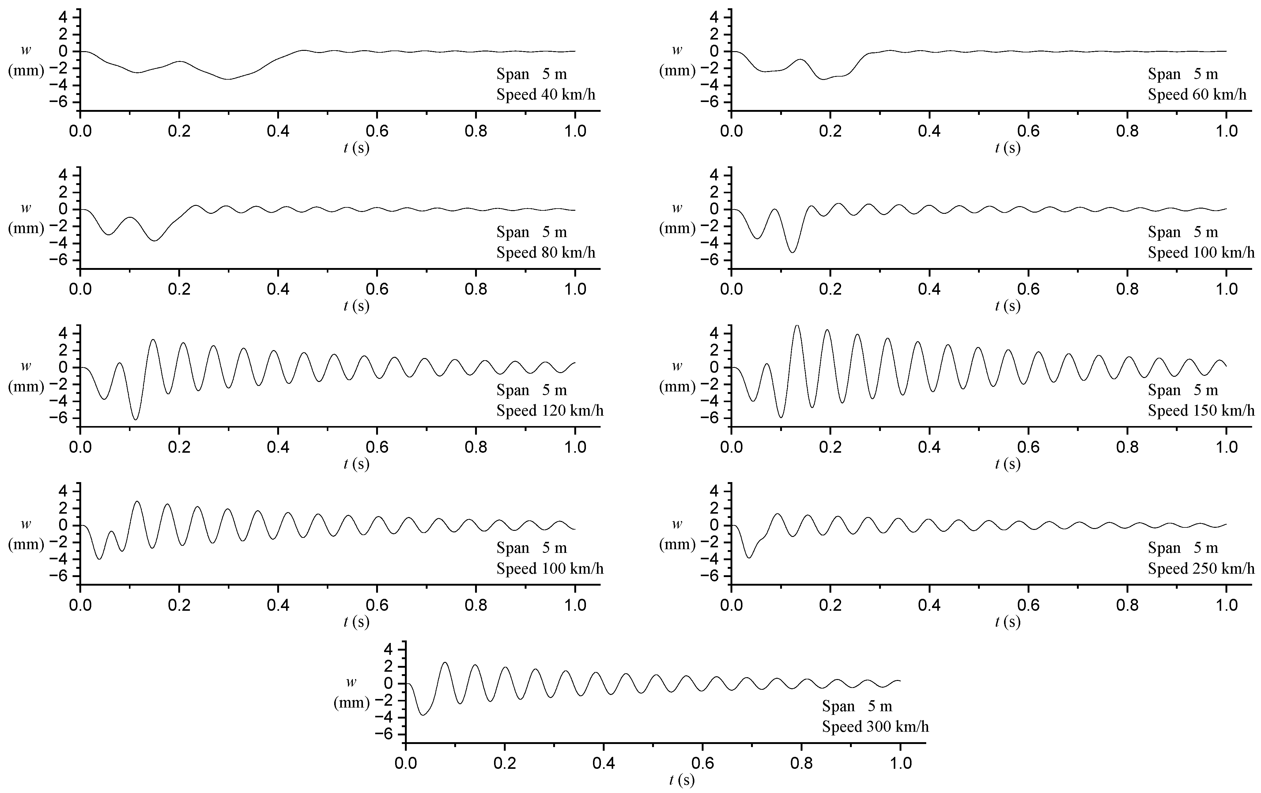
5.1. Short Span High-Speed Working Condition Simulation
The calculation parameters of 5 m, 10 m, and 15 m span AERORail structures were as described by Li et al. [
5] and
Section 2. The working conditions involved in the simulation are shown in
Table 9:
Considering that the standard double-valley curve model had satisfactory accuracy in the simulation of a 5 m span, the standard double-valley curve model was used to calculate the 5 m span AERORail structure. The calculated mid-span deflection-time curve is shown in
Figure 12.
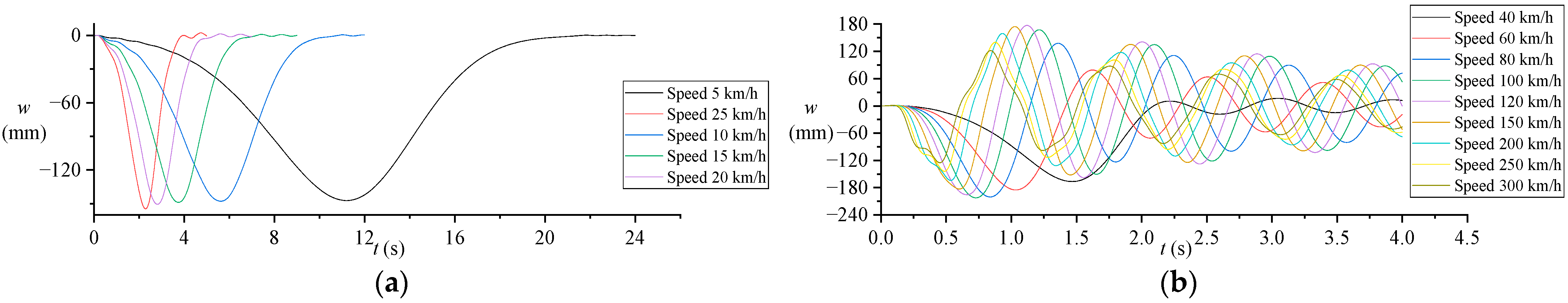
The simulation results in
Figure 12 showed the following. (1) With the increase of speed, the residual vibration amplitude retained by the AERORail structure after excitation increased continuously. (2) When the speed was greater than 100 km/h, the rebound in the AERORail span became more and more obvious. (3) With the increase of speed, the two extremes of deflection generated by the two-valley curve gradually approached each other and finally merged into a single extreme value (300 km/h, 3.73 mm). (4) The condition with the maximum deflection was not the condition with the highest speed, and the extreme deflection increased first and then became smaller with the increase of speed, reaching a maximum value of 6.19 mm around 120 km/h. (5) When the speed was greater than 250 km/h, the vibration response of the AERORail was close to damped free vibration.
According to the above results, the following conclusions can be drawn: (1) the dynamic response of a 5 m span under high-speed conditions gradually approached the response of a damped free vibration system with the increase of speed; (2) the resonance speed of a 5 m span was near 120 km/h; (3) the maximum dynamic deflection of a 5 m span under the action of a standard double-valley curve model was about 6.19 mm.
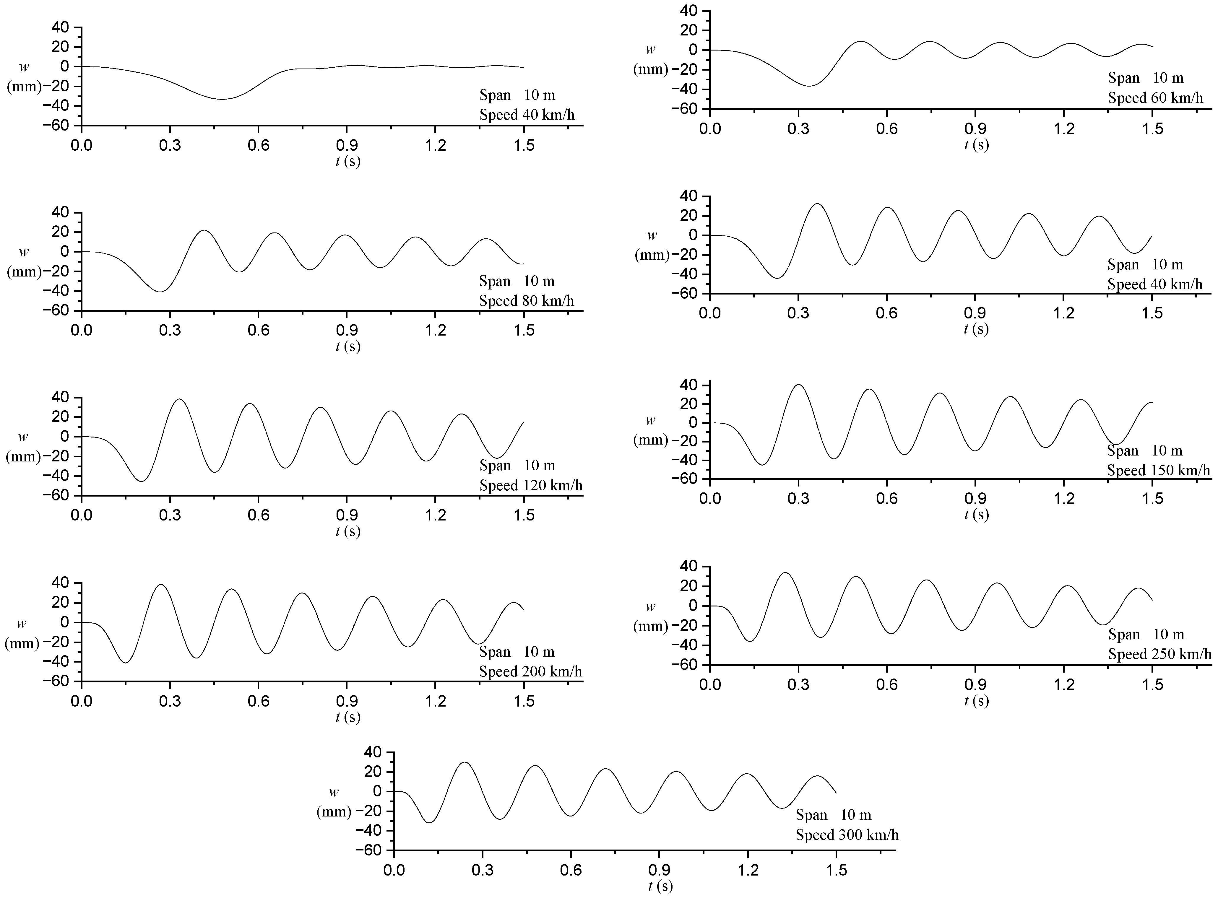
For the simulation of 10 m and 15 m spans, considering that the standard single-valley curve model had high calculation accuracy under these two span structures, and the contact force history curve itself was close to the single-valley curve shape under high-speed working conditions, the time force model used in the calculation of 10 m and 15 m spans was the standard single-valley curve model. The calculation results of the 10 m span under high-speed working conditions can be seen in
Figure 13.
The simulation results of the 10 m span high-speed working conditions had the following characteristics. (1) With the increase of speed, the residual vibration amplitude retained by the AERORail structure after excitation increased continuously. (2) When the speed was greater than 40 km/h, the rebound in the AERORail span became more and more obvious. (3) The condition of maximum deflection was similar to that of the 5 m span, but not the condition of highest speed. The extreme value of deflection increased first and then became smaller with the increase of speed, reaching a maximum value of 45.63 mm around 120 km/h. (4) When the speed was greater than 80 km/h, the vibration response of the AERORail was close to damped free vibration.
According to the above characteristics, the following conclusions can be drawn. (1) The dynamic response of the 10 m span under high-speed conditions gradually approached the response of a damped free vibration system with the increase of speed. (2) The resonant speed of the 10 m span was between 100 km/h and 150 km/h. (3) The maximum dynamic deflection of the 10 m span under the action of a standard single-valley curve model was not less than 45.63 mm.
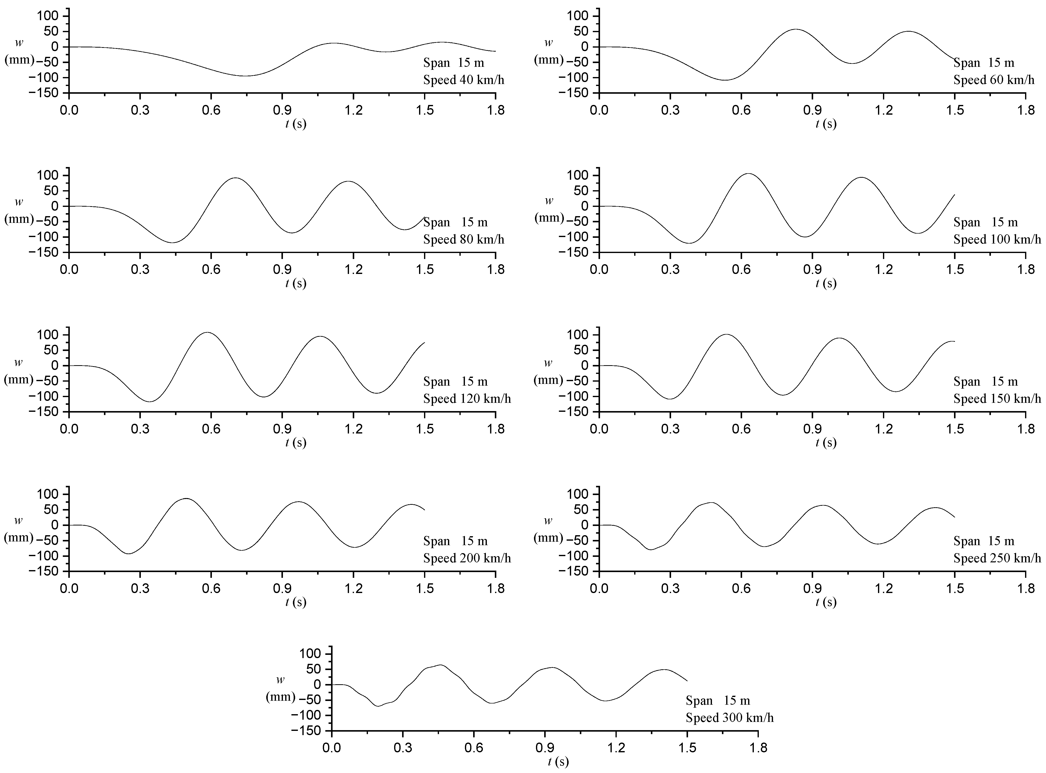
The calculation results of high-speed working conditions of the 15 m span can be seen in
Figure 14.
The simulation results of the 15 m span under high-speed conditions had the following characteristics. (1) With the increase of speed, the residual vibration amplitude retained by the AERORail structure after excitation increased first, and then decreased. (2) When the speed was greater than 40 km/h, the rebound in the AERORail span became more and more obvious. (3) The condition of maximum deflection was similar to that of the 5 m span, but not the condition of highest speed. The extreme value of deflection increased first and then became smaller with the increase of speed, reaching a maximum value of 120.48 mm at about 100 km/h. (4) When the speed was greater than 60 km/h, the vibration response of the AERORail was close to that of damped free vibration. (5) When the speed was greater than 250 km/h, the deflection curve started to exhibit local fluctuation.
5.2. Simulation of High Speed of 30 m Span
In order to study the dynamic characteristics of the AERORail structure with a larger span, this section carried out the simulation of a 30 m span AERORail structure to obtain its dynamic response under a moving point load. The magnitude of the point load was determined by the single-valley curve. This 30 m span of AERORail was similar to the 15 m span in structure. Three support rods were set on each side connecting the rail and the prestressed cable. The lengths of the three support rods were 40 cm, 54 cm, and 40 cm, respectively. The tensile force of the cable was the same as the tensile force (3 tons) used in the test line. Before simulation, the 30 m span structure was also established using the finite element model and its natural frequency was calculated (
Table 10).
The standard single-valley curve model load was used to test the 30 m span AERORail. The speed conditions involved in the calculation and the maximum span deflection within the working conditions are shown in
Table 11.
The mid-span deflection-time history curve of the 30 m span AERORail can be seen as shown in
Figure 15.
The simulation results of the 30 m span working conditions had the following characteristics. (1) With the increase of speed, the residual vibration amplitude retained by the AERORail structure after being excited first increased and then decreased. (2) When the speed was less than 25 km/h, the impact effect of dynamic load was not obvious, and the deflection of the AERORail was close to that of a static load. (3) When the speed was greater than 25 km/h, the dynamic response of the AERORail became obvious, and when the speed was greater than 40 km/h, the rebound in the span of the AERORail became more and more obvious. (4) The condition with the maximum deflection was similar to the conditions for 5 m, 10 m, and 15 m spans, but was not the condition with the highest speed. The extreme value of deflection increased first and then became smaller with the increase of speed, reaching a maximum value of 202.7 mm around 100 km/h. (5) When the speed was greater than 100 km/h, the vibration response of the AERORail was close to damped free vibration. (6) When the speed was greater than 150 km/h, the deflection curve began to show certain local fluctuation.
6. Conclusions
The present study explored a way to devise live load models for a novel transportation system called AERORail based on the vehicle–structure contact force identified from structure’s acceleration data. The identified contact forces were grouped and then fitted using Bezier curves and the least-squares method. The resultant two force models, namely the single-valley and double-valley curves, were validated in a Simulink model against the experiment data under five different vehicle speeds and three span lengths. The simulations showed that the proposed load model gave a good prediction of the mid-span deflection; therefore the established standard load models can be used for the dynamic analysis of AERORail. The conclusions are as follows.
(1) The live load for the lightweight AERORail can be obtained by fitting the identified contact force using Bezier curves. The resultant load curve can be used to predict the dynamic displacement response of the structure.
(2) The variation in span length leads to the different shape of the load curve. The load models for 5 m and 15 m span AERORails have one- and two-peak magnitudes, respectively. The variation of speed mainly affects the magnitude rather than the shape of the load curve.
Aside from the existing research on small-span AERORails and low-speed vehicles, this article also discusses the dynamic deflection of a 30 m AERORail with vehicle speed of 40–300 km/h. It was found from the simulation that:
(3) The resonant speed of the 30 m span was between 80 km/h and 100 km/h, which was less than that of the 5 m, 10 m, and 15 m spans. At speeds of about 150 km/h and above, higher-order vibration components began to appear. This phenomenon should be carefully considered in future design and research of AERORail.
The current study designed load models for AERORail. However, the methodology applied in the article can also benefit the load model study on other prestressed bridge structures.


