Magnetic Localization Method for Vehicles Based on Transformer

Abstract

Magnetic positioning is a promising technique for vehicles in Global Navigation Satellite System (GNSS)-denied scenarios. Traditional magnetic positioning methods resolve the position coordinates by calculating the similarity between the measured sequence and the sequence generated from the magnetic database with criteria such as the Mean Absolute Difference (MAD), PRODuct correlation (PROD), etc., which usually suffer from a high mismatch rate. To solve this problem, we propose a novel magnetic localization method for vehicles based on Transformer. In this paper, we cast the magnetic localization problem as a regression task, in which a neural network is trained by equidistant sequences to predict the current position. In addition, by adopting Transformer to perform magnetic localization of vehicles for the first time, magnetic features are extracted, and positional relationships are explored to guarantee positioning accuracy. The experimental results show that the proposed method can greatly improve the magnetic positioning accuracy, with an average improvement of approximately 2 m.

1. Introduction

Vehicle navigation services are essential for drivers, regardless of time, weather, or location conditions [1]. Currently, GNSS is spectacularly successful at generating accurate positioning solutions in most outdoor environments [2], whose standard horizontal positioning accuracy is 1.0–3.9 m [3]. However, this approach cannot satisfy the accuracy requirements of positioning tasks in GNSS-denied scenarios, due to the limited coverage ranges of networks and channel-fading issues. To solve this problem, various positioning systems [4], such as the Inertial Navigation System (INS), Wireless Fidelity (Wi-Fi), Bluetooth, and visual systems, have been studied. INS is capable of stand-alone positioning, but it can provide only relative results, and its accuracy decreases dramatically (tens of kilometers per hour at most [5]) as the operation time increases [6]. For Wi-Fi and Bluetooth, much effort is required to install and maintain a large amount of infrastructure, which makes the application of these technologies less attractive [7]. The accuracies that can typically be obtained with Wi-Fi and Bluetooth are 1–10 m and 2–15 m, respectively [8]. In recent years, visual positioning has become a popular approach due to its high precision (<5 m [9]). However, this method relies on complex image-matching algorithms, limiting its applicability to resource-constrained terminals, and it is easily affected by lighting conditions.

Compared to the positioning methods mentioned above, methods based on magnetic fields have been researched for a long time because of the following advantages. First, magnetic field-based positioning does not require any infrastructure, making such systems highly cost effective [10] because a magnetic field can be obtained anywhere on Earth [11]. Second, magnetic field signals are quite stable in the time domain, as opposed to radio frequency signals or sound waves, which is very important for matching-based methods [12]. Finally, magnetic fields offer all-weather availability in the sense that they are not affected by weather-related factors, such as light, rain, and snow.

However, magnetic signals are less distinguishable than Wi-Fi and Bluetooth signals, i.e., different positions may have similar magnetic observations, leading to a high probability of mismatch [13]. To improve the accuracy of magnetic localization, this paper innovatively proposes a magnetic localization method based on Transformer. The following contributions are made in this research.

• We propose a novel magnetic localization framework that is specifically designed for vehicles. On the one hand, assisted by mileage information, a magnetic sequence with equal distance intervals is used as the input. This solves the problem of inconsistent spatial scales due to speed and sampling frequency differences. On the other hand, we regard the magnetic positioning problem as a regression task in which a neural network serves as the regressor and directly outputs the desired position coordinates. This strategy is feasible for vehicles and ensures the accuracy of the positioning results because of the diversity of the input data.
• For the first time, we incorporate Transformer into the field of magnetic localization for vehicles. Transformer extracts magnetic features and explores the deep temporal position information of the input sequence, thus improving the positioning accuracy.

The remainder of this paper is organized as follows. We review the related work in Section 2. Section 3 introduces the proposed method in detail. Section 4 reports and discusses the results of several localization experiments. Finally, in the last section, we provide the main conclusions of this study and suggestions for future work.

2. Related Work

Many magnetic localization algorithms, such as Dynamic Time Warping (DTW), Magnetic Contour Matching (MAGCOM), filter-based approaches, machine learning and neural networks, are available. This section divides these methods into two categories, traditional methods and learning-based methods, and discusses their advantages and disadvantages in detail.

2.1. Traditional Methods

Traditional methods, including DTW, MAGCOM, and filter-based approaches, are fingerprinting methods that work by comparing a measured magnetic field sequence with magnetic sequences stored in a constructed database. They then find the most similar matching sequence to determine the current position [14]; this process is demonstrated in Figure 1.

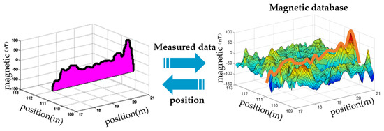
Figure 1. Principle of fingerprinting methods.

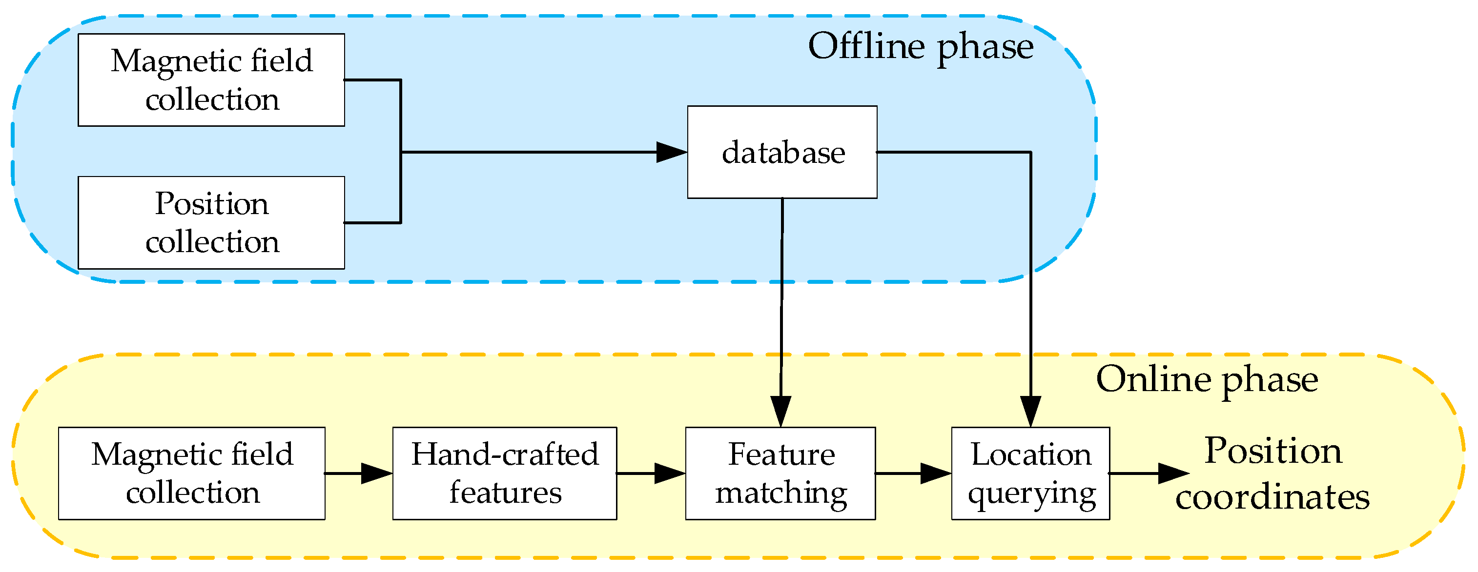
Specifically, this process consists of two phases, the offline and online phases [15], as shown in Figure 2. In the offline phase, a magnetic database with a certain granularity is built in the region of interest through measurement and interpolation. During the online phase, the collected magnetic sequences are manually extracted to features and matched with the fingerprints in the database. One of the above algorithms is used to calculate the most likely location.

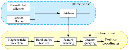
Figure 2. Framework of the traditional methods.

According to fingerprinting localization principles, it can be inferred that the errors in positioning results are attributed to two factors. On the one hand, the utilized database is usually quantized in a mesh grid form, and the magnetic field at each grid point comes from a single measurement [16], or the average of multiple measurements [17], or the interpolation of adjacent points [18]. Such a database consists of many isolated points, so it is not sufficient to fully describe the relationships between magnetic sequences and their positions. In addition, the magnetic field at each grid point is fixed, so it is insufficient to describe the noise distribution of the measurements because the measured magnetic field at a point is not a constant. On the other hand, feature-matching criteria are manually designed and cannot be used to precisely model the noise in measured data. Taking MAGCOM as an example, many comparison criteria are available, such as the PROD criterion, the Normalized PROD (NPROD) criterion, MAD criterion, and the Mean Standard Deviation (MSD) criterion [15]. These criteria are not comprehensive; they focus either on errors in a point-by-point manner or only on the overall trend, which easily causes mismatches. In a typical magnetic positioning application involving vehicles, the fingerprinting method can achieve an accuracy of 3.34 m (2σ).

2.2. Learning-Based Methods

Over the past ten years, learning-based methods have become a new trend [19,20], in which deep learning is superior to traditional machine learning and has already been applied to magnetic localization. Two aspects of deep learning-based methods compensate for the defects of traditional methods. On the one hand, a database is not used in a straightforward way but is instead used to generate training sets via random walking and data augmentation. In this way, the grid-like database used in traditional methods is replaced by a neural network, which emphasizes the relationships between magnetic sequences and locations and learns the noise distribution of measured data. On the other hand, benefiting from its data-driven design, a deep learning-based method can autonomously extract useful features for localization tasks due to its deep cascaded layers and strong fitting capabilities (rather than manually extracting features and designing matching criteria to implement positioning via traditional methods).

Many types of network structures have been proposed by researchers in the field of magnetic positioning, such as Convolutional Neural Networks (CNNs), Long Short-Term Memory (LSTM), Recurrent Neural Networks (RNNs), and Transformer. The authors of [21] used a standard CNN to classify extracted features in the spatial domain and exceeded 80% accuracy in a two-dimensional environment. In [22], CNNs were used to extract deep features, and correlations were utilized to obtain classification results. The results of a numerical simulation indicated that the mean matching rate surpassed 98.6%. Abid trained a CNN to transform a Recurrence Plot (RP) and a magnetic map into deep features. His method yielded location classification accuracy improvements of 3.05% and 3.64% [7] compared with another CNN-based system treating fingerprints relying on instantaneous magnetic field data [23]. In the same year, he proposed an improved CNN-based magnetic indoor positioning system using an attention mechanism, which outperformed the initial RP-based CNN but resulted in a much higher level of prediction latency [24]. The authors of [25] used an RNN to model magnetic time series, for which the input was a 3-dimensional magnetic vector and the output was 2-dimensional coordinates of the target location. This method provided average localization accuracy improvements of 57.5% and 74.6% over the results of the basic RNN model for medium- and large-scale testbeds, respectively. Wang introduced a LSTM-based recurrent RNN to handle localization problems with smartphones. The maximum location errors of this method are 8.2 m using the magnetic only [26]. Reference [27] attained improved accuracy by better modeling the magnetic relationships present in the time domain with a Bidirectional LSTM (Bi-LSTM) structure. This method achieved positioning errors that were 88.6% and 76% less than those of the DTW method on two datasets. Wang leveraged different scales to segment magnetic data and extracted magnetic sequence features at the corresponding scales through Transformer [28]. Moreover, multiple scale features were fused for positioning. Compared to typical magnetic field positioning methods, 90% of the positioning errors of this approach decreased by 13.79–60.73%. Reference [29] built Generative Adversarial Networks (GANs) to augment their training set, unburdening the data collection process and leading to a mean localization accuracy improvement of 9.66% over the conventional semi-supervised localization algorithm.

Although the accuracy of the positioning results has improved to a certain extent, most of the abovementioned neural networks were designed for pedestrian positioning. In general, training sets are generated by limited measured data to decrease the difficulty of human collection, which inevitably introduces errors and limits the performance of the network. In addition, the spatial inconsistency of magnetic data caused by different speeds makes neural networks difficult to train; thus, the accuracy improvement achieved by the results is relatively limited.

In summary, according to the magnetic localization algorithms mentioned above, deep learning-based methods greatly improve upon the positioning accuracy of traditional approaches by better extracting features and performing the matching process. However, better neural network models that incorporate the characteristics of vehicle positioning to achieve improved performance must be explored.

3. Methods

Compared to magnetic pedestrian positioning, the use of magnetic fields for vehicles has some beneficial characteristics. First, mileage information can be integrated based on the speed obtained from the speed sensor with which every vehicle is equipped [15]. This information can be used to transform a magnetic time series into a spatial sequence, which avoids the spatial inconsistency problem of magnetic data caused by the different speeds of vehicles and the different sampling rates of magnetometers. Second, unlike human data collection, which has a high cost, vehicle data collection is more efficient. Therefore, it is easier to construct a training set from multiple actual measured data, which is more realistic than obtaining pedestrian positioning data through random walks and data augmentation. Third, three-axis magnetic fields can be directly used after eliminating the carrier interference because of the repetitive nature of the postures of vehicles travelling on the same path.

3.1. System Architecture

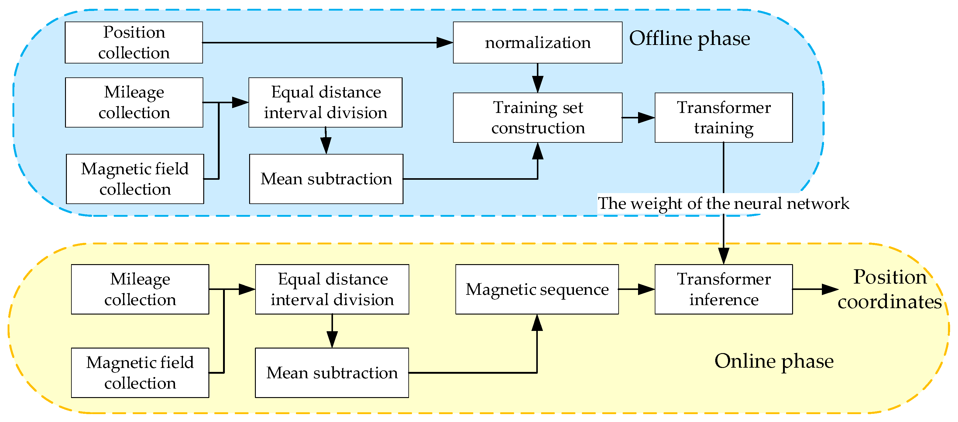
Based on the abovementioned vehicle characteristics, we design the architecture shown in Figure 3, which consists of an offline phase and an online phase. During the offline phase, the three-axis magnetic field vectors within a certain distance are collected and divided into equal distance intervals based on their mileage, which ensures that the sequence is independent of the vehicle’s speed and magnetometer’s sampling rates. Moreover, the true positions are collected as the labels of the training set, which are normalized to 0~1 to easily train the Transformer model. Thus, using multiple collected data, a training set that includes numerous sequences consisting of the magnetic field and the corresponding positions of a fixed number of points is generated. During the online phase, the trained Transformer model predicts the position coordinates with equidistant magnetic sequences obtained in the same way as those acquired in the offline phase. Notably, the mean magnetic field within a sequence must be subtracted to prevent the influence of carrier interference.

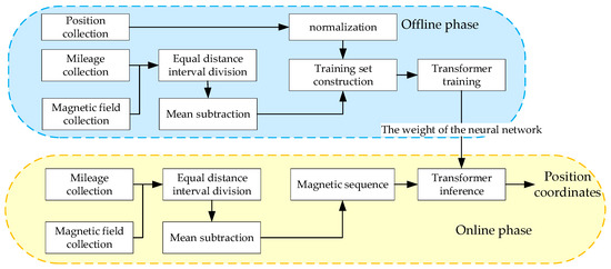
Figure 3. The architecture of our proposed magnetic localization method.

According to the above procedure, the input of the proposed method is a fixed-length three-axis magnetic sequence whose size is W × 3, where W is the number of points in the sequence, which is calculated by the whole length of the sequence L and the spatial interval d:

$$W=L/d$$

(1)

where L is related to the size of the target area. As a matter of experience, short sequences (approximately ten meters) can achieve accurate results for a small area; conversely, a larger area requires longer sequences (tens to thousands of meters) to distinguish different positions. This is because the larger the area is, the greater the possibility of short sequences with similar shapes, making it easier to cause mismatches. In addition, d represents the spatial resolution, which is related to the fluctuation degree of the magnetic field in the environment. For an indoor or a densely built environment, the magnetic field varies greatly in the spatial domain, so d needs to be set to a small value (0.5 m to 1 m).

Regarding the output, the proposed method aims to estimate the 2-dimensional coordinates of the current position (x,y), which is the last point in the sequence based on the current and past magnetic field values.

3.2. Transformer Model Structure

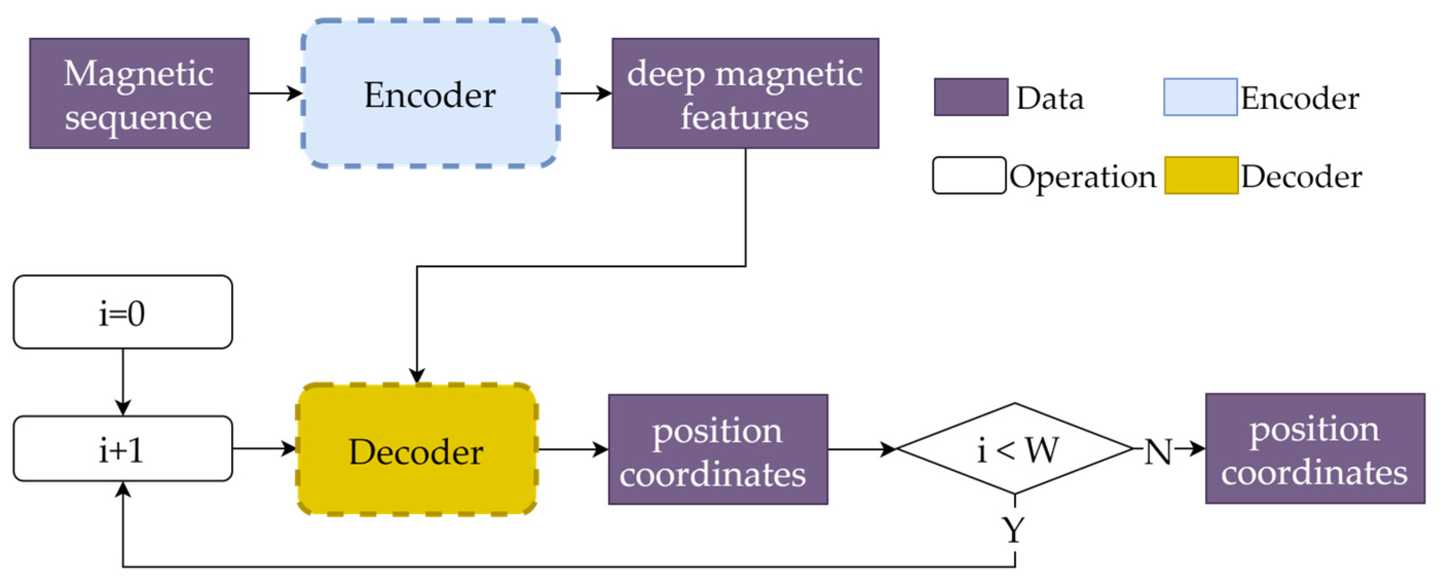
Figure 4 shows the proposed model structure, which consists of two parts: an encoder and a decoder. The encoder is responsible for extracting magnetic features from sequences. The decoder aims to predict the current location by exploring the deep temporal position features with the help of the features extracted from the encoder.

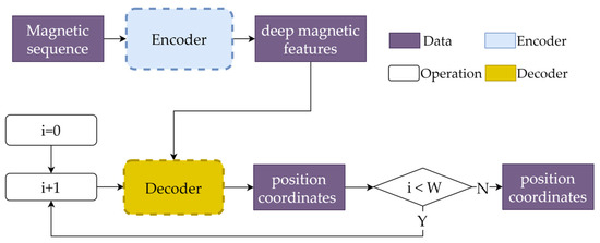
Figure 4. The structure of the proposed Transformer model.

The magnetic field sequence has a size of [B,W,3], where B and W represent the numbers of batches and points contained in the input sequences, respectively, and 3 represents the three axes of the magnetic field. After executing the encoder, deep magnetic features with shapes of [B,W,D] are extracted, where D is the dimensionality of the deep features.

The decoder is calculated W times. At each step i, the previous positions, along with the deep magnetic features extracted by the encoder, are fed into the decoder. In this way, the final position is recursively predicted. Since we focus only on the current position, which is the last point within the sequence, once i = W, the last position is pushed out as the final result. Next, we describe the encoder and decoder in detail.

3.2.1. Encoder

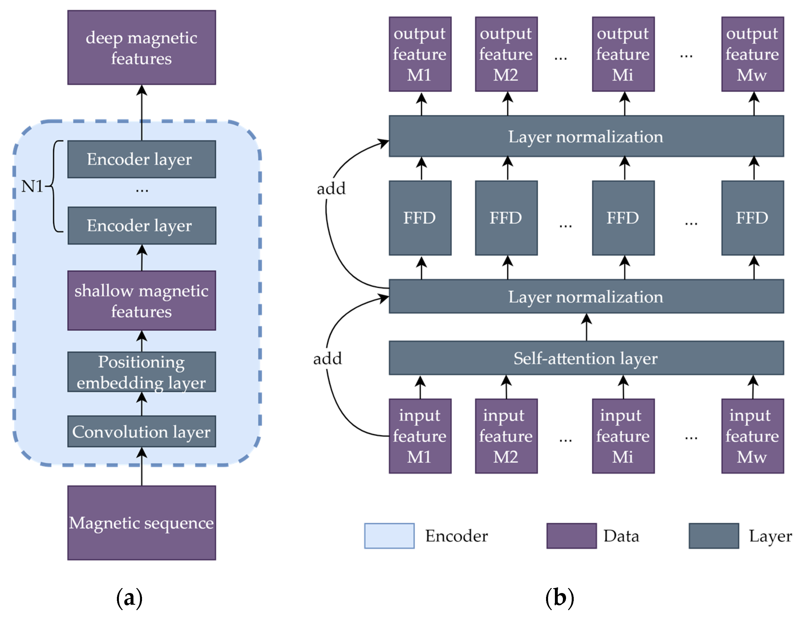
The structure of the encoder is shown in Figure 5a. First, shallow magnetic features are extracted from the given magnetic sequence by passing through a convolutional layer and a positional embedding layer [30]. Thus, the dimensionality of the original magnetic sequence is expanded from 3 to D. Then, the shallow features are fed into N₁ Transformer encoder layers and become deep features with shapes of [B,W,D]. Each Transformer encoder layer possesses the same structure as that of the standard Transformer [30], which is shown in Figure 5b, including one self-attention layer, one FeedForwarD (FFD) layer, two layer normalization operations, and several residual connections.

Figure 5. The structures of the (a) encoder and (b) encoder layers.

Self-Attention Layer: The self-attention layer is the core component of the encoder layer; it enables the encoder to extract useful temporal information. The self-attention layer is based on a multihead attention mechanism, which is an advanced version of the attention mechanism formulated in Equation (2):

$$\mathrm{Attention}(Q,K,V)=\mathrm{softmax}(\frac{Q{K}^T}{\sqrt{d_k}})V$$

(2)

where $Q\in R^{Q_t\times d_k}$, $K\in R^{K_t\times d_k}$, and $V\in R^{V_t\times d_k}$ are the query, key, and value matrices, respectively. Q_t, K_t, and V_t are the numbers of queries, keys, and values, respectively, and d_k is the second dimension. Q, K, and V can be easily computed by a combination of linear transformation and concatenation for every timestamp.

The multihead attention mechanism can be expressed as shown in Equation (3):

$$\mathrm{MultiHead}(Q,K,V)=\mathrm{concat}(\mathrm{Attention}(Q_i,K_i,V_i))W_{D\times D}^O$$

(3)

where $Q_i=Q{W}_{D\times (D/h)}^Q$, $K_i=K{W}_{D\times (D/h)}^K$, and $V_i=V{W}_{D\times (D/h)}^V$. $W_{D\times (D/h)}^Q$, $W_{D\times (D/h)}^K$, and $W_{D\times (D/h)}^V$ represent the weight matrices for Q, K, and V, respectively, with shapes of D × (D/h), where h is the number of heads, and concat(*) is the concatenation operation. $W_{D\times D}^O$ is the final output matrix with a shape of D × D.

Therefore, the self-attention mechanism can be written as shown in Equation (4):

$$\{\begin{array}{c}\mathrm{SelfAtt}(X)=\mathrm{MultiHead}(Q,K,V)\\ Q=\mathrm{concat}(W^Q{X}_i)\begin{array}{cc}\begin{array}{cc}& \end{array}& i\in [1,W]\end{array}\\ K=\mathrm{concat}(W^K{X}_i)\begin{array}{cc}\begin{array}{cc}& \end{array}& i\in [1,W]\end{array}\\ V=\mathrm{concat}(W^V{X}_i)\begin{array}{cc}\begin{array}{cc}& \end{array}& i\in [1,W]\end{array}\end{array}$$

(4)

where X is the input of the self-attention layer, which can be viewed as the magnetic features extracted from the given sequence, and X_i is the i-th magnetic feature in the sequence.

FFD Layer: Among the above-described layers, only the FFD layer is time-independent, which means that M_i, the i-th feature, is determined only by the i-th input. The other layers evaluate all the inputs of the entire sequence to compute the layer outputs.

Layer Normalization: Layer normalization is a common type of normalization operation used in deep learning [31]; it is applied after implementing a simple addition operation involving the current data stream and the data stream connected with a residual connection.

3.2.2. Decoder

As shown in Figure 6, the deep magnetic features extracted from the encoder, along with the previous positions, are inputted into the decoder. Similar to the encoder, shallow position features with sizes of [B,i,D] are extracted from the previous positions by a simple convolutional layer and a positional embedding layer, where i ∈ [1,W]. The attention mask is a predefined tensor, which is described in detail below. Then, the position features pass through N₂ Transformer decoder layers and are transformed into deep position features. Finally, the position features are projected to the coordinates of the target position (x,y) in 2 dimensions.

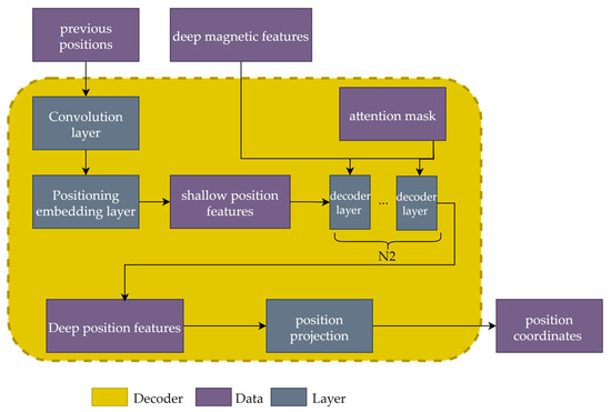
Figure 6. Structure of the decoder.

Since the decoder relies on the previous positioning results, it is implemented in a recurrent manner to obtain the final location. Specifically, given a new magnetic sequence, the position of the first point in this sequence is predicted first by executing the decoder once, where [−1, −1] is chosen as the initialized input. Then, the position of the second point can be computed by running the decoder again. This recursive procedure can be applied to the entire sequence. Therefore, in the online phase, the decoder is operated W times to obtain the final position.

The decoder layers have the same structure as those in [30] and are slightly different from the encoder layers, as shown in Figure 7. The decoder layers replace the self-attention layer with a masked self-attention layer and have an extra cross-attention layer.

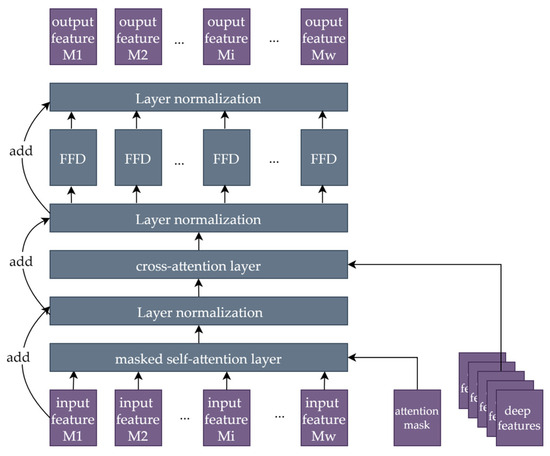
Figure 7. The structure of a decoder layer.

Masked Self-Attention Layer: This layer is a variant of the self-attention layer. The only difference is that an attention mask Mask_att with a size of [i, i] is added to the attention computation. Mask_att is an upper triangular matrix, and Equation (5) shows an example of Mask_att when i = 5.

$$Mas{k}_{att}=\left[\begin{array}{ccccc}0& -\inf & -\inf & -\inf & -\inf \\ 0& 0& -\inf & -\inf & -\inf \\ 0& 0& 0& -\inf & -\inf \\ 0& 0& 0& 0& -\inf \\ 0& 0& 0& 0& 0\end{array}\right]$$

(5)

This mask is applied in the attention computation, as shown in Equation (6):

$$\mathrm{MaskAttention}(Q,K,V,Mas{k}_{att})=\mathrm{softmax}(\frac{Q{K}^T}{\sqrt{d_k}}+Mas{k}_{att})V$$

(6)

For point k in the input sequence, -inf means that the attention response is not activated from a point with i > k, and the attention response from i ≤ k remains. This design ensures that only the previous input contributes to the output at the current moment and that a future input does not influence past outputs.

Cross-Attention Layer: This layer differs from self-attention layers in terms of the sources of Q, K, and V. In the self-attention layer, Q, K, and V come from the same sources as those of the input. However, in the cross-attention layer, Q is generated by the input as well, while K and V are generated by the deep magnetic features extracted from the encoder.

3.3. Training Strategy

Network training is performed during the offline phase. The neural network is fed with paired training samples to update its weights via gradient backpropagation. Once the training process is complete, the weights are fixed and can be used for the online phase.

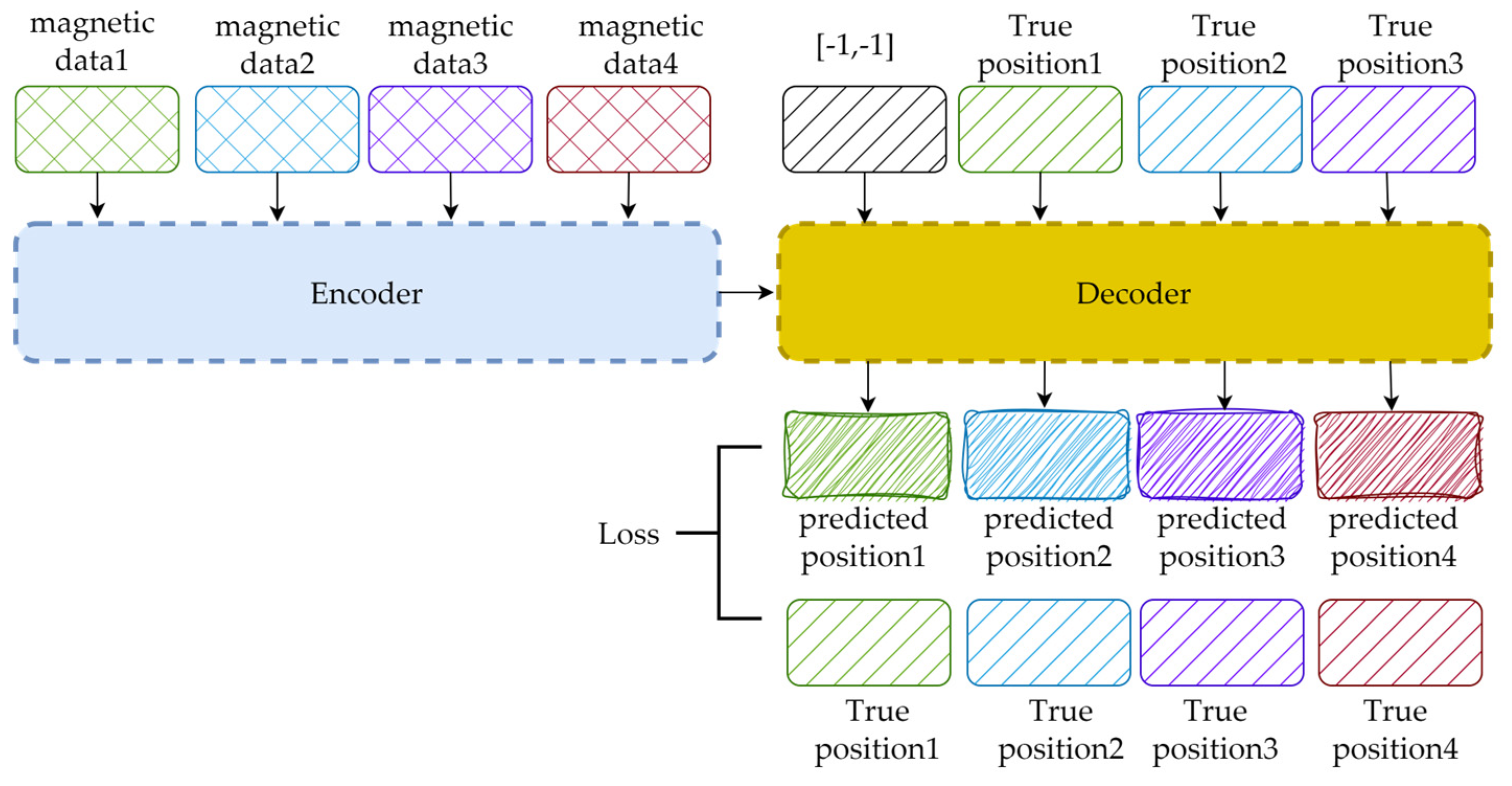
Figure 8 shows a simple example with B = 1 and W = 4. Considering the speed and stability of the training process, the data flow that occurs during network training is slightly different from that in the inference phase, which can be summarized as follows. First, the magnetic data are input altogether instead of in order, so the decoder runs only once instead of W times. Second, the input of the decoder is a one-step right-shifted version of the true position; [−1, −1] is padded to the first point in the sequence. Finally, during the online phase, we only focus on the position of the last point within the sequence. In contrast, every predicted position matters during training. The losses between the predicted and true positions of every point in the sequence are computed via gradient backpropagation.

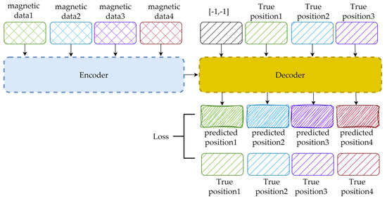
Figure 8. The data flow occurring during the training process.

The loss function consists of two parts: a location loss and a movement loss. The location loss is a simple Mean Squared Error (MSE) loss, and the movement loss can be written as Equation (7):

$$los{s}_{movement}=\frac{1}{W-1}{\displaystyle \sum _{i=1}^W\mathrm{MSE}(P_{i+1}-P_i,T{P}_{i+1}-T{P}_i)}$$

(7)

where P_i and TP_i represent the predicted position and true position at i, respectively. The final loss is the sum of the location and movement losses.

To improve the convergence of the model, a warm-up strategy is introduced during training. The learning rate starts at 1.2 × 10⁻⁵ and gradually increases to 1 × 10⁻⁴ after 5000 steps. Then, the learning rate decreases linearly to almost 0 when the training process is finished.

4. Experiments and Discussions

In this section, we report experiments conducted to evaluate the proposed magnetic localization method.

4.1. Experimental Setup

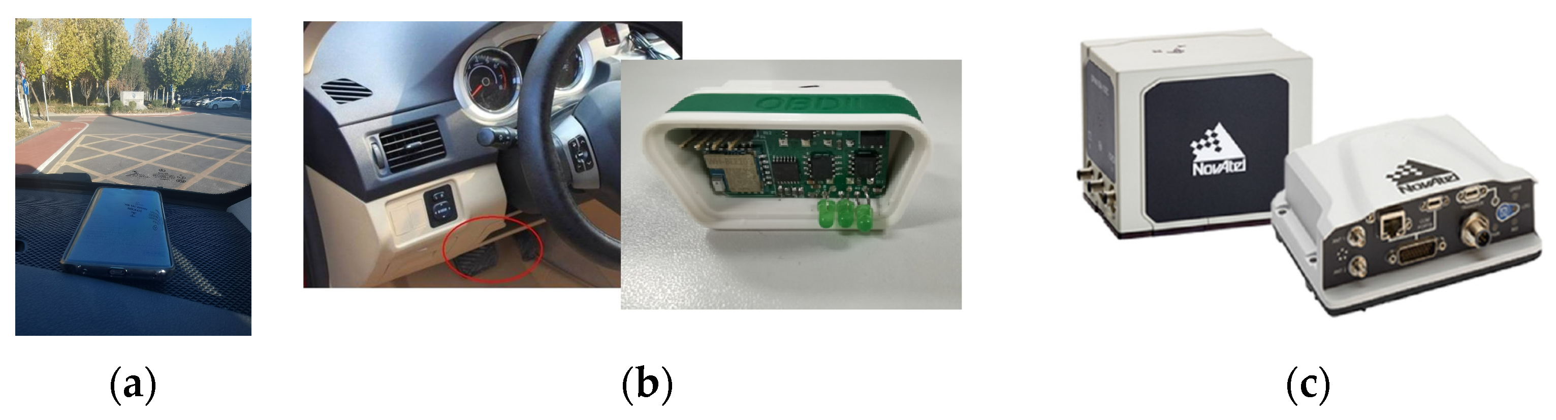
Dataset: Considering that the existing publicly available magnetic datasets [32,33,34,35,36] are not suitable for our application, we collected a dataset ourselves to evaluate the proposed method. Magnetic field data were collected from a Huawei Mate 20 Pro smartphone fixed on a vehicle, as shown in Figure 9a, and mileages were integrated by the velocities obtained from the On-Board Diagnostic (OBD) system of the vehicle. A self-developed module accessed the interface of the OBD system and transmitted the velocity to the smartphone, as shown in Figure 9b. The statistical results showed that the error of the integrated mileage was approximately 1% after calibration. Additionally, a differential GNSS/INS system called SPAN-ISA-100C (NovAtel Inc., Calgary, Canada) with a horizontal positioning accuracy better than 0.04 m/60 s [37] was used to evaluate the positioning accuracy of the magnetic localization results, as shown in Figure 9c.

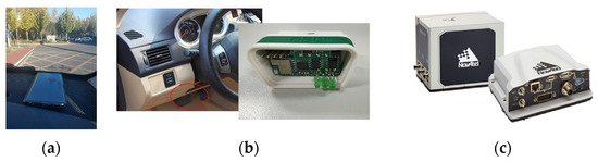
Figure 9. Equipment used in the experiment: (a) smartphone, (b) OBD system interface and self-developed module, (c) SPAN-ISA-100C.

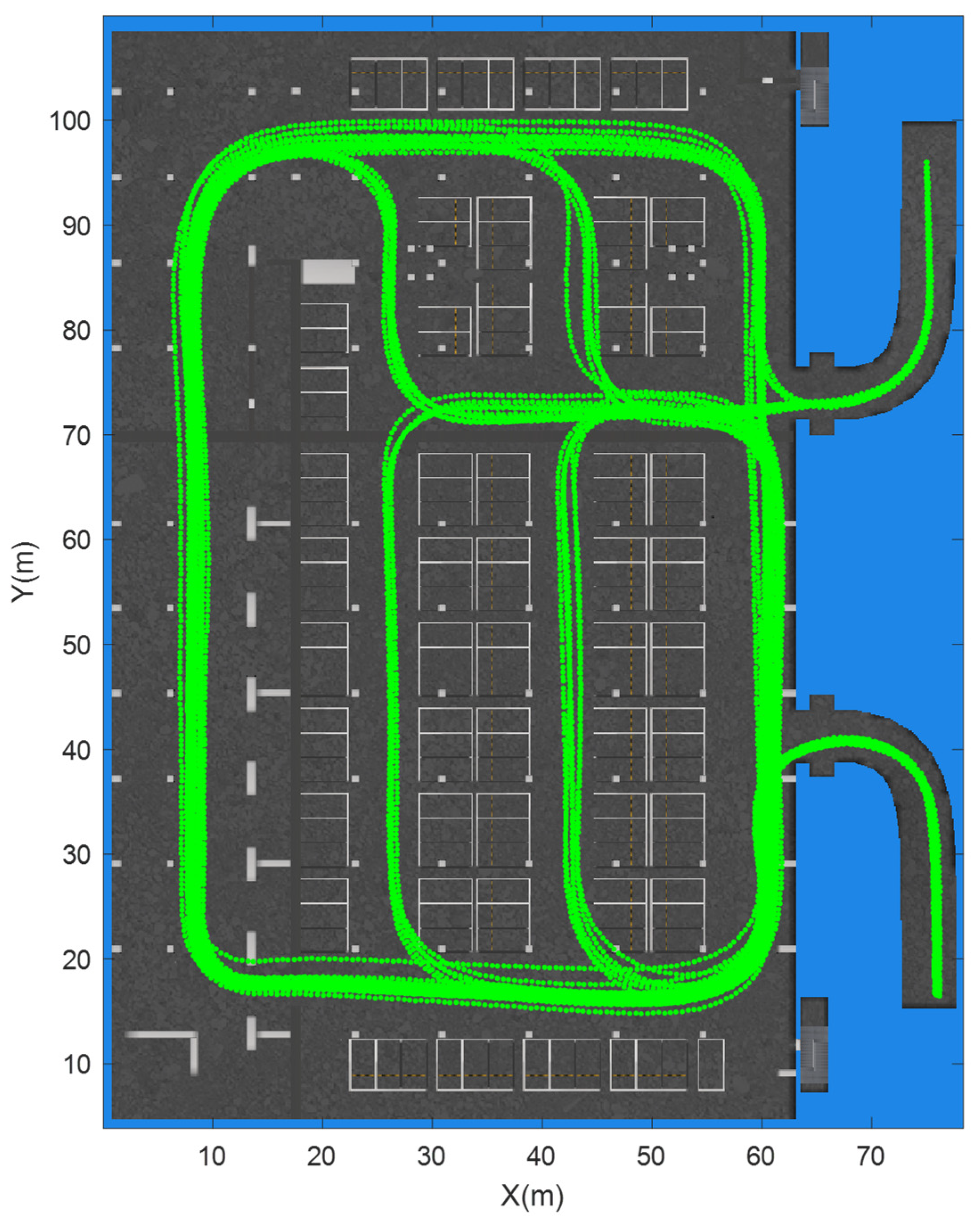
The test environment was a parking garage at the Beijing New Technology Base of the Chinese Academy of Sciences, which has an area of approximately 80 × 110 m², as shown in Figure 10. We collected 35 tracks, with a total length of 8094 m, as shown by the green lines in Figure 10; each track was divided into numerous sequences with diverse sequence lengths. In this section, we set the sequence length L from 5 m to 15 m, with a spatial interval d of 0.5 m, so W ranged from 10 to 30, as calculated by Equation (1). Taking a W of 14 as an example, the total number of sequences was 15,733, and 27 tracks containing 12,130 samples were selected for training (accounting for approximately 77%), while the remaining 8 tracks containing 3603 samples were used for evaluation purposes.

Figure 10. The data were collected from the test environment.

Model: We set the feature dimensionality D to 256, and the numbers of encoder layers N₁ and decoder layers N₂ were both 4. In addition, the training batch size was set to 1, and the number of training epochs was set to 30. The weighted Adaptive Moment Estimation (AdamW) optimizer was used with parameters of [0.9, 0.999]. Our model was implemented with the PyTorch library, and the detailed configuration is shown in Table 1.

Table 1. Experimental configuration.

Category	Machine/Tools
CPU	Intel(R) Core(TM) i9-12900H CPU (Intel Corporation, Santa Clara, CA, USA)
GPU	NVIDIA GeForce RTX 2050 GPU (NVIDIA, Santa Clara, CA, USA)
Operating System	Windows 11
Language	Python 3.8
Library	PyTorch 1.13

4.2. Positioning Performance

Several experiments were conducted to prove the superiority of our method over the traditional approaches.

Table 2 and Table 3 show the mean and maximum positioning errors, respectively, induced for sequences with different lengths concerning 8 tracks, which were obtained on the evaluation dataset by our method and three other methods, including the method in [12,27] and the traditional MAGCOM method. Considering that the dataset used in this work is different from the datasets used in [12,27], we reconstructed the same network structure as that in [12,27], respectively. For MAGCOM, we used an MAD metric, which has high accuracy and a simple calculation process as shown in Equation (8):

$${\mathrm{MAD}}_{AB}=\frac{1}{3W}{\displaystyle \sum _{i=1}^3{\displaystyle \sum _{k=1}^W\left[\left|\left(A_k^i-mean(A^i)\right)-\left(B_k^i-mean(B^i)\right)\right|\right]}}$$

(8)

where A is the measured sequence, B is a possible matching sequence of length W in the constructed database, i is an index representing each axis of a magnetic field vector, and k is an index representing the k-th point in the sequence.

Table 2. The mean errors (m) induced by sequences of different lengths when executing the proposed method and other methods on various evaluation data.

Method	Sequence Length	Evaluation Data
		1	2	3	4	5	6	7	8
Proposed method	5 m	2.31	4.66	1.58	2.15	2.60	2.80	4.05	1.93
	6 m	1.08	1.48	0.71	0.85	0.87	1.10	1.54	0.86
	7 m	0.98	1.29	0.58	0.71	0.71	1.00	1.34	0.72
	8 m	0.95	1.04	0.56	0.74	0.72	0.89	1.15	0.61
	9 m	0.92	1.04	0.50	0.60	0.56	0.86	1.21	0.68
	10 m	0.90	0.98	0.52	0.63	0.58	0.83	1.12	0.68
	11 m	0.87	1.02	0.47	0.63	0.60	0.79	1.07	0.51
	12 m	0.93	1.06	0.51	0.60	0.58	0.87	1.13	0.61
	13 m	0.85	0.99	0.39	0.55	0.51	0.75	1.06	0.56
	14 m	0.84	0.98	0.42	0.63	0.57	0.77	1.02	0.54
	15 m	0.82	0.93	0.40	0.60	0.55	0.70	1.06	0.62
Traditional MAGCOM method using the MAD metric	5 m	9.70	6.39	9.65	8.54	9.42	7.64	8.18	10.80
	6 m	7.15	4.77	8.04	7.10	6.27	5.84	5.62	8.89
	7 m	4.85	4.01	6.12	5.32	4.81	4.43	5.28	7.13
	8 m	3.48	3.29	4.48	4.25	4.07	3.74	4.70	5.28
	9 m	2.87	2.90	3.16	2.84	3.11	2.99	4.08	3.68
	10 m	2.00	2.52	2.05	2.50	2.38	2.23	3.46	2.25
	11 m	1.90	2.12	1.87	2.21	1.92	1.81	2.97	2.01
	12 m	1.78	2.15	1.74	1.88	1.83	1.81	2.10	1.93
	13 m	1.77	1.99	1.74	1.87	1.83	1.81	2.12	1.92
	14 m	1.77	1.91	1.74	1.87	1.83	1.81	2.12	1.92
	15 m	1.76	1.89	1.75	1.87	1.83	1.81	2.12	1.90
Method in [12]	5 m	5.64	6.22	4.69	5.08	4.88	5.07	6.46	4.59
	6 m	4.03	5.06	3.56	4.22	4.14	4.38	5.69	4.06
	7 m	3.80	4.20	2.91	3.80	3.58	3.64	4.35	3.29
	8 m	2.97	3.80	2.75	3.42	2.98	3.17	4.10	2.94
	9 m	2.79	3.31	2.49	2.92	2.74	2.98	3.63	2.58
	10 m	2.76	3.57	2.48	2.99	2.59	2.74	3.42	2.54
	11 m	2.23	3.41	1.87	2.60	2.44	2.59	2.98	2.07
	12 m	2.50	3.28	1.96	2.60	2.40	2.53	3.17	1.99
	13 m	2.58	3.06	2.14	2.63	2.41	2.62	3.19	2.30
	14 m	2.44	3.18	1.97	2.40	2.31	2.49	2.72	2.15
	15 m	2.35	3.23	1.92	2.25	2.18	2.31	2.85	1.94
Method in [27]	5 m	2.65	2.80	1.22	2.35	1.70	1.74	4.02	1.82
	6 m	1.88	2.67	1.22	2.02	1.71	1.76	3.16	1.54
	7 m	1.88	2.64	1.18	2.06	1.69	1.76	3.12	1.54
	8 m	1.83	2.66	1.19	2.06	1.67	1.73	3.04	1.53
	9 m	1.85	2.63	1.15	2.09	1.66	1.79	3.05	1.51
	10 m	1.86	2.69	1.16	2.13	1.65	1.79	3.01	1.51
	11 m	1.84	2.70	1.16	2.13	1.67	1.74	2.99	1.50
	12 m	1.85	2.64	1.21	2.15	1.66	1.75	3.08	1.49
	13 m	1.87	2.63	1.22	2.12	1.65	1.81	3.04	1.50
	14 m	1.91	2.63	1.14	2.10	1.66	1.74	3.07	1.51
	15 m	1.89	2.74	1.26	2.23	1.78	1.98	3.15	1.49

Table 3. The maximum errors (m) induced by sequences of different lengths when using the proposed method and other methods on various evaluation data.

Method	Sequence Length	Evaluation Data
		1	2	3	4	5	6	7	8
Proposed method	5 m	37.91	57.29	18.05	30.95	44.33	91.94	33.27	19.74
	6 m	5.00	6.53	2.10	8.72	6.51	6.29	9.09	2.16
	7 m	2.69	4.20	1.84	3.50	3.28	3.22	4.63	1.82
Traditional MAGCOM method using the MAD metric	5 m	91.07	81.57	91.00	90.67	90.39	91.17	86.08	91.04
	6 m	91.17	62.92	91.00	90.36	90.53	91.17	73.36	91.14
	7 m	91.17	62.40	90.70	90.02	90.53	90.86	73.92	90.83
	8 m	72.91	45.75	72.67	74.04	89.88	72.85	64.61	90.49
	9 m	76.94	44.72	72.82	71.93	83.71	72.77	64.61	72.97
	10 m	15.37	43.35	15.49	52.45	83.86	51.97	62.36	15.41
	11 m	15.37	26.34	15.01	52.89	14.62	3.06	62.36	15.37
	12 m	2.66	26.34	2.33	2.67	2.54	2.96	15.69	2.84
	13 m	2.66	26.34	2.33	2.60	2.54	2.99	15.24	2.84
	14 m	2.46	7.18	2.33	2.60	2.54	2.83	15.24	2.84
	15 m	2.66	7.29	2.33	2.60	2.54	2.62	14.77	2.89
Method in [12]	5 m	48.59	27.55	18.06	27.34	25.59	24.99	33.02	22.47
	6 m	24.80	24.84	9.57	24.40	20.26	24.64	23.04	16.43
	7 m	27.66	17.72	9.53	36.54	17.72	16.33	24.08	13.00
	8 m	10.47	22.50	9.78	23.01	10.49	11.89	25.50	10.02
	9 m	11.07	14.69	10.25	15.84	13.00	13.77	16.29	10.91
	10 m	10.42	13.24	9.88	32.35	11.65	10.75	20.50	9.54
	11 m	9.23	15.53	4.96	17.05	14.83	11.79	12.84	6.60
	12 m	11.83	13.77	7.45	17.76	9.56	9.70	11.31	7.81
	13 m	15.60	13.66	8.71	15.50	13.92	11.21	9.87	9.82
	14 m	15.50	11.85	6.26	11.20	12.06	10.29	9.49	6.67
	15 m	11.19	17.35	13.14	14.75	12.00	9.47	13.31	14.07
Method in [27]	5 m	84.06	13.93	1.39	50.21	2.95	2.28	122.87	38.26
	6 m	3.07	13.93	1.52	2.82	2.81	2.33	14.03	1.58
	7 m	3.19	3.51	1.61	3.02	2.77	2.60	13.11	1.49
	8 m	2.44	3.51	1.39	3.02	2.69	2.33	3.52	1.70

As shown in Table 2, the mean positioning accuracies of our method were greater than those of traditional MAGCOM methods and the method in [12] with the same sequence length for all the evaluation data, and an average improvement of 2.67 m (70.08%) and 2.26 m (70.73%) were observed. In addition, we compared our method with the method in [27]. In most cases, the results indicated that the mean errors are less than those of the method in [27], with an average reduction of 2.09 m (49.96%).

Table 3 shows the maximum errors induced with sequences of different lengths when using the proposed method and three other methods on various evaluation data. To satisfy the main requirement of vehicle positioning—guiding the use of vacant parking spaces—the maximum positioning error needed to be approximately 5 m [38], which is approximately twice the width of a parking space. Therefore, we focused on the shortest sequence length needed to obtain the maximum error, which was less than 5 m. Our method, with a sequence length of 7 m, maintained its maximum errors under 5 m for all the evaluation data, while the traditional MAGCOM method with a 7-m-long sequence had maximum errors exceeding at least 62 m. When the length of the sequence increased, the maximum errors of the traditional method gradually decreased, and most data with 12-m-long sequences were qualified for the traditional method, yielding equal precision to that of our method with 7-m-long sequences. However, for evaluation data 2 and 7, until the sequence length increased to 15 m, the maximum errors were greater than 5 m. For the method in [12], the maximum errors in most cases were greater than 5 m, which results in a poor experience for users. In the method in [27], the maximum errors can be reduced to less than 5 m with 8-m-long sequences, which is slightly longer than that of our method.

It can be concluded that a 7-m sequence length is sufficient for performing localization using our method, representing a reduction relative to other methods.

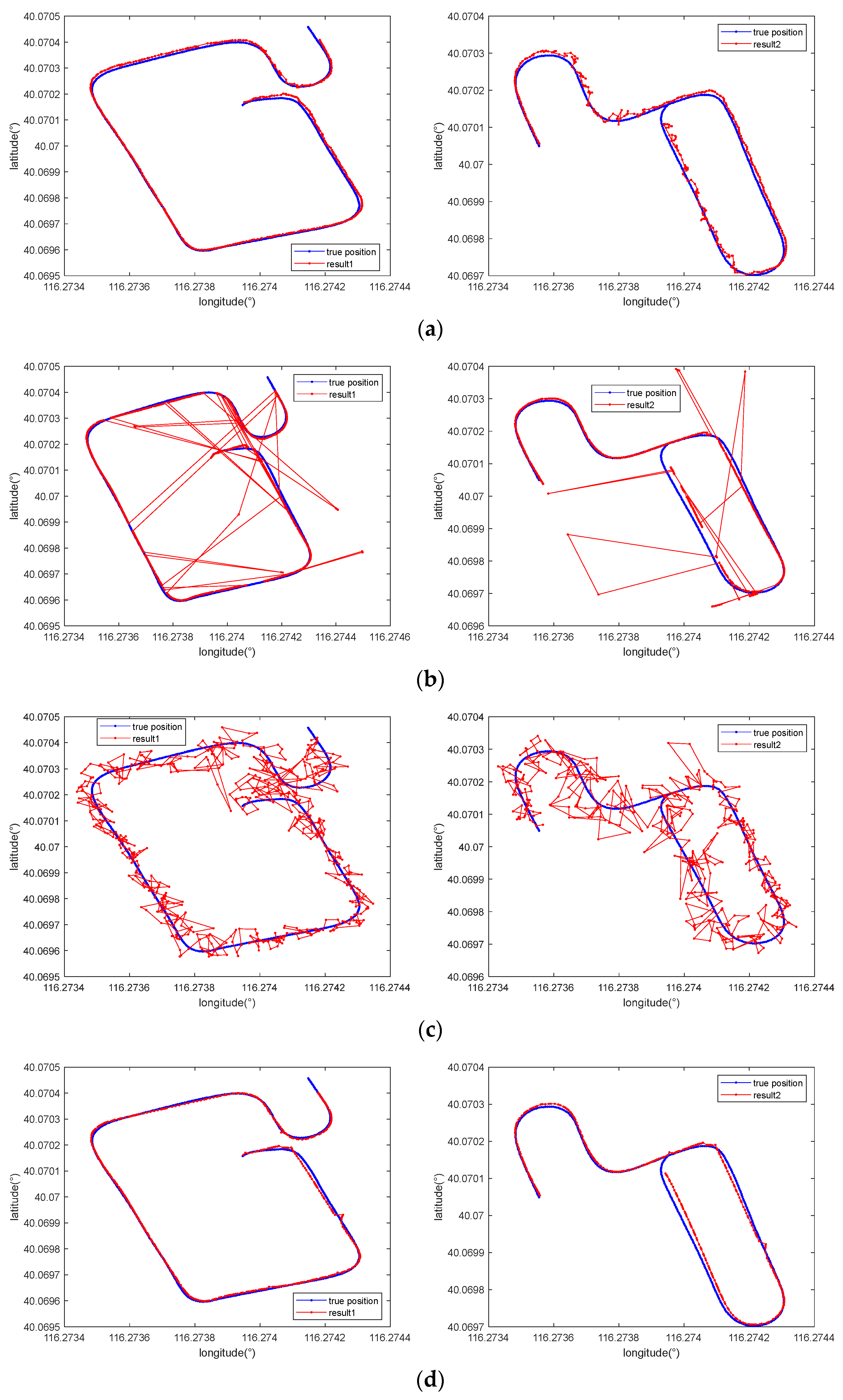
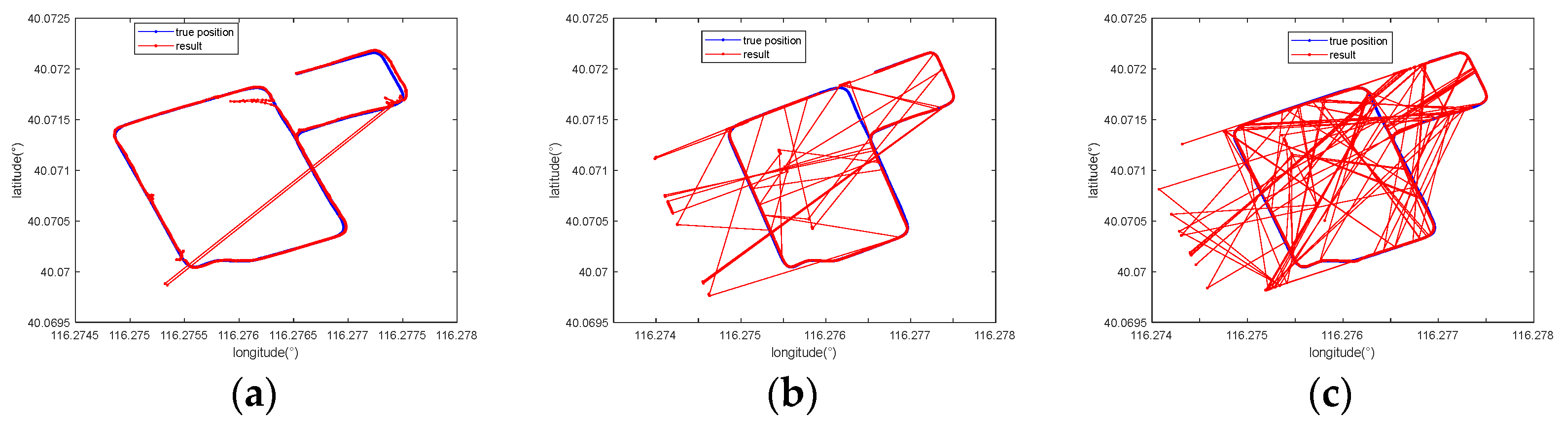
We selected 7-m-long sequences from two evaluation data to illustrate the effect of our method, whose positioning results are shown in Figure 11. The results suggest that in comparison with the traditional MAD-based matching method and the method in [12], whose matching results were chaotic and disorganized, the method in [27] and our method significantly reduced the degree of mismatching, producing results that closely fit the true positions.

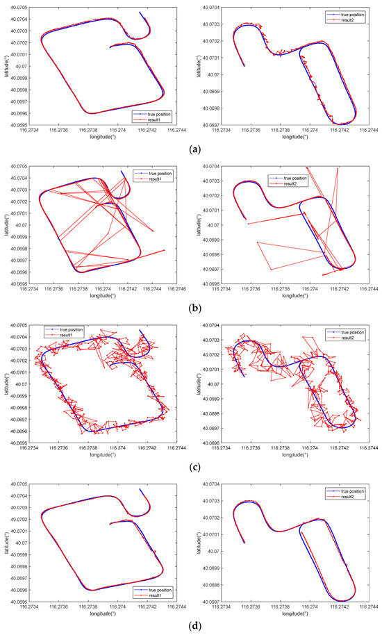
Figure 11. Comparison of the positioning results obtained with (a) the proposed method, (b) the traditional MAGCOM method using the MAD metric, (c) the method in [12], and (d) the method in [27] when using a 7-m-long sequence for various tracks.

Finally, we calculated the testing time of our method and compared it to that of other methods with a 7-m-long sequence. As shown in Table 4, the traditional method was superior to the learning-based methods in terms of time complexity, and our method took the longest calculation time due to the large size of the network. Considering that the speed of vehicles in the garage is usually less than 20 km/h, the average calculation time of 52.63 ms almost meets real-time positioning needs.

Table 4. The average testing time (ms) induced by different methods.

Methods
Proposed method	Traditional MAGCOM method using the MAD metric	Method in [12]	Method in [27]
52.63 ms	0.52 ms	27.03 ms	6.85 ms

4.3. Ablation Study

To further illustrate the importance of each module in the proposed method, we conducted ablation experiments in this section.

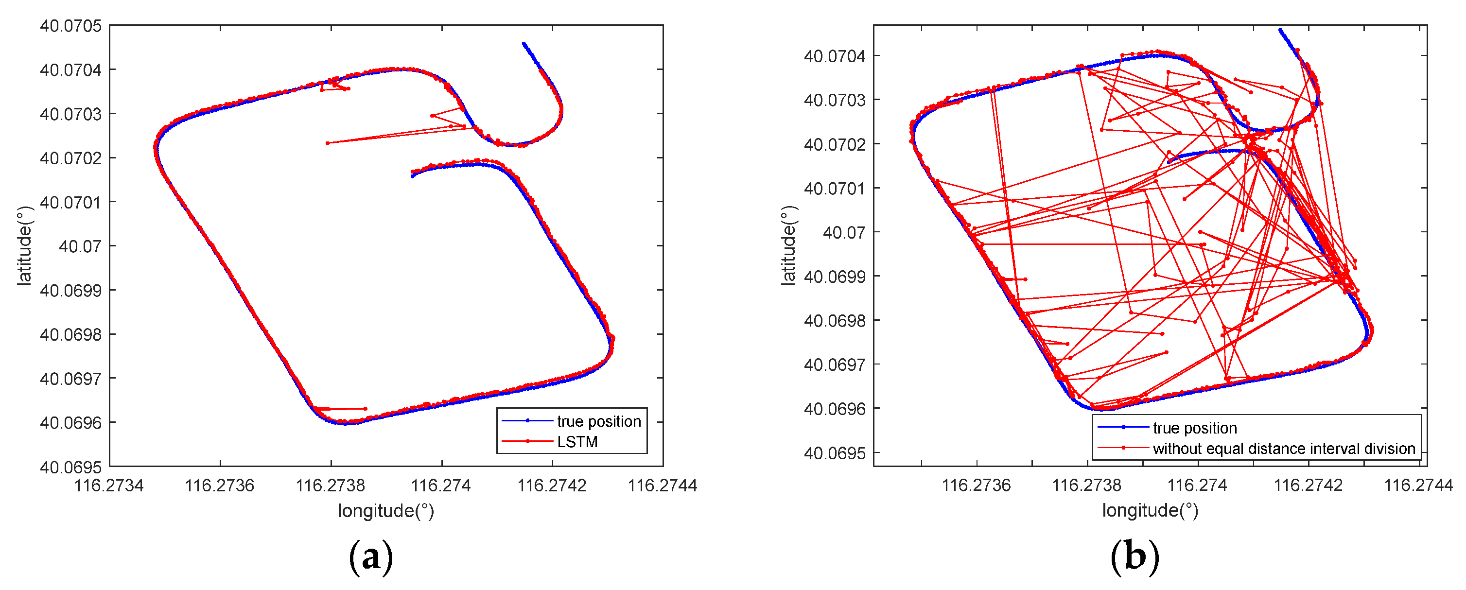
First, to verify the role of Transformer, it was replaced with an LSTM module [39] that has achieved success in magnetic localization tasks. The first and second columns in Table 5 demonstrate the maximum errors achieved with Transformer and LSTM, respectively, with a 7-m-long sequence as the input. It can be seen that their results were sometimes similar. However, for some tracks, the maximum errors of LSTM were larger than 10 m, which significantly influenced its positioning performance, such as that attained for tracks 1, 2, and 4. Figure 12a shows the positioning results yielded by LSTM for track 1. According to the comparison shown in the first plot of Figure 11a, our method yielded more accurate and more stable results.

Table 5. The maximum errors (m) induced by different methods.

Method	Sequence Length	Evaluation Data
		1	2	3	4	5	6	7	8
Proposed method	7 m	2.69	4.20	1.84	3.50	3.28	3.22	4.63	1.82
LSTM	7 m	22.89	11.82	1.45	12.02	3.59	1.70	8.55	1.62
Without the equal distance interval division module	≈7 m (2 s)	32.83	31.19	75.06	31.67	29.99	30.75	53.49	74.98

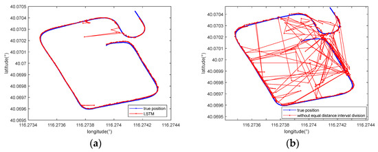
Figure 12. Comparison between the positioning results obtained with (a) LSTM and (b) the method removing the equal distance interval division module when using a 7-m-long sequence for track 1.

On the other hand, to indicate the effectiveness of the equal distance interval division strategy, it was removed before obtaining the positioning results. To conduct a fair comparison, the number of input points was set to 20 to ensure a sequence length of approximately 7 m when the average speed of the vehicle was 3.5 m/s and the magnetic data were sampled at 10 Hz. As shown in Figure 12b and the last column in Table 5, without the equal distance interval division module, the performance of the model drastically decreased.

In summary, the use of Transformer and the equal distance interval division strategy are both essential for our method.

4.4. Generalization Analysis

Many factors may affect the robustness of the positioning methods, including changes of the surroundings and the size of the positioning area. In this section, we conducted several additional experiments under different testing conditions to evaluate the influence of these factors on our method. The information concerning every validation dataset is shown in Table 6.

Table 6. Information concerning the three evaluation data.

Evaluation Data	Surroundings	The Size of Area
1	Full of cars	A small area as shown in Figure 10
2	Nearly no cars
3	/	A large area

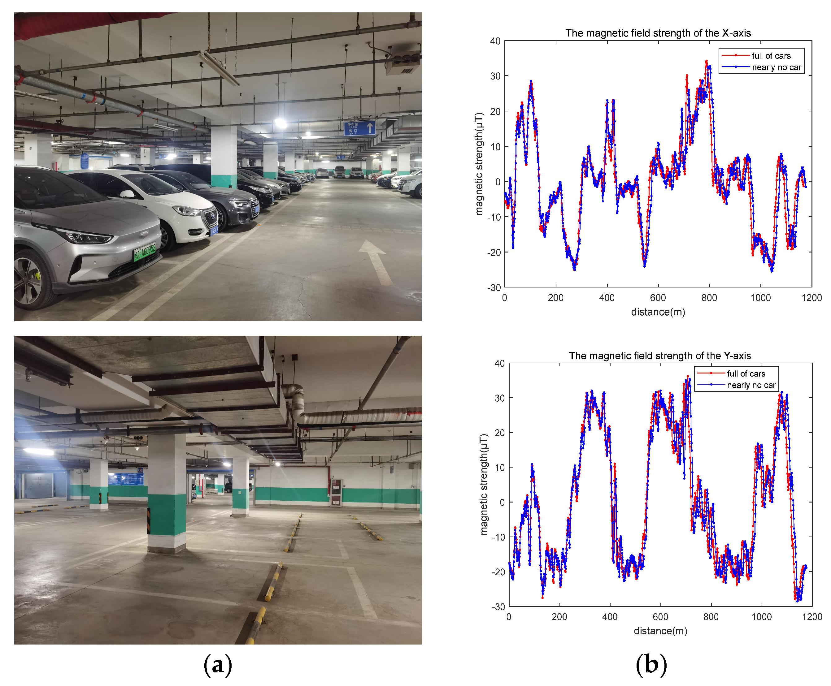
First, we estimated the impact of different surroundings. The validation data 1 were collected on a weekday morning, when the parking garage was full of cars, while the validation data 2 were collected on a weekend night, when almost no vehicles were in the parking garage, as shown in Figure 13a. The track is the same as the 7th evaluation data in Section 4.2.

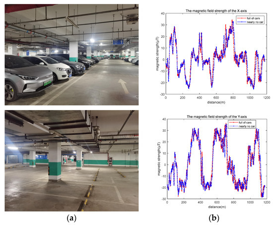
Figure 13. (a) Different surroundings; (b) measured magnetic fields in different surroundings.

The mean and maximum errors of our method with 7-m-long sequences are shown in Table 7. Compared to the results for the same track and sequences of the same length, the mean and maximum errors are very close to those in Table 2 and Table 3. In other words, the positioning results were almost unaffected by environmental changes.

Table 7. The mean and maximum errors (m) in different surroundings.

Method	Type of Error	Evaluation Data
		1	2
Proposed method	mean	1.31	1.51
	max	4.02	4.98

This may be attributed to two reasons. On the one hand, the data we used during the training process were collected in different surroundings, so the network is suitable for different surroundings. On the other hand, as seen from the plots in Figure 13b, although the measured magnetic fields are slightly different at the same position in different surroundings, the shapes of the magnetic field signal sequences are very similar for the same driving route, which has less impact on the sequence-based magnetic field positioning.

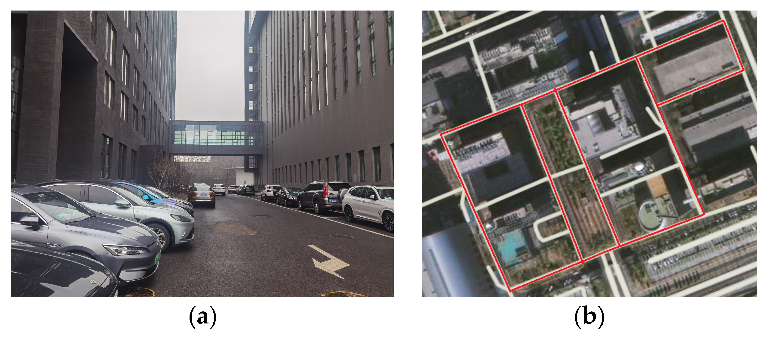
Second, we tested the ability of our method in a larger area. In validation data 3, the magnetic fields were collected in a large ground parking garage in urban canyon areas with dense buildings at the Beijing New Technology Base of the Chinese Academy of Sciences, which has an area of approximately 170 × 310 m², as shown in Figure 14a. The red lines in Figure 14b are the driving routes in this area.

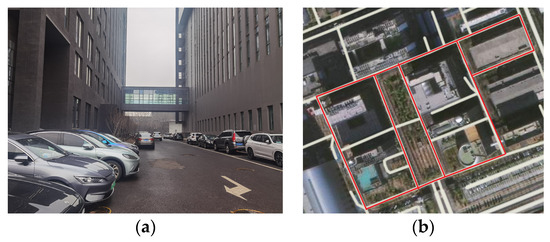
Figure 14. (a) A large ground parking garage in an urban canyon area with dense buildings; (b) driving routes.

The mean and maximum errors of our method for sequences of different lengths are shown in Table 8. Compared to a small area, a longer distance was needed to distinguish the shape of the magnetic field sequence at different locations in a larger area. In addition, we also compared our method with other methods shown in Section 4.2., except for the method in [12] because the network did not converge during the training phase. As shown in Table 8, the positioning errors and required sequence length were both less than those of the other two methods.

Table 8. The mean and maximum errors (m) induced by different methods in a larger area.

Method	Type of Error	Sequence Length
		35 m	40 m	45 m
Proposed method	mean	0.65	0.60	0.52
	max	84.68	4.76	4.39
Traditional MAGCOM method using the MAD metric	mean	16.61	1.40	0.74
	max	313.27	95.80	3.10
Method in [27]	mean	4.47	3.52	4.06
	max	97.39	100.65	88.49

Figure 15 represents the positioning results of three methods with 35-m-long sequences in a large area. Although the above methods all have incorrect positioning points, our method has the least number of errors.

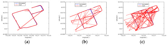
Figure 15. Comparison of the positioning results obtained with (a) the proposed method, (b) the traditional MAGCOM method using the MAD metric, and (c) the method in [27] using a 35-m-long sequence.

5. Conclusions and Future Work

This paper presents a magnetic localization method for vehicles in which a neural network based on Transformer is established to extract magnetic features and learn the relationships among points within a sequence. This process is performed after implementing equal distance interval division based on the given mileage. The experimental results illustrate the importance of each module in the proposed method, which achieves greatly improved magnetic positioning accuracy and reduces the required sequence length.

In the future, we plan to further develop this localization method in two ways. First, an adaptive sequence length should be developed according to the feature distribution of the magnetic field, as such a paradigm is more flexible than the use of a fixed sequence length. Second, considering that vehicles usually travel along existing paths, we expect to achieve a more accurate and reliable positioning performance by limiting the positioning results to paths.

References

- Shin, B.; Lee, J.; Yu, C.; Kyung, H.; Lee, T. Magnetic Field-Based Vehicle Positioning System in Long Tunnel Environment. Appl. Sci. 2021, 11, 11641. [Google Scholar] [CrossRef]
- Zhang, T.; Xu, X. A New Method of Seamless Land Navigation for GPS/INS Integrated System. Measurement 2012, 45, 691–701. [Google Scholar] [CrossRef]
- Paul, D.G.A. Principles of GNSS, Inertial, and Multi-Sensor Integrated Navigation Systems; Artech: London, UK, 2013. [Google Scholar]
- Sun, M.; Wang, Y.; Joseph, W.; Plets, D. Indoor Localization Using Mind Evolutionary Algorithm-Based Geomagnetic Positioning and Smartphone IMU Sensors. IEEE Sens. J. 2022, 22, 7130–7141. [Google Scholar] [CrossRef]
- El-Sheimy, N.; Youssef, A. Inertial Sensors Technologies for Navigation Applications: State of the Art and Future Trends. Satell. Navig. 2020, 1, 2. [Google Scholar] [CrossRef]
- Cheng, J.; Yang, L.; Li, Y.; Zhang, W. Seamless Outdoor/Indoor Navigation with WIFI/GPS Aided Low Cost Inertial Navigation System. Phys. Commun. 2014, 13, 31–43. [Google Scholar] [CrossRef]
- Abid, M.; Lefebvre, G. Improving Indoor Geomagnetic Field Fingerprinting Using Recurrence Plot-Based Convolutional Neural Networks. J. Locat. Based Serv. 2021, 15, 61–87. [Google Scholar] [CrossRef]
- Bitbrain. Available online: https://www.bitbrain.com/blog/indoor-positioning-system (accessed on 29 March 2024).
- Einsiedler, J.; Radusch, I.; Wolter, K. Vehicle Indoor Positioning: A Survey. In Proceedings of the 2017 14th Workshop on Positioning, Navigation and Communications (WPNC), Bremen, Germany, 25–26 October 2017; pp. 1–6. [Google Scholar]
- Li, B.; Gallagher, T.; Dempster, A.G.; Rizos, C. How Feasible Is the Use of Magnetic Field Alone for Indoor Positioning? In Proceedings of the 2012 International Conference on Indoor Positioning and Indoor Navigation (IPIN), Sydney, Australia, 13–15 November 2012; pp. 1–9. [Google Scholar]
- Lee, N.; Ahn, S.; Han, D. AMID: Accurate Magnetic Indoor Localization Using Deep Learning. Sensors 2018, 18, 1598. [Google Scholar] [CrossRef] [PubMed]
- Jang, H.J.; Shin, J.M.; Choi, L. Geomagnetic Field Based Indoor Localization Using Recurrent Neural Networks. In Proceedings of the GLOBECOM 2017—2017 IEEE Global Communications Conference, Singapore, 4–8 December 2017; pp. 1–6. [Google Scholar]
- Chen, J.; Ou, G.; Peng, A.; Zheng, L.; Shi, J. A Hybrid Dead Reckon System Based on 3-Dimensional Dynamic Time Warping. Electronics 2019, 8, 185. [Google Scholar] [CrossRef]
- Lu, Y.; Wei, D.; Ji, X.; Yuan, H. Review of Geomagnetic Positioning Method. Navig. Position. Timing 2022, 9, 118–130. [Google Scholar] [CrossRef]
- Wei, D.; Ji, X.; Li, W.; Yuan, H.; Xu, Y. Vehicle Localization Based on Odometry Assisted Magnetic Matching. In Proceedings of the 2017 International Conference on Indoor Positioning and Indoor Navigation (IPIN), Sapporo, Japan, 18–21 September 2017; pp. 1–6. [Google Scholar]
- Ji, X.; Wei, D.; Li, W.; Lu, Y.; Yuan, H. A GM/DR Integrated Navigation Scheme for Road Network Application. In Proceedings of the 2019 International Conference on Indoor Positioning and Indoor Navigation (IPIN), Pisa, Italy, 30 September 2019; pp. 117–124. [Google Scholar]
- Li, Y.; Zhuang, Y.; Lan, H.; Zhang, P.; Niu, X.; El-Sheimy, N. WiFi-Aided Magnetic Matching for Indoor Navigation with Consumer Portable Devices. Micromachines 2015, 6, 747–764. [Google Scholar] [CrossRef]
- Shu, Y.; Bo, C.; Shen, G.; Zhao, C.; Li, L.; Zhao, F. Magicol: Indoor Localization Using Pervasive Magnetic Field and Opportunistic WiFi Sensing. IEEE J. Select. Areas Commun. 2015, 33, 1443–1457. [Google Scholar] [CrossRef]
- Wu, Z.; Xu, Q.; Li, J.; Fu, C.; Xuan, Q.; Xiang, Y. Passive Indoor Localization Based on CSI and Naive Bayes Classification. IEEE Trans. Syst. Man Cybern. Syst. 2018, 48, 1566–1577. [Google Scholar] [CrossRef]
- Hoang, M.T.; Zhu, Y.; Yuen, B.; Reese, T.; Dong, X.; Lu, T.; Westendorp, R.; Xie, M. A Soft Range Limited K-Nearest Neighbors Algorithm for Indoor Localization Enhancement. IEEE Sens. J. 2018, 18, 10208–10216. [Google Scholar] [CrossRef]
- Lee, N.; Han, D. Magnetic Indoor Positioning System Using Deep Neural Network. In Proceedings of the 2017 International Conference on Indoor Positioning and Indoor Navigation (IPIN), Sapporo, Japan, 18–21 September 2017; pp. 1–8. [Google Scholar]
- Kim, D.; Bang, H.; Lee, J.C. Approach to Geomagnetic Matching for Navigation Based on a Convolutional Neural Network and Normalised Cross-correlation. IET Radar Sonar Navig. 2019, 13, 1323–1332. [Google Scholar] [CrossRef]
- Al-homayani, F.; Mahoor, M. Improved Indoor Geomagnetic Field Fingerprinting for Smartwatch Localization Using Deep Learning. In Proceedings of the 2018 International Conference on Indoor Positioning and Indoor Navigation (IPIN), Nantes, France, 24–27 September 2018; pp. 1–8. [Google Scholar]
- Abid, M.; Compagnon, P.; Lefebvre, G. Improved CNN-Based Magnetic Indoor Positioning System Using Attention Mechanism. In Proceedings of the 2021 International Conference on Indoor Positioning and Indoor Navigation (IPIN), Lloret de Mar, Spain, 29 November 2021; pp. 1–8. [Google Scholar]
- Bae, H.J.; Choi, L. Large-Scale Indoor Positioning Using Geomagnetic Field with Deep Neural Networks. In Proceedings of the ICC 2019—2019 IEEE International Conference on Communications (ICC), Shanghai, China, 20–24 May 2019; pp. 1–6. [Google Scholar]
- Wang, X.; Yu, Z.; Mao, S. DeepML: Deep LSTM for Indoor Localization with Smartphone Magnetic and Light Sensors. In Proceedings of the 2018 IEEE International Conference on Communications (ICC), Kansas City, MO, USA, 20–24 May 2018; pp. 1–6. [Google Scholar]
- Wang, L.; Luo, H.; Wang, Q.; Shao, W.; Zhao, F. A Hierarchical LSTM-Based Indoor Geomagnetic Localization Algorithm. IEEE Sens. J. 2022, 22, 1227–1237. [Google Scholar] [CrossRef]
- Wang, Q.; Wang, L.; Fu, M.; Wang, J.; Sun, L.; Huang, R.; Li, X.; Jiang, Z.; Luo, H. Multi-Scale Transformer and Attention Mechanism for Magnetic Spatiotemporal Sequence Localization. IEEE Internet Things J. 2024, 1. [Google Scholar] [CrossRef]
- Njima, W.; Chafii, M.; Shubair, R.M. GAN Based Data Augmentation for Indoor Localization Using Labeled and Unlabeled Data. In Proceedings of the 2021 International Balkan Conference on Communications and Networking (BalkanCom), Novi Sad, Serbia, 20 September 2021; pp. 36–39. [Google Scholar]
- Vaswani, A.; Shazeer, N.; Parmar, N.; Uszkoreit, J.; Jones, L.; Gomez, A.N.; Kaiser, L.; Polosukhin, I. Attention Is All You Need. In Proceedings of the 31st Conference on Neural Information Processing Systems (NIPS 2017), Long Beach, CA, USA, 4–9 December 2017. [Google Scholar]
- Ba, J.L.; Kiros, J.R.; Hinton, G.E. Layer Normalization. arXiv 2016, arXiv:1607.06450. [Google Scholar]
- Torres-Sospedra, J.; Rambla, D.; Montoliu, R.; Belmonte, O.; Huerta, J. UJIIndoorLoc-Mag: A New Database for Magnetic Field-Based Localization Problems. In Proceedings of the 2015 International Conference on Indoor Positioning and Indoor Navigation (IPIN), Banff, AB, Canada, 13–16 October 2015; pp. 1–10. [Google Scholar]
- Hanley, D.; Faustino, A.B.; Zelman, S.D.; Degenhardt, D.A.; Bretl, T. MagPIE: A dataset for indoor positioning with magnetic anomalies. In Proceedings of the 2017 International Conference on Indoor Positioning and Indoor Navigation (IPIN), Sapporo, Japan, 18–21 September 2017; pp. 1–8. [Google Scholar] [CrossRef]
- Barsocchi, P.; Crivello, A.; La Rosa, D.; Palumbo, F. A Multisource and Multivariate Dataset for Indoor Localization Methods Based on WLAN and Geo-Magnetic Field Fingerprinting. In Proceedings of the 2016 International Conference on Indoor Positioning and Indoor Navigation (IPIN), Alcala de Henares, Spain, 4–7 October 2016; pp. 1–8. [Google Scholar]
- Tóth, Z.; Tamás, J. Miskolc IIS hybrid IPS: Dataset for hybrid indoor positioning. In Proceedings of the 2016 26th International Conference Radioelektronika (RADIOELEKTRONIKA), Kosice, Slovakia, 19–20 April 2016; pp. 408–412. [Google Scholar] [CrossRef]
- Ashraf, I.; Din, S.; Ali, M.U.; Hur, S.; Zikria, Y.B.; Park, Y. MagWi: Benchmark Dataset for Long Term Magnetic Field and Wi-Fi Data Involving Heterogeneous Smartphones, Multiple Orientations, Spatial Diversity and Multi-Floor Buildings. IEEE Access 2021, 9, 77976–77996. [Google Scholar] [CrossRef]
- IMU-ISA-100C Product Sheet. Available online: https://www.amtechs.co.jp/product/IMU-ISA-100C%20Product%20Sheet_v7.pdf (accessed on 9 February 2024).
- GovCDO. Available online: https://www.digitalelite.cn/h-pd-1259.html (accessed on 29 March 2024).
- Greff, K.; Srivastava, R.K.; Koutník, J.; Steunebrink, B.R.; Schmidhuber, J. LSTM: A Search Space Odyssey. IEEE Trans. Neural Netw. Learn. Syst. 2017, 28, 2222–2232. [Google Scholar] [CrossRef] [PubMed]
Disclaimer/Publisher’s Note: The statements, opinions and data contained in all publications are solely those of the individual author(s) and contributor(s) and not of MDPI and/or the editor(s). MDPI and/or the editor(s) disclaim responsibility for any injury to people or property resulting from any ideas, methods, instructions or products referred to in the content. |
© 2024 by the authors. Licensee MDPI, Basel, Switzerland. This article is an open access article distributed under the terms and conditions of the Creative Commons Attribution (CC BY) license (https://creativecommons.org/licenses/by/4.0/).