1. Introduction
The depth of frost penetration holds considerable significance in the design of diverse infrastructure elements, spanning from building foundations to transportation networks, including pavements, retaining structures, and bridge foundations. Soil freezing can instigate frost heave and resultant pressure, posing significant stability concerns. This heave has the potential to induce notable vertical and lateral stresses and movements, leading to ground surface uplift caused by water freezing within soil layers. Consequently, foundations may be lifted, or substantial additional stresses may be imposed on exposed retaining structures. Furthermore, frost heave typically precedes thaw consolidation and settlement, leading to fluctuating vertical movements in spread footings positioned on soils subjected to freeze–thaw cycles. Such movements can cause extensive damage to various civil engineering structures, such as pavements and utility lines. To counteract the adverse effects of frost, foundations are commonly constructed below the frost line.
The last official standard of Romania related to frost penetration was issued in 1977, “Maximum freezing depths”, which zoned Romania’s territory by freezing depth, according to STAS 6054/77 [
1]. Now, this paper compares the methods widely used for soil freezing determination, and the results are compared with the actual soil freezing map of Romania.
The selected methods for estimating the winter climatic design parameters are used by different international organizations and countries: the NOAA, the USACE, Eurocodes/the International Standard Organization, Poland, and Russia.
In this study, we determine frost- and heave-related parameters using extreme value distributions, specifically the Gumbel distribution. Extreme value distributions represent the limiting distributions for either the minimum or maximum values within a significantly large set of random observations originating from the same arbitrary distribution. These distributions are particularly relevant when analyzing natural hazards such as snow, wind, temperature, floods, and similar phenomena. All the frost/heave design-related parameters were calculated for all 111 meteorological stations in Romania for the 1900–2020, 1950–2020, 1950–1990, and 1990–2020 periods. By taking the locations (geographical coordinates and altitudes) of the 3186 administrative–territorial units in Romania, the average temperature of the coldest quarter for all administrative units in Romania from the ECMWF COPERNICUS REPORT (global bioclimatic indicators from 1979 to 2018 derived from reanalysis), and the yearly average temperatures (Official Gazette of Romania), models were calibrated using the simple Kriging geostatistical method.
2. Winter Severity Parameters
The present study is based on the minimum and maximum daily air temperatures measured at the meteorological stations at 2 m above the surface.
Other databases used in the analysis were as follows:
The Copernicus Climate Change Service (ECMWF COPERNICUS REPORT, global bioclimatic indicators from 1979 to 2018 derived from reanalysis) [
2];
Geographical coordinates and altitudes for the 3186 administrative–territorial units, retrieved from Global Multi-Resolution Terrain Elevation Data 2010 (GMTED2010), [
3];
The Ensemble Version of the E-OBS Temperature and Precipitation Datasets [
4];
WorldClim version 2.1 climate data for 1970–2000;
Monthly average values and annual averages for 111 cities published in the Official Gazette of Romania;
Statistical indicators of the maximum negative and maximum positive annual temperatures for 128 meteorological stations.
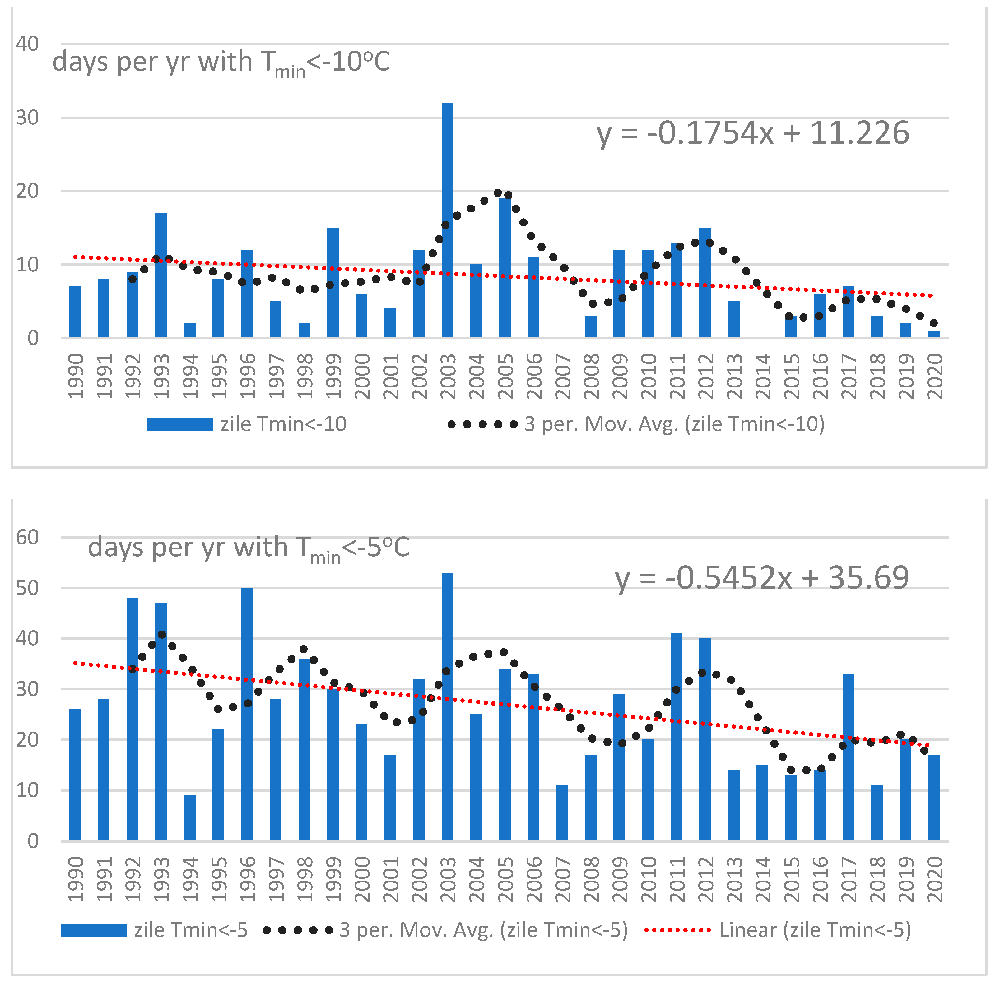
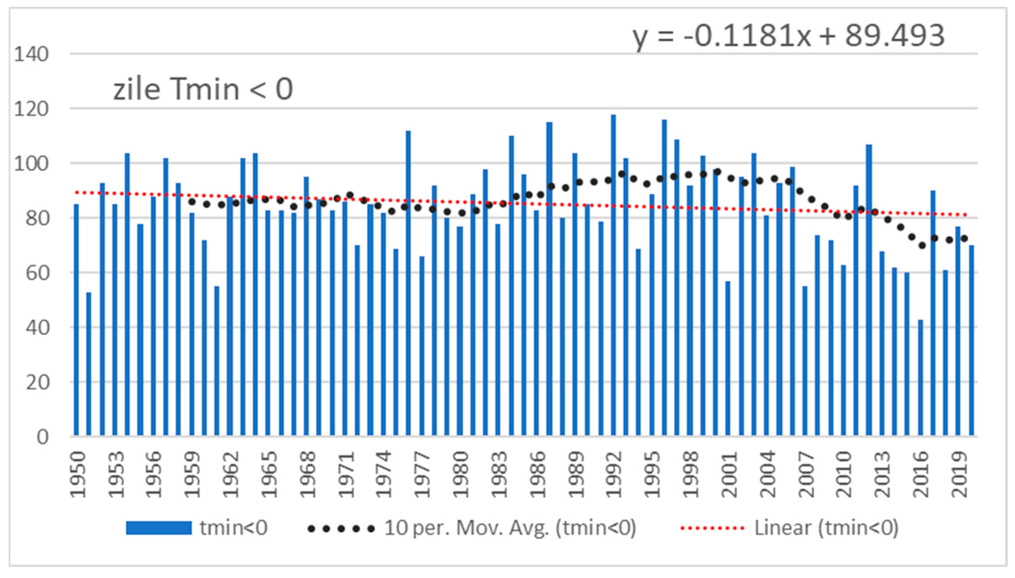
Due to recent climate instabilities, interest in the investigation of extreme weather and climate events has been increasing during the last few decades. The availability of information for the last 120 years made it possible to investigate the parameters of winter severity (Days with Tmin < −5 °C, Days with Tmin < −10 °C, Days with Tmax < 0 °C, Days with Tmax < −5 °C, Days with Tavg < 0 °C), taking into consideration the different time intervals of the catalogues of daily temperatures.
Figure 1 presents the trends of the number of days per year with minimum temperatures of less than −10 °C and −5 °C during the 1990–2020 period.
In
Table 1, we present statistical indicators of other parameters used to evaluate the winter severity. From the four selected time intervals, we can identify the differences between the maximum recorded days per year in the period 1990–2020 and the other time intervals considered in the analysis.
Another indicator of the winter severity is the length of the frost-free season (LFFS). The time of the occurrence of the last spring frost (LSF) and the first fall frost (FFF) determine the length of frost-free season (LFFS), which significantly impacts various aspects of human activity. In the last 20 years, at the Arad station, there has been an increase in the LFFS season in comparison with the period 1980–2000,
Figure 2.
The numbers presented in the
Table 1 indicate a general decrease in the average number of days with extreme cold temperatures (e.g., Tmin < −5 °C, Tmin < −10 °C, Tmax < 0 °C, Tmax < −5 °C, Tavg < 0 °C) as we move from earlier periods (1900–2020, 1950–2020, 1950–1990) to the most recent period (1990–2020).
This trend is particularly pronounced when comparing the 1990–2020 period to earlier periods. These trends suggest a gradual shift towards warmer temperatures at the Arad station area over the investigated periods, which could be indicative of broader climate change trends. Furthermore, it is important to note that these conclusions are based solely on the provided statistical parameters (i.e., the trendline equations presented in
Figure 1 and
Figure 2) and do not take into account other potential factors influencing temperature trends in the region.
3. Frost Depth Prediction
Frost depth is a function of the material type, soil thermal properties, soil water content, and climatic conditions such as temperature, wind speed, precipitation, and solar radiation, whether those factors are acting individually or as a whole.
The depth to which the ground freezes depends on the following factors: the duration and intensity of winter frosts, soil moisture, the presence and type of vegetation, and the thickness of snow cover. The soil freezing regime is also closely linked to local relief and microclimate features, which cause considerable variation within small areas.
In the case of forests, the frost depth is much lower than in open fields because of the protective role of vegetation and the stability of the snow cover in winter. The thicker the snow cover, the less frost penetrates the soil; the moist soils freeze less than dry soils because the latent heat from freezing water slows the spread of frost to lower depths. In sandy soils, the depth of frost is greater than in clay soils, which have better heat conductivity, and the marshlands and marshy soils freeze the least.
Existing frost depth prediction models can be classified into numerical, analytical, semi-empirical, and empirical models. Some models require as inputs various thermal and hydraulic properties of soil and different meteorological data [
5].
3.1. USA Standards/Regulations
There are several frost depth prediction models that have been developed and implemented by the US authorities. Some of these models are empirical in nature, while others are semi-empirical.
The reference methodology developed by the NOAA (National Oceanic and Atmospheric Administration) is based on the AFI calculation at each weather station. Using the NOAA’s National Climatic Data Center (NCDC), Billotta et al. 2015 [
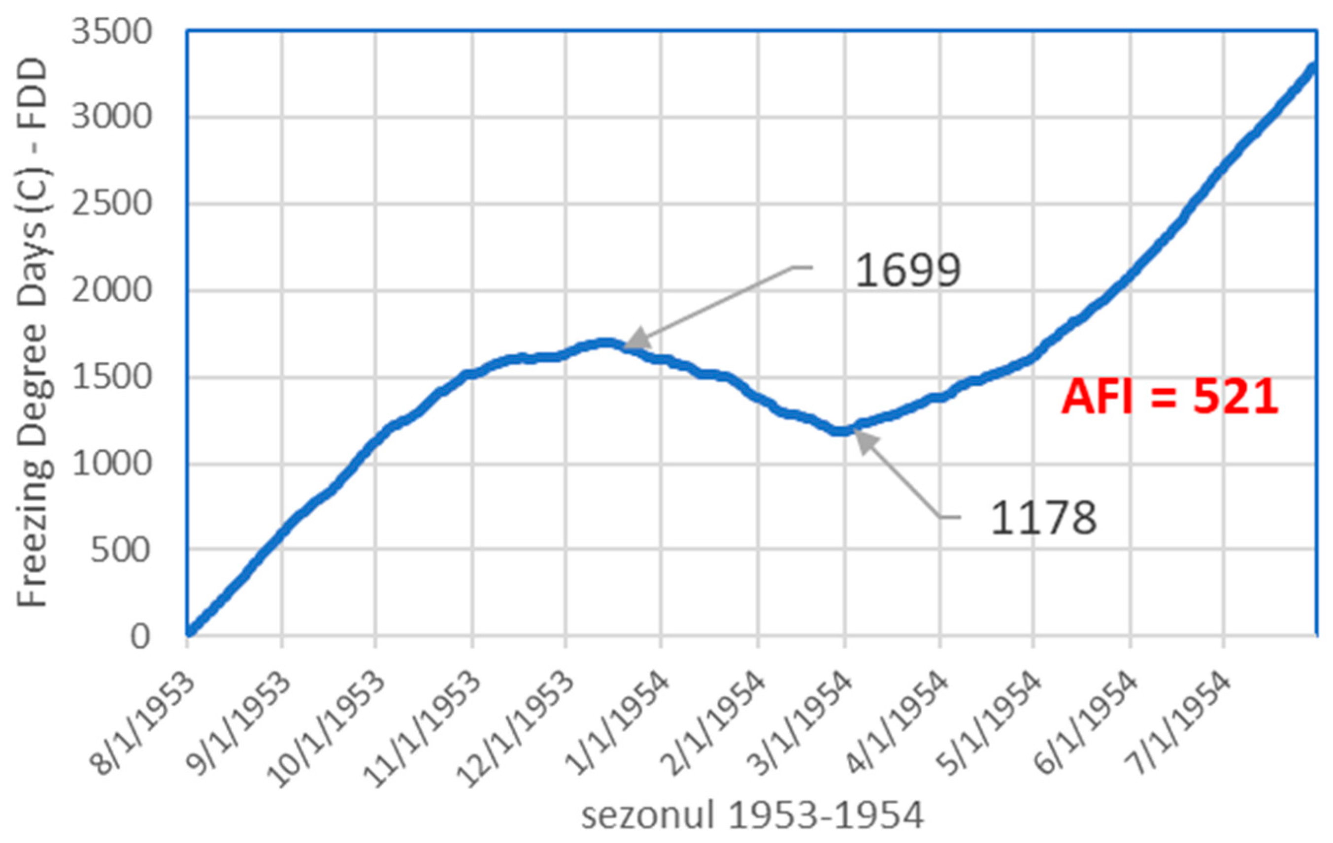
6] used the complete dataset of daily maximum and minimum temperatures that were utilized to calculate the NOAA’s 1981–2010 freezing degree days (FDDs) and the corresponding AFI values. The air-freezing index (AFI) is a common metric for determining the freezing severity of the winter season and estimating frost depth. AFI values represent the seasonal magnitude and duration of below-freezing air temperature. Departures from the daily mean temperature above or below 0 °C are accumulated over each August–July cold season are accumulated and can be plotted on a seasonal time curve. The difference between the highest and lowest extrema points on this seasonal curve is defined as the seasonal AFI value. For example, in
Figure 3, the most extreme AFI value for the Arad station over the 1900–2020 period occurred during the 1953/54 season, with an AFI value of 521 FDDs.
AFI is converted to frost depth using the Brown (1964) [
5] Formula (1).
where d
frost is the depth of frost for a bare ground surface (m) and AFI
100 is the 100-year return AFI (°C).
The AFI
100 is computed using generalized extreme value distribution analysis. In this study, we calculate all the parameters, with
xp corresponding to the return periods determined via the Gumbel distribution for maxima [
7].
The Gumbel distribution for maxima is defined by its cumulative distribution function, CDF:
where
u and
α are the parameters of the distribution.
and μ
x and σx are the mean and the standard deviation of the distribution.
The fractile
xp that is defined as the value of the random variable X with p non-exceedance probability (
P(
X ≤ xp) =
p) is computed as follows:
The values of
kpG for different non-exceedance probabilities are given in
Table 2.
Table 3 presents the statistical parameters (mean, standard deviation, and maximum recorded values) for the measured AFI and the corresponding return periods values for the Arad station. The depth of frost (in cm) is also presented for the four periods of time investigated.
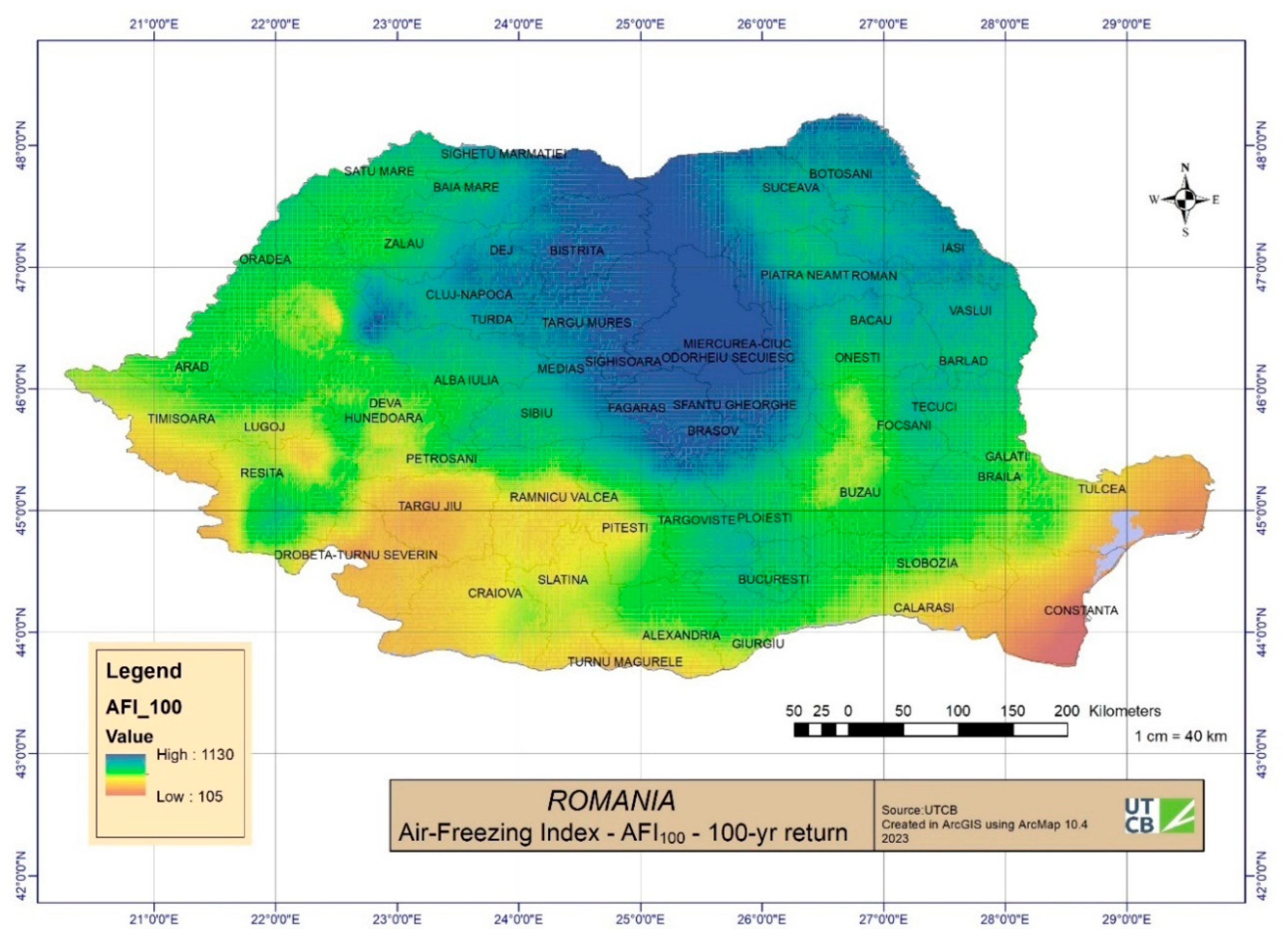
The 100-year return AFI values were calculated for all 111 meteorological stations in Romania for the 1950–2020 period. Based on the simple kriging geostatistical method,
Figure 4 presents the AFI
100 map of Romania. The statistical model takes into consideration the yearly average temperatures and the location and average temperature of the coldest quarter for all administrative units of Romania.
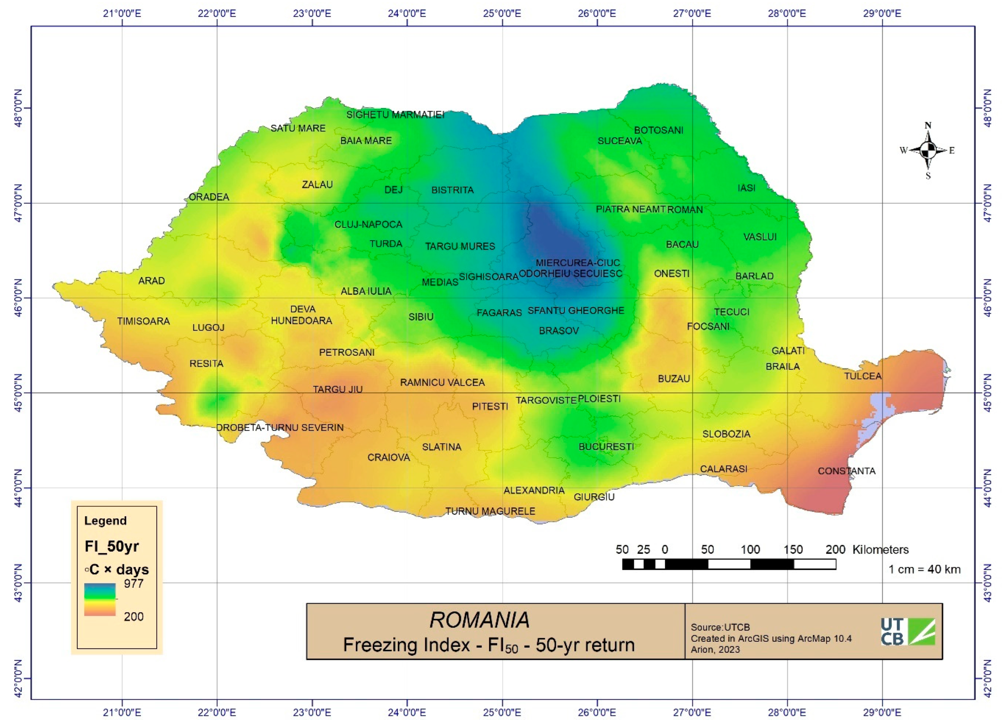
The reference methodology to calculate frost depth (cm) developed by the U.S. Corps of Engineers (Yoder, 1975) [
8] requires only the freezing index (FI) or the cumulative freezing degree day (CFDD), Equation (4). The freezing index is a measure of the combined duration and magnitude of below-freezing temperatures occurring during a specific freezing season and calculated via the summation in Celsius-degrees-hour (or below-freezing temperatures and subtracting from that the total number of Celsius-degree-hours (or days) above 0 °C over the same period).
The freezing index (FI) is based on the mean daily temperature. Many engineering calculations [
9], including, among other factors, the frost penetration depth, are based on the FI. Equation (4) does not separate sandy from clayey soils.
where d
frost, = frost depth (cm) and FI = cumulative freezing degree day (°C × day).
Based on the simple kriging geostatistical method,
Figure 5 presents the FI
50 map of Romania.
Table 4 presents the statistically measured FI, the corresponding return period values, and the depth of frost (in cm) for the Arad station.
3.2. ISO and European/UE Standards/Regulations
The methodology EN ISO 13793:2001 (thermal performance of buildings—thermal design of foundations to avoid frost heave) [
10] for frost depth prediction is based on the variation in air temperature during winter, which can be represented by the freezing index and Josef Stefan’s method (Stefan’s equation is one of the first known theoretical formulas to calculate frost penetration), as shown in Equation (5). The recommended values of the parameters from Equation (5) are for the worst-case scenario (bare ground surface over granular soils).
where:
Fd is the design freezing index, in K × h;
λf is the thermal conductivity of frozen soil, in W/(m × K)—2.5 W/(m × K);
L is the latent heat of freezing of water in the soil per volume of soil, in J/m3—150 × 106 J/m3;
C is the heat capacity of unfrozen soil per volume, in J/(m3 × K)—3 × 10⁶ J/(m3 × K) and
is the annual average external air temperature, in °C;
The design freezing index Fd is 24 times the FI, which is cumulative freezing degree day (°C × day).
For permanent structures, F100 or F50 must be used.
For the design of buildings/roads that can tolerate some movement, as well as for non-permanent buildings/structures, a lower freezing index (e.g., F20, F10, F5) may be used.
Table 5 presents the F
d (°C × h) values and the calculated frost depth, H
0 (m), for the Arad station. The values of
H0X are calculated with the same recommended values as the parameters of Equation (5), except of λ
f, which is set to the specific value of 1.5 W/(m × K) attributed to clayed soils.
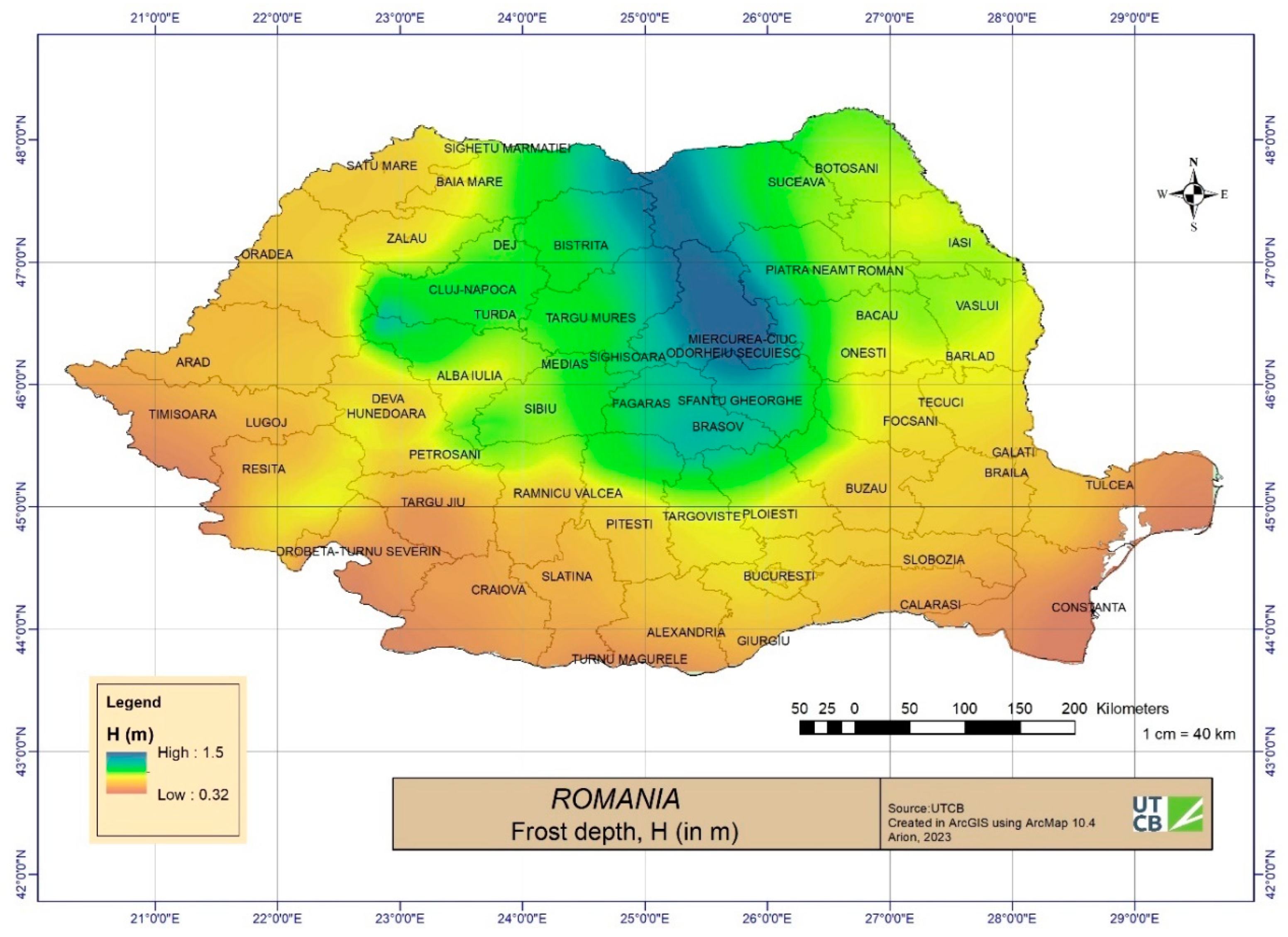
3.3. Russian and Polish Standards/Regulations
In Russia, according to paragraph 2.124 (2.27) of the manual for the design of the foundations of buildings and structures (Russian construction standard SNiP 2.02.01-83) and SNiP 2.01.01-84 Climatology and Geophysics, the frost depth, H (in m), is calculated very simply using Equation (6):
where:
M is the sum of the absolute values of the average monthly negative temperatures for the winter (only negative values are summarized);
K is coefficient equal to 0.23 for clays and silts, 0.28 for sandy clays and fine-grained sands, 0.30 for coarse-grained sands, and 0.34 for gravels.
For example, according to SNIP, a frost depth of 1.4 m is set for the Moscow region for severe meteorological conditions, for a high groundwater level, in the absence of snowmelt, and in severe frost conditions, although according to studies, the frost depth in the Moscow region varies from 60 cm to 180 cm.
Since 1955, the maps of the soil freezing depths have been given in the Polish Standards [
11]. The values of frost depth, H, are calculated in centimeters according to the formula given in Soviet recommendations, as shown in Snip:
where
M and
K are the same as the ones from the Russian norms. In both norms, there are no references to the return periods of the values.
The depth of frost (in m) for the Arad station calculated for the coarse-type ground by using the Russian norm is 0.34 m, and it is calculated as 0.57 m by using the Polish norm. The application of Equation (7) for Romanian territory in the worst-case scenario (k = 0.34—gravely soils) is presented in
Figure 6.
The “Zoning of Romania’s territory by freezing depth”, STAS 6054/77, specifies for the Arad station a 70–80 cm frost depth. In comparison, in
Table 6, there are values of depths of frost with different mean recurrence intervals (MRI, 100, 50, 20, and 10 years), calculated for different periods and via different methodologies.
4. Evaluation of Frost Heave/Freeze–Thaw Cycle (FTC)
The freeze–thaw cycle (FTC) is defined as a cycle in which the temperature fluctuates both above and below 0 °C [
12]. The minimum temperature of 0 °C is used as the threshold for freezing to increase the likelihood that water froze at the surface.
The determination of the number of days with FTC occurrence potential, for each year, for a different investigated period, was calculated in accordance with the two measured parameters: daily maximum temperature (T
max) and daily minimum temperature (T
min) [
13].
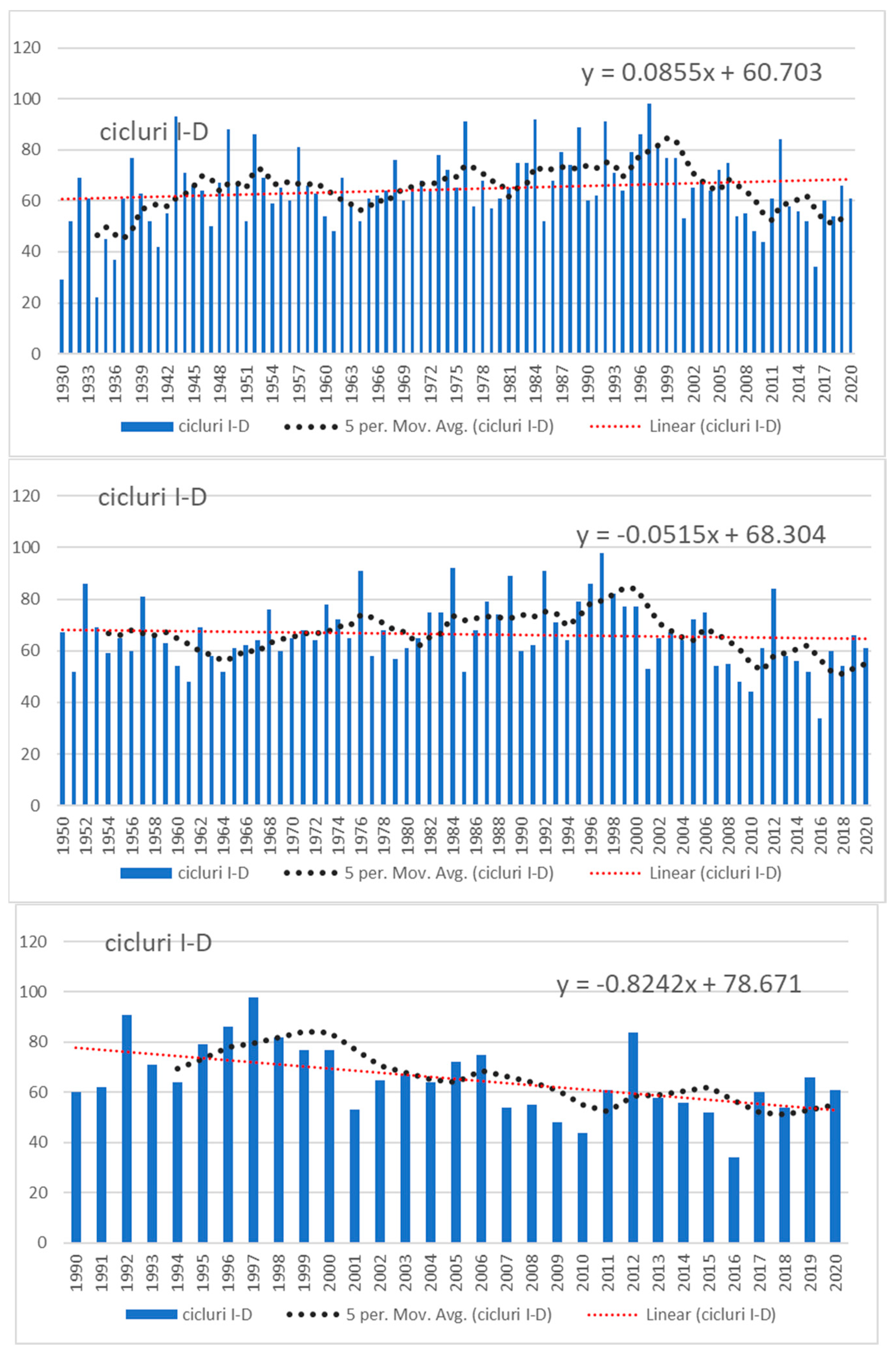
Figure 7 highlights the trend of the number of FTCs during the three investigated periods.
The FTC10, FTC50, and FTC100 (FTCs with different return periods: 10 years, 50 years, and 100 years) for available meteorological stations are computed using generalized extreme value distribution analysis.
Table 7 shows the statistical parameters (mean, standard deviation, and maximum recorded) of the yearly FTCs during different periods for the Arad Station. Also in
Table 7, the FTC values are for 10-year, 50-year, and 100-year return periods.
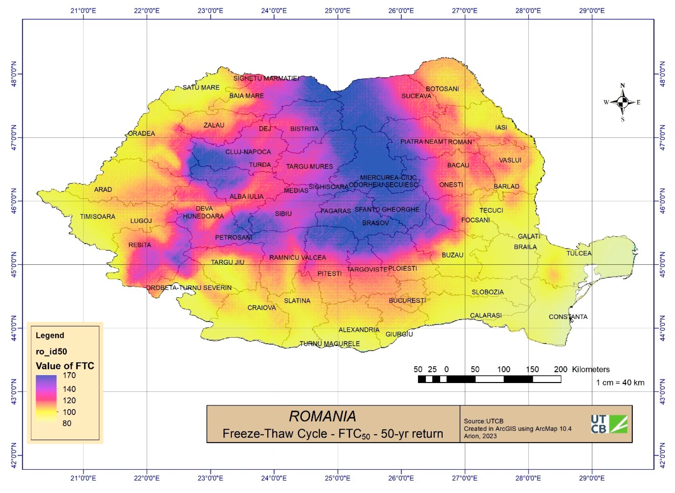
The 50-year return FTC values were calculated using the Gumbel value distribution for all 111 meteorological stations in Romania for the 1950–2020 period. Based on the simple kriging geostatistical method,
Figure 8 presents the FTC
50 map of Romania.
Sulina and Miercurea Ciuc stand out as the most extreme locations when considering winter parameters. The frost-free period, denoted by the average values (LFFS), ranges from 319 days in Sulina along the Black Sea to 203 days in Miercurea Ciuc, reflecting the negative relief forms of the Inter-Carpathian Depression in the central part of Romania. Calculations based on extreme frost dates (50-year return period) indicate a reduction in the frost-free period to 268 days in Sulina and 138 days in Miercurea Ciuc.
5. Conclusions
Evaluating soil frost depth is difficult because direct measurements of frost depth are not widely available and those that are available do not date back very far. As frost depth is closely linked to air temperatures, an index that measures how often, and by how much, air temperatures remain below freezing through the winter can serve as a useful proxy measurement for frost depth. The isolines/maps were smoothed using the kriging method. Some caution should be used with spatially interpolated results. The most recognized flaw in this method is that interpolation assumes that the spatial area is homogeneous across the surface.
The statistical models were calibrated by taking into consideration the yearly average temperatures (Official Gazette of Romania by ANM), the location (geographical coordinates and altitudes for 3186 administrative-territorial units retrieved from the Global Multi-Resolution Terrain Elevation Data 2010), and the average temperature of the coldest quarter for all administrative units of Romania (ECMWF COPERNICUS REPORT, global bioclimatic indicators from 1979 to 2018 derived from reanalysis).
An accurate estimate of maximum soil frost depth allows for reduced construction costs and proper preparations for future climate conditions. Soil frost depth also has important implications for hydrology, agriculture, and even burials.
Due to the influence of both the duration and severity of sub-zero temperatures, the warming trends observed in the past three decades are likely to be modifying the freezing patterns of soil and contributing to an increase in the freeze–thaw cycle (FTC). The increase in the FTC can lead to significant structural damage to buildings, roads, and other structures. FTCs have also important implications for hydrology and agriculture.
In the climatic conditions of Romania, there is an inter-annual very high variability in the dates of the disappearance of the last spring ground frosts and the dates of the occurrence of the first autumn ground frosts, as well as in the number of days with the phenomenon and the duration of frost-free period. The values from the maps represent the worst case scenario expected in each area.
We retrieved the available data from the National Oceanic and Atmospheric Administration (
https://www.noaa.gov/, accessed on 5 May 2022) and the National Meteorological Agency (a governmental organization organized under the authority of Romanian Environment Ministry).
We acknowledge the E-OBS dataset from the EU-FP6 project UERRA (
https://www.uerra.eu, accessed on 5 May 2022) and the Copernicus Climate Change Service, as well as the data provides by the ECA&D project (
https://www.ecad.eu, accessed on 5 May 2022).


