Abstract
In regions with severe cold and high latitudes, concrete structures are susceptible to cracking and displacement due to uneven temperature stress, which directly impacts their normal utilization. Therefore, to investigate the temperature distribution characteristics of concrete box girders under the combined influence of low temperatures and cold waves, a temperature test was conducted on a model of concrete box girders in Xinjiang Province, China. Based on the measured data, the distribution pattern of the most unfavorable negative temperature differential observed in high-latitude regions was determined. Long-term numerical simulation and extreme value analysis were performed using historical meteorological data, revealing that the vertical negative temperature gradient in the concrete box girder structures follows a composite exponential distribution. The temperature differential at the top complies with Chinese code requirements, while at the bottom, it aligns more closely with British standard BS5400. Statistical analysis of historical meteorological data predicts that the 50-year temperature differential will result in a drop amplitude of 26.42 °C, which is 1.44 times higher than measured values obtained from experiments. The proposed negative temperature gradient pattern for concrete box girders presented in this study can encompass general design codes and provide guidance for designing concrete bridges in severe cold areas.
1. Introduction
The internal temperature distribution of concrete box girders is nonlinear and influenced by factors such as air temperature, solar radiation, and wind speed. Fluctuations in average temperature and vertical and lateral temperature gradients exacerbate the cracking and excessive displacement of the girder, thereby affecting its normal use [1,2]. The effects of regional variations in temperature on concrete structures are evident due to differences in environmental climates, particularly in high-latitude areas. Severe winter weather conditions pose a threat to the safety of concrete structures by inducing significant temperature stresses [3]. Therefore, conducting research on the temperature effects of concrete structures in high-latitude areas is imperative for providing valuable insights into construction and operation practices within such environments.
The Altay region of Xinjiang is in a high-latitude area, and extensive research has been conducted by various scholars on the climate change associated with severe winter weather in this region. Fan et al. [4] have revealed the spatial–temporal variations in severe winter weather, while Bai et al. [5] focused on the variation characteristics of cold wave activity, providing insights into the impact of climate change on cold wave mechanisms. Given the increasing frequency and intensity of extreme weather and climate events globally [6], climate change has garnered significant attention from scholars worldwide. DelSole and Quesada [7,8] have investigated the extreme cold climate variables in North America and Europe based on observations as well as general circulation models, whereas Messori and Faranda [9] have identified interactions between large-scale atmospheric circulation in North America and simultaneous outbreaks of cold spells in Europe. Due to the distinct geographical conditions between Europe, the United States, and Xinjiang, it is crucial to recognize that the process governing cold wave weather may differ across these regions. Consequently, studying cold wave weather phenomena in high-latitude regions remains an important focus for current and future research endeavors.
The temperature distribution of concrete box girders and its influencing factors under cold wave conditions have been a prominent research focus in the field of engineering. Previous studies have examined the impact of key factors, such as solar radiation and air temperature changes, on the structural behavior of concrete box girders [10,11,12]. They have also proposed models to predict temperature gradients under ambient thermal loads. For instance, Lee et al. [13] investigated temperature differentials and thermal deformations in prestressed concrete bridge girders during cold wave conditions. Roberts-Wollman et al. [14] monitored cross-sectional temperature changes in concrete box girders and developed a prediction formula for temperature gradients based on measured data. By analyzing long-term field monitoring data and meteorological information, temperature gradient models designed to assess their impact on concrete box girders were established. The findings highlight the crucial role of solar radiation intensity and surface heat transfer conditions in affecting the observed temperature gradients [15,16]. Understanding these influencing factors provides valuable insights for designing and maintaining concrete structures over extended periods [17,18,19]. Larsson and Thelandersson’s work [20] evaluated extreme value data related to temperature gradients in concrete structures, which are essential for bridge design under extreme climate conditions. Investigating the form of temperature gradients in concrete box girders during cold wave events specific to certain regions holds significant importance for designing such structures [21,22].
The above studies have investigated the temperature distribution patterns and factors influencing the temperature gradients of concrete box girders under cold wave conditions, providing theoretical support for bridge engineering design. The previous studies have also analyzed the formation of temperature gradients. Nevertheless, when considering actual engineering conditions, these models may exhibit certain theoretical simplifications and lack the comprehensive consideration of various influencing factors. Furthermore, limited experimental data in previous studies fail to fully account for uncertainties in actual engineering scenarios to ensure design reliability. Therefore, this study aims to investigate the temperature variation and distribution characteristics of concrete box girders in high-latitude areas under the combined effect of low temperatures and cold waves by statistically analyzing measured temperatures from concrete box girder models in the Xinjiang region, along with historical meteorological data spanning 23 years. Additionally, finite element numerical analysis results are incorporated to propose a vertical temperature gradient model for concrete box girders under the combined effect of low temperatures and cold waves conditions. The validity of this model is verified through comparisons with existing codes and standards.
2. Experimental Study
2.1. Model Design and Production
The concrete box girder model, as illustrated in Figure 1a, was fabricated for in situ testing in the high-latitude region of northern Altay, Xinjiang, taking into consideration the structural characteristics of practical bridge designs. The dimensions of the box girder model are as follows: it measures 200 cm in length and 220 cm in height, with a top plate width of 400 cm and a bottom plate width of 220 cm. Both the top and bottom plates have a thickness of 28 cm, while the web thickness is 40 cm. To ensure natural ventilation at the bottom, the box girder is supported by four piers and placed outdoors. It is important to note that the longitudinal direction of the model aligns with north–south orientation [23]. The box girder model was designed based on actual bridge structures, considering the limited length of the model (200 cm) and its primary purpose in this study, which is to observe the temperature field distribution within the cross-section of the box girder. Therefore, no prestressed reinforcement has been incorporated within the model.
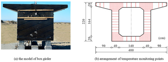
Figure 1.
The concrete box girder model.
After completing the fabrication of the model, thermal insulation and sealing treatment were applied to both ends of the beam to simulate negligible wind velocity conditions inside the bridge cavity under actual engineering conditions. The model utilized C55 concrete [24] with a water–cement ratio of 0.31, as well as an added water-reducing agent. Experimental tests revealed that at 7 days and 28 days, the compressive strengths of the standard cubic specimens were 59.8 MPa and 65.9 MPa, respectively.
2.2. Measuring Point Arrangement
The arrangement of sensors inside the box girder section is illustrated in Figure 1b. To accurately capture the temperature gradient, the sensors are densely positioned at the corner haunches of both the top and bottom girders, with a spacing of 6 cm between adjacent sensors. Considering minimal temperature variation in the web plate, a spacing adjustment to 15 cm is made between the measuring points. The sensor positions are adjusted according to reinforcement placement, and each individual sensor’s measuring point position is meticulously corrected prior to concrete pouring.
Additionally, a meteorological station was established within the experimental area to collect real-time meteorological data for the tested model. The station is equipped with sensors measuring atmospheric temperature and humidity and wind speed and direction, as well as a solar radiation meter. Data collection occurs at a sampling frequency of 1/60 Hz.
2.3. Meteorology Variation Due to Cold Wave Event
According to the characteristics of the diurnal temperature variation curve, the period from the time of reaching the daily maximum temperature until the following day’s minimum temperature is defined as the cooling period. The formula for calculating the magnitude of temperature cooling ΔTi during each cooling period is as follows:
where Timax is the maximum temperature of day i; T(i+1)min is the minimum temperature of day i + 1.
Based on atmospheric temperature data collected from 1 January 2017 to 30 January 2018, the magnitude of temperature cooling in the high-latitude region of northern Xinjiang was calculated using Equation (1). Subsequently, an extreme value analysis (EVA) was conducted on the temperature data to obtain the generalized extreme value (GEV) distribution. GEV distribution is a unified expression of Gumbel distribution, Fréchet distribution, and Weibull distribution. The cumulative distribution function (CDF) H(TD, μ, σ, k) is as follows [25]:
where u, σ, k represents location parameter, scale parameter, and shape parameter, respectively. TD represents the magnitude of temperature cooling (ΔTi), which was determined using Equation (1). Through fitting the temperature data, the coefficients u, σ, and k were determined to be 7.961, 4.916, and −0.249, respectively.
The frequency histogram of temperature cooling magnitudes and its probability density function are presented in Figure 2, illustrating the annual distribution. By fitting an extreme value distribution function and employing the statistical analysis theory for extreme value analysis [26], it is predicted that a once-in-50-year cold wave event in this region would result in a temperature decrease of 26.42 °C. Considering January as the month with the lowest average temperature during winter, this study focuses on the week from 11 to 17 January, depicting local meteorological conditions during this period in Figure 3. As depicted in Figure 3, the average weekly temperature significantly drops to 16.04 °C. Notably, there are three distinct periods of significant temperature drop around 13, 15, and 16 January, which have been categorized into three stages of cooling, as shown in Table 1. Among these stages, stage II exhibits the most substantial decrease with a magnitude of −18.39 °C, lasting for approximately 13.30 h; its recurrence period is calculated to be approximately every 49.76 days. Concurrently, solar radiation intensity reaches its peak value at 356.97 W/m² on 14 January at 13:48 during stage II of cooling, while strong winter winds prevail, with a maximum speed recorded as Level 7 (16.92 m/s) on 11 January at 14:32.
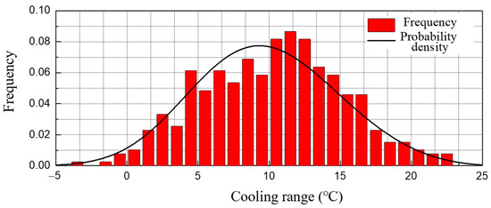
Figure 2.
Frequency histogram and fitting probability density function of temperature cooling amplitude.
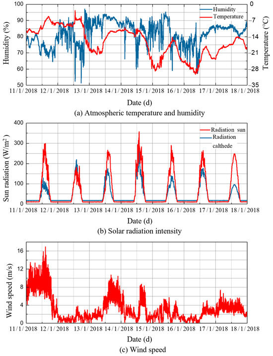
Figure 3.
Meteorological data.

Table 1.
Temperature cooling stages.
3. Temperature Testing Results of Concrete Box Girder
3.1. Temperature Time-Varying Rules
A local coordinate system is established on the measured cross-section based on the relative position of the sensors to determine the coordinates of each temperature measurement point and establish the coordinate index of the temperature sensors. The triangular meshing of the box girder’s cross-section is performed using a Delaunay triangulation algorithm, as shown in Figure 4. This algorithm ensures that no circumscribed circle of any triangular mesh overlaps with other measuring points [26,27]. By employing the finite element method with Lagrange shape function [28], interpolation and transformation are used to determine the temperature at arbitrary positions on the cross-section, thereby establishing a comprehensive database for measured temperature field across the entire cross-section. A temperature nephogram depicting the three stages of the box girder’s cross-section is illustrated in Figure 5.
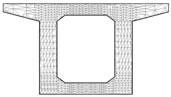
Figure 4.
Triangulation of the concrete box girder.
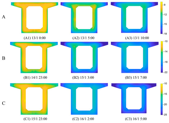
Figure 5.
Temperature nephogram of box girder at three stages.
Based on the measured temperature data across the cross-section of the box girder, it is postulated that each measurement point represents an approximation of the average temperature within its corresponding triangular area. Consequently, a weighted calculation formula for determining the average temperature of the cross-section is proposed as follows:
where denotes the mean temperature across the cross-section of the box girder; Ti represents the measured temperature value at the i-th temperature measurement point; Ai is the area represented by this measurement point; and n is the number of temperature measurement points.
The curve in Figure 6 illustrates the temperature evolution of the box girder cross-section obtained by solving Equation (3). It is evident that the temperature variation curve exhibits noticeable fluctuations, while the temperature reduction curve of the concrete box girder remains remarkably smooth. As abrupt drops occur in air temperature, three significant cooling stages can be observed across the average temperature of the box girder’s cross-section, as listed in Table 2. A comparison between Table 1 and Table 2 reveals a lag in cooling for the box girder’s cross-section following an abrupt drop in air temperature, with phase differences ranging from 0.23 h to 3.28 h. Notably, cooling stage I displays the smallest phase difference, whereas stage II exhibits the largest discrepancy. In stage I, temperature reduction commences at 17:46, when solar radiation intensity is relatively weak and has minimal impact on the box girder’s temperature field. Conversely, stage II experiences a rise in temperatures starting at 12:43, when solar radiation values are high and steadily increasing. During this stage, solar radiation energy is absorbed by the box girder model, leading to the continuous elevation of cross-sectional temperatures and resulting in a larger phase difference. These findings highlight that solar radiation significantly influences the temporal disparity between air temperature reduction and box girder cooling. A noticeable difference can be observed in the termination times of air temperature reduction, whereas the cross-sectional temperature of the box girder initiates an upward trend at around 10:00 in the morning. Research findings indicate that, in this region, sunrise occurs at approximately 10:00 a.m. during January. Following sunrise, the concrete box girder undergoes heat absorption due to solar radiation influence, leading to the cessation of cooling. Moreover, within the same cooling stage, the maximum temperature of the concrete box girder remains lower than that of ambient air temperature; however, its minimum temperature surpasses that of ambient air temperature. The discrepancy between their respective maximum values ranges from 0.49 °C to 2.48 °C, while for their minimum values, it varies from 8.10 °C to 10.66 °C. In summary, there exists a smaller cooling amplitude for the box girder compared to ambient air temperature, with a difference approximating 10.34 °C.
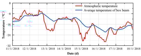
Figure 6.
Temperature time-varying curve.
Table 2.
Cooling stage of box girder section.
3.2. Temperature Distribution Rules
Based on the measured temperature values of the concrete box girder, vertical temperature distribution curves were plotted for each cooling stage on both the east and west side webs, as shown in Figure 7 and Figure 8. It can be observed that there is a characteristic time difference of 1 h between the east and west webs at each cooling stage, with the east side entering the cooling section first. Although there is only a small temperature change range in the web plate during all three stages, significant changes are observed in both the top and bottom plates, indicating that cooling has little effect on temperature changes along the thickness direction of concrete box girders.
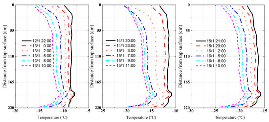
Figure 7.
Vertical temperature distribution of box girder in cooling stages I~III on the west side.
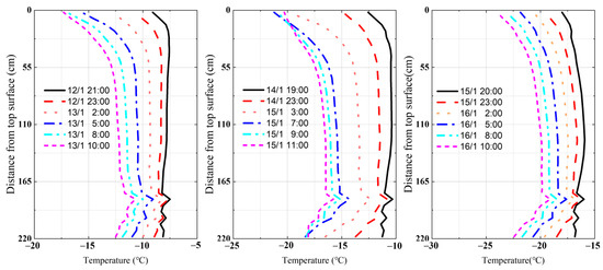
Figure 8.
Vertical temperature distribution of box girder in cooling stages I~III on the east side.
4. Numerical Simulation of Temperature Field
4.1. Finite Element Model
The temperature distribution of concrete box girders is commonly assumed to be uniform along the span direction due to natural environmental factors. When analyzing the temperature field using the general finite element program ABAQUS 6.14, it is presumed that the temperature remains constant across the longitudinal section. In other words, a two-dimensional heat conduction problem is established for conducting long-term numerical simulations on the test section. The differential equation for heat conduction can be expressed as follows:
where T represents the variation in temperature with respect to the structural coordinates, ρ is the density of concrete, c is the specific heat capacity, λ is the thermal conductivity, t is the time, and x, y are the structural coordinates. To obtain a finite solution for Equation (4), appropriate initial and boundary conditions are required. The initial condition refers to the temperature distribution of concrete at the beginning of analysis, which, in this study, was determined based on the daily average temperature at the location of the concrete box girder. On the other hand, boundary conditions represent external influences that affect heat conduction and temperature distribution within the box girder. Under solar radiation effects, three types of heat exchange between the bridge and the surrounding environment are considered: solar radiation heat flux, convective heat flux, and radiative heat flux. The thermal boundary conditions can be expressed as follows:
where qs, qr, and qc represent the heat flux densities of solar radiation, radiative heat transfer, and convective heat transfer, respectively. The convective heat transfer between the box girder and the atmosphere is considered as the third boundary condition. The solar radiation heat transfer and long-wave radiative heat transfer between the structure itself and the surrounding environment are treated as the second boundary conditions. During the finite element analysis process, it is necessary to convert the mixed boundary conditions into the third boundary conditions to obtain comprehensive values for the heat transfer coefficient and atmospheric environment temperature. These values are then introduced into FEM calculations. Equation (5) is reformulated as follows:
where Ta* represents the comprehensive atmospheric temperature, which is determined by the atmospheric temperature Ta, the solar radiation intensity perpendicular to the irradiated surface Iϕ, the radiative heat transfer coefficient hr, the convective heat transfer coefficient hc, and the solar radiation absorptivity α. Detailed calculations for radiation intensity and thermal boundary conditions can be found in reference [29]. For the finite element simulation of the box girder, a concrete box girder is modeled using four-node linear heat transfer quadrilateral elements (DC2D4). The mesh division of the model is illustrated in Figure 9. The thermal properties of the concrete in the segment model are listed in Table 3.

Figure 9.
Meshing.
Table 3.
Thermal properties of materials.
4.2. Model Validation
The model’s measurements and numerical simulation results are presented in Figure 10, illustrating the consistent temperature trends observed at different time intervals between the numerical simulation and measurements. Minor discrepancies exist at each data point, with a maximum difference of only 1.6 °C, which satisfies the precision requirements for engineering purposes. Thus, this analysis demonstrates that numerical simulation ensures the accurate representation of concrete box girder temperatures and faithfully reflects real-world conditions.
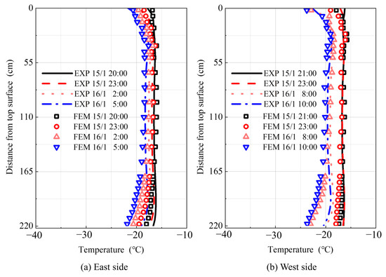
Figure 10.
Finite element temperature versus measured temperature.
5. Vertical Temperature Gradient Pattern of Concrete Box Girders under Cold Wave Action
5.1. Vertical Temperature Gradient Curve
Considering the vertical temperature distribution characteristics of concrete box girders, apart from the abrupt changes in localized temperature at the web corners of the bottom plate, particular attention is focused on the temperature difference gradient observed at the top plate. The formula for calculating the measured vertical temperature differential is defined as follows:
where ΔTtest represents the vertical measured temperature differential; Ttop denotes the measured temperature at measurement point No.1 on the top plate; Tfmax is the maximum temperature among the measurements in the web plate.
The time-varying pattern of the measured temperature differentials can be observed by calculating the vertical temperature differentials at each stage, as depicted in Figure 11, Figure 12 and Figure 13.
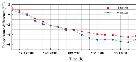
Figure 11.
Vertical measured temperature differential of box girder in cooling stage I.
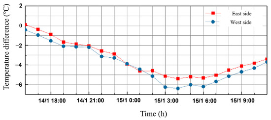
Figure 12.
Vertical measured temperature difference of box girder in cooling stage II.
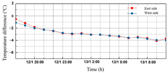
Figure 13.
Vertical measured temperature differential of box girder in cooling stage III.
The vertical negative temperature differentials on the east and west sides of the concrete box girder generally exhibit a continuous increase as the average temperature of the girder decreases, according to observations. The most unfavorable negative temperature differentials are typically observed approximately 1 h before reaching the minimum average temperature. However, during box girder cooling stage II, there is a significant increase in these negative temperature differentials due to a substantial rise in ambient air temperature. This leads to a rapid increase in the upper surface temperature of the top plate while the web plate continues to decrease in temperature due to heat conduction effects, resulting in reduced vertical negative temperature differentials. The maximum measured vertical negative temperature differential within the box girder occurs at 4:00 a.m. on 15 January, with a value of 6.38 °C, as shown in Figure 14. Based on an analysis of distribution characteristics for the top plate, bottom plate, and web plate’s respective curves for vertical negative temperature differentials, it is found that their distribution closely follows a combined exponential function:
where ΔT represents the vertical temperature gradient model of the concrete box girder; T1 stands for the temperature differential between the top plate and the web plate; T2 denotes the temperature differential between the bottom plate and the web plate; H is the height of the box girder; and y is the distance from the top plate’s upper surface to the measuring point. In this study, the most unfavorable negative temperature differentials were determined as T1= −7.5 °C for the top plate to the web plate and, simultaneously, T2 = −5 °C for the bottom plate to the web plate.
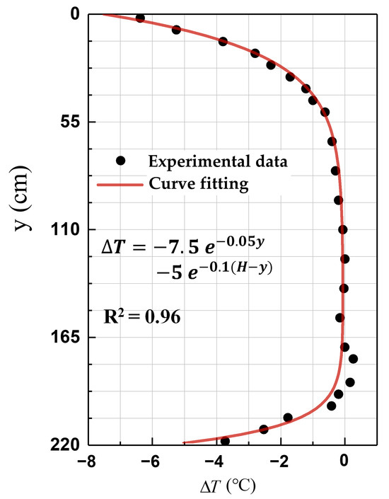
Figure 14.
The most unfavorable negative temperature differential fitting curve.
5.2. Temperature Gradient Extreme Value Analysis
5.2.1. Temperature Gradient Sample Data
To enhance the applicability and reliability of finite element simulation in practical engineering, in this study, we conducted two-dimensional heat conduction finite element simulations using historical meteorological data obtained from the “National Meteorological Science Data Center”. The data include total daily solar radiation, daily maximum/minimum temperatures, and daily average wind speeds. The selected period for analysis was 23 years, from 1993 to 2015, at the Xi’an (Jinghe) meteorological station. The extreme value analysis (EVA) was performed using a threshold model based on the Generalized Pareto (GP) distribution [30] to extract long-term daily extreme temperature differential samples induced by box girder temperature gradients. The probability density function is as follows:
where u is the threshold value and serves as the location parameter of GP distribution, while σ and k represent scale parameter and shape parameter, respectively. The type of GP distribution is determined by the value of k, where a value of 0 corresponds to GP type I distribution, positive values correspond to GP type II distribution, and negative values correspond to GP type III distribution.
For the top plate, there are 8400 samples available for each temperature differential. The data were sorted in descending order, and the top 4% of the data were chosen for threshold model analysis with the 336th data point as the threshold value. Similarly, corresponding bottom plate data from the top 4% were selected for threshold determination and extreme value analysis. Negative temperature differentials in cooling mode required calculation at extreme minimum values. Prior to conducting extreme value analysis, temperature effect sample data were multiplied by −1 to enable the calculation of representative values for temperature differentials using a method that finds extreme maximum values. Figure 15 presents samples of daily extreme temperature differentials spanning a period of 23 years from 1993 to 2015 with threshold values of u1 = 4.72 °C and u2 = 6.01 °C.
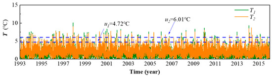
Figure 15.
Sample of T1, T2 in heating pattern (1993–2015).
5.2.2. Representative Value of Temperature Gradient Effect
The parameters for the GP distributions of various temperature differentials, estimated through distribution fitting analysis, are listed in Table 4. To demonstrate the effectiveness of the proposed GP distribution models, a Pearson χ2 test analysis was conducted at a significance level of α = 0.1 to fit the GP distribution. A probability density function comparison plot is illustrated in Figure 16. Based on this analysis, the representative values for T1 and T2 with a 50-year return period for the Xi’an box girder bridge were calculated as −10.54 °C and −9.44 °C, respectively. These values exhibit greater unfavorability compared to those obtained from the 23-year finite element calculations, thereby indicating reasonable agreement between the computed results.
Table 4.
GP distribution parameters and representative values of each temperature differential.
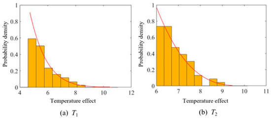
Figure 16.
Verification of GP distribution probability density function.
5.3. Vertical Temperature Gradient Pattern under Cold Wave Action
Actual temperature measurements provide a relatively accurate representation of the temperature distribution within the cross-section of the box girder, while the intricate nature of these distribution curves presents challenges in calculating, analyzing, and widely applying temperature differentials. Therefore, based on the morphology of the measured temperature field and referencing Chinese railway specifications and relevant literature, a simplified mathematical model for determining the temperature gradient of the box girder is proposed, as depicted in Figure 17. The formula for calculating the vertical temperature gradient is as follows:
where T1 and T2 represent the temperature differentials at the top and bottom surfaces, respectively; H stands for the beam height; and y denotes the distance from the top surface.
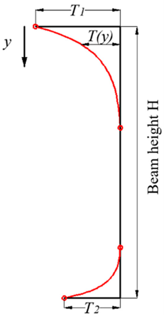
Figure 17.
Vertical temperature gradient mode (unit: cm).
6. Comparative Analysis with National Standards
6.1. Temperature Distribution Comparison
The axial expansion deformation, bending deformation, and generation of self-equilibrating stresses in concrete box girder structures are significantly influenced by the vertical temperature gradient resulting from a sudden decrease in temperature. Therefore, to validate the applicability of the proposed model, a comparative analysis was conducted among three codes—the General Code for Highway Bridge and Culvert Design (JTGD60-2015) [31], AASHTO LRFD bridge design specification (AASHTO) [32], and the British Code (BS5400) [33]—as illustrated in Figure 18. It can be observed that the vertically oriented temperature gradient model presented in this paper is 1.96 °C lower than JTGD60-2015 at the top of the box girder. However, it differs from the AASHTO and BS5400 specifications by 2.96 °C and 2.06 °C, with standard deviations of 0.873 and 0.451, respectively. At the bottom of the box girder, significant deviations are observed between the model proposed in this paper and the existing specifications. While JTGD60-2015 and AASHTO neglect temperature differentials at this location, they exhibit similar temperature distribution patterns which differ from those specified by BS5400. In contrast, the proposed model aligns closely with BS5400 at the bottom, with a difference of 3 °C and a standard deviation of 0.508. Therefore, the temperature gradient model effectively incorporates the gradient models specified by the JTGD60-2015, AASHTO, and BS5400 codes, ensuring bridge engineering safety in high-altitude and cold regions.
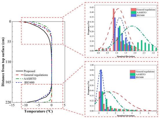
Figure 18.
Comparison of negative temperature gradient mode.
6.2. Temperature Self-Equilibrating Stress Comparison
To comprehensively analyze the influence of temperature effects on structural integrity, the European code categorizes the arbitrary temperature action on bridge sections into four components: effective temperature Te, vertical equivalent linear temperature difference Tv, horizontal equivalent linear temperature difference Th, and residual temperature distribution Tr. Among these components, both the vertical equivalent linear temperature difference Tv and residual temperature distribution Tr significantly impact concrete structures. Therefore, a comparison was made between the obtained vertical distribution of Tr by decomposing reference [34] and the above specifications, as shown in Figure 19. It is evident that both the proposed cooling model and the specifications exhibit consistent trends in terms of residual temperature distribution patterns. In all cases, negative values are observed at the top and bottom of the box girder, while positive values are found in its middle section. This indicates that compressive stresses are generated near the top and bottom of the box girder, whereas tensile stresses occur in its web plate. The residual temperature at the top surface of the cooling model presented in this paper is −5.36 °C, slightly higher than AASHTO’s specified value of −4.95 °C and BS5400’s specified value of −5.05 °C but still lower than JTGD60-2015’s specified value of −8.15 °C. In conclusion, there is only a marginal difference between the proposed formula and BS5400, as indicated by a standard deviation of 0.387; nevertheless, it exhibits substantial divergence from JTGD60-2015. This inconsistency can be attributed to the amplified temperature differential at the upper section under JTGD60-2015’s cooling mode and its subsequent influence on fluctuations in beam elevation.
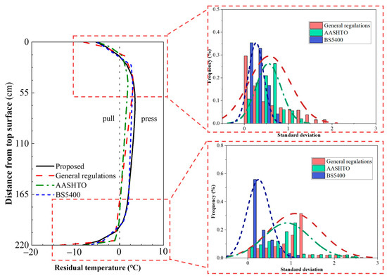
Figure 19.
Comparison of residual temperatures of box girder.
6.3. Temperature Curvature Comparison
The comparison of Tv derived from the various temperature gradient models with the maximum vertical linear negative temperature differential Tv, max obtained from measurements is illustrated in Figure 20. It can be observed that the temperature gradient proposed in this study exhibits a maximum negative temperature differential of −4.0 °C, deviating by +0.7 °C compared to Tv,max. This finding aligns more consistently with the values specified in current standards. In JTGD60-2015, the specified Tv of −5.3 °C exceeds the measured maximum negative temperature differential by +2.0 °C. AASHTO and BS5400 prescribe smaller Tv values compared to Tv, max, with differentials of −0.4 °C and −1.7 °C, respectively. Tv directly influences temperature-induced bending moments in bridges. While employing the temperature gradient model from JTGD60-2015 can encompass the effects of such moments, it often proves excessively conservative, resulting in less cost-effective bridge designs. Conversely, utilizing the temperature gradient models from AASHTO and BS5400 fails to adequately account for actual temperature differentials, leading to overly aggressive designs and an increased risk of cracking during operational phases.
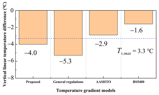
Figure 20.
Comparison of vertical linear temperature differentials of box girder.
7. Conclusions
The present study established a concrete box girder model in the severe cold region of northern Xinjiang, wherein 479 temperature sensors were installed to measure the temperature variations and distribution characteristics of temperature within the concrete box girder under the combined influence of low temperatures and cold wave cooling during winter. By fitting the measured temperature data, the most unfavorable vertical distribution pattern for negative temperature differentials was obtained. Additionally, an extreme value statistical analysis of atmospheric cooling amplitude was conducted based on 23 years of atmospheric temperature data. The following conclusions can be drawn:
- (1)
- Based on the results of rigorous statistical analysis, the estimated return period was found to be a mere 49.76 days. Furthermore, for a 50-year return period, the projected amplitude of temperature reduction during cold waves is expected to reach 26.42 °C, surpassing the worst-case measured temperature reduction by a factor of 1.44.
- (2)
- The vertical distribution curve of the most unfavorable negative temperature difference in concrete box girders within this experimental area can be described by a combined exponential function. Based on the measured data, a calculation formula for the temperature vertical gradient that is suitable for practical engineering applications was proposed. This formula effectively encompasses the specifications outlined in JTGD60-2015, AASHTO, and BS5400, thereby providing invaluable guidance for designing concrete bridges in cold regions.
- (3)
- The vertical distribution of residual temperature Tr and vertical linear temperature differential Tv in the cooling mode decomposition of this article is basically consistent with the specifications of JTGD60-2015, AASHTO, and BS5400. These results demonstrate that the temperature gradient model system proposed in this study is economically reasonable, mitigating the risk of bridge cracking during operation.
Author Contributions
Conceptualization, N.Z.; methodology, N.Z.; software, Y.-K.B. and H.L.; validation, N.Z.; formal analysis, H.L.; investigation, N.Z. and H.L.; resources, Y.-J.L.; data curation, Y.-K.B. and H.L.; writing—original draft preparation, H.L. and Y.-K.B.; writing—review and editing W.S. and N.Z.; supervision, Y.-J.L. and N.Z.; funding acquisition, H.L. and W.S. All authors have read and agreed to the published version of the manuscript.
Funding
This paper was funded by the Natural Science Basic Research Plan in Shaanxi Province of China (No. 2022JQ-475) and the National Natural Science Foundation of China (Grant No. 52208207, 52001052).
Institutional Review Board Statement
Not applicable.
Informed Consent Statement
Not applicable.
Data Availability Statement
The data that support the findings of this study are available from the corresponding author upon reasonable request.
Conflicts of Interest
The authors declare no conflicts of interest.
References
- Stewart, C.F. Long Structures without Expansion Joints; Caltrans: California Department of Transportation: Sacramento, CA, USA, 1967.
- Massicotte, B.; Picard, A.; Gaumond, Y.; Oullet, C. Strengthening of a long span prestressed segmental box girder bridge. PCI J. 1994, 39, 52–65. [Google Scholar] [CrossRef]
- Liu, Y.; Liu, J. Review on temperature action and effect of steel-concrete composite girder bridge. J. Traffic Transp. Eng. 2020, 20, 42–59. (In Chinese) [Google Scholar]
- Fan, L.; Guo, Y.; Zhao, Y.; Wang, T. Climate characterization of the severe cold weather in Altay region during 1962–2017. Desert Oasis Meteorol. 2020, 14, 92–98. (In Chinese) [Google Scholar]
- Bai, S.; Boernan, H.; Xie, X. The variation characteristics of cold wave in Altay prefecture under climate warming background. J. Glaciol. Geocryol. 2015, 37, 387–394. (In Chinese) [Google Scholar]
- Zhang, Q.; Li, J.; Singh, V.P.; Xiao, M. Spatio-temporal relations between temperature and precipitation regimes: Implications for temperature-induced changes in the hydrological cycle. Glob. Planet. Change 2013, 111, 57–76. [Google Scholar] [CrossRef]
- DelSole, T.; Shukla, J. Specification of wintertime North American surface temperature. J. Clim. 2006, 19, 2691–2716. [Google Scholar] [CrossRef][Green Version]
- Quesada, B.; Vautard, R.; You, P. Cold waves still matter: Characteristics and associated climatic signals in Europe. Clim. Chang. 2023, 176, 70. [Google Scholar] [CrossRef]
- Messori, G.; Faranda, D. On the systematic occurrence of compound cold spells in North America and wet or windy extremes in Europe. Geophys. Res. Lett. 2023, 50, e2022GL101008. [Google Scholar] [CrossRef]
- Song, Z.; Xiao, J.; Shen, L. On temperature gradients in high-performance concrete box girder under solar radiation. Adv. Struct. Eng. 2012, 15, 399–415. [Google Scholar] [CrossRef]
- Zhang, H.; Wang, P.; He, S.; Li, Y.; Chen, F.F.; Sun, N.N. Research of thermal effect of cable-stayed bridge with a separated side-box steel-concrete composite girder under solar radiation. Adv. Civ. Eng. 2021, 2021, 8812687. [Google Scholar] [CrossRef]
- Abid Sallal, R.; Tayşi, N.; Özakça, M. Temperature records in concrete box-girder segment subjected to solar radiation and air temperature changes. IOP Conf. Ser. Mater. Sci. Eng. 2020, 870, 012074. [Google Scholar] [CrossRef]
- Lee, J.; Kalkan, I. Analysis of thermal environmental effects on precast, prestressed concrete bridge girders: Temperature differentials and thermal deformations. Adv. Struct. Eng. 2012, 15, 447–459. [Google Scholar] [CrossRef]
- Roberts-Wollman, C.L.; Breen, J.E.; Cawrse, J. Measurements of thermal gradients and their effects on segmental concrete bridge. J. Bridge Eng. 2002, 7, 166–174. [Google Scholar] [CrossRef]
- Lu, Y.; Li, D.; Wang, K.; Jia, S. Study on solar radiation and the extreme thermal effect on concrete box girder bridges. Appl. Sci. 2021, 11, 6332. [Google Scholar] [CrossRef]
- Shen, Q.; Chen, J.; Yue, C.; Cao, H.; Chen, C.; Qian, W. Investigation on the through-thickness temperature gradient and thermal stress of concrete box girders. Buildings 2023, 13, 2882. [Google Scholar] [CrossRef]
- Abid, S.R.; Tayşi, N.; Özakça, M. Experimental analysis of temperature gradients in concrete box-girders. Constr. Build. Mater. 2016, 106, 523–532. [Google Scholar] [CrossRef]
- Li, H.; Zhang, Z.; Deng, N. Temperature field and gradient effect of a steel-concrete composite box girder bridge. Adv. Mater. Sci. Eng. 2021, 2021, 9901801. [Google Scholar] [CrossRef]
- Gu, B.; Chen, Z.; Chen, X. Temperature gradients in concrete box girder bridge under effect of cold wave. J. Cent. South Univ. 2014, 21, 1227–1241. [Google Scholar] [CrossRef]
- Larsson, O.; Thelandersson, S. Estimating extreme values of thermal gradients in concrete structures. Mater. Struct. 2011, 44, 1491–1500. [Google Scholar] [CrossRef]
- Nassar, M.; Amleh, L. The effect of projected air temperatures on concrete box girders thermal gradients and effective temperatures in Canada. Results Eng. 2023, 20, 101453. [Google Scholar] [CrossRef]
- Shi, T.; Sheng, X.; Zheng, W.; Lou, P. Vertical temperature gradients of concrete box girder caused by solar radiation in Sichuan-Tibet railway. J. Zhejiang Univ. Sci. A 2022, 23, 375–387. [Google Scholar] [CrossRef]
- Zhang, N.; Zhou, X.; Liu, Y.; Liu, J. In-situ test on hydration heat temperature of box girder based on array measurement. China Civ. Eng. J. 2019, 52, 76–86. (In Chinese) [Google Scholar]
- GB 50010–2010; Code for Design of Concrete Structures. China Architecture Publishing & Media Co., Ltd: Beijing, China, 2015.
- Liu, J.; Liu, Y.; Zhang, G. Experimental analysis of temperature gradient patterns of concrete-filled steel tubular members. J. Bridge Eng. 2019, 24, 04019109. [Google Scholar] [CrossRef]
- Wang, Y.; Ma, G.; Ren, F.; Li, T. A constrained Delaunay discretization method for adaptively meshing highly discontinuous geological media. Comput. Geosci. 2017, 109, 134–148. [Google Scholar] [CrossRef]
- Lee, D.; Schachter, B. Two algorithms for constructing a Delaunay triangulation. Int. J. Parallel Program. 1980, 9, 219–242. [Google Scholar] [CrossRef]
- El-Zafrany, A.; Cookson, R. Derivation of Lagrangian and Hermitian shape functions for triangular elements. Int. J. Numer. Methods Eng. 1986, 23, 275–285. [Google Scholar] [CrossRef]
- Liu, J.; Liu, Y.; Fang, J.; Liu, G.-L. Vertical temperature gradient patterns of I-shaped steel-concrete composite girder in arctic-alpine plateau region. J. Traffic Transp. Eng. 2017, 17, 32–44. (In Chinese) [Google Scholar]
- Liu, J.; Liu, Y.; Ma, Z.; Zhang, G.-J.; Lyu, Y. Temperature gradient action of steel-concrete composite girder bridge: Action pattern and extreme value analysis. China J. Highw. Transp. 2022, 35, 269–286. (In Chinese) [Google Scholar]
- JTG D60–2015; General Specifications for Design of Highway Bridges and Culverts. Ministry of Transport: Beijing, China, 2015.
- American Association of State Highway and Transportation Officials. AASHTO LRFD Bridge Design Specification; AASHTO: Washington, DC, USA, 2020. [Google Scholar]
- BS5400; Steel, Concrete and Composite Bridges, Part 2. Specification for Loads. Steel and Concrete Bridges Standards Committee: Washington, DC, USA, 1978.
- Chen, Q. Effects of Thermal Loads on Texas Steel Bridges. Ph.D. Thesis, The University of Texas, Austin, TX, USA, 2008. [Google Scholar]


Disclaimer/Publisher’s Note: The statements, opinions and data contained in all publications are solely those of the individual author(s) and contributor(s) and not of MDPI and/or the editor(s). MDPI and/or the editor(s) disclaim responsibility for any injury to people or property resulting from any ideas, methods, instructions or products referred to in the content. |
© 2024 by the authors. Licensee MDPI, Basel, Switzerland. This article is an open access article distributed under the terms and conditions of the Creative Commons Attribution (CC BY) license (https://creativecommons.org/licenses/by/4.0/).