Ride Comfort Prediction on Urban Road Using Discrete Pavement Roughness Index

Abstract

The prediction of ride comfort holds significant potential for enhancing the driving experience of both human drivers and autonomous vehicles, as it is closely correlated with pavement roughness. However, in urban road scenarios, the presence of shorter road segments and local irregularities introduces added complexity to ride comfort prediction. To better capture and characterize the irregularities and short road sections’ unevenness, we adopt the discrete roughness index (DRI) instead of the commonly used international roughness index (IRI) for assessing road profile unevenness, which is more suitable for urban roads. Ride comfort prediction is developed through numerical simulations using an eight-degree-of-freedom full-car model. The maximum transient vibration value (MTVV) is adopted to assess ride comfort. Through comparing the correlations between the MTVV and pavement roughness indices, it is indicated that the fitting degree of MTVV-DRI outperforms that of MTVV-IRI on short sections. Then, a set of speed-related DRI thresholds to estimate ride comfort distribution on a given road section is proposed, with considerations of vehicle speed, time period, and wheel paths. A hyperbolic-tangent-based speed control strategy is also proposed to avoid abrupt speed and acceleration changes during deceleration. This prediction method can assist drivers or autonomous vehicles in generating driving control strategies and maintaining a high level of ride comfort.

1. Introduction

Ride comfort is crucial to drivers and passengers as it is not only related to the ride quality but, more importantly, to driving safety and the health of drivers. On urban roads, short road segments and local irregularities further exacerbate ride discomfort. An effective and reliable prediction method of ride comfort will help drivers or autonomous vehicles improve riding experience and reduce the risk of accidents [1].

The prediction of ride comfort based on pavement roughness indices has been widely studied in recent decades because of their strong correlation [2,3,4]. Relative studies focused mainly on developing correlations between the ride comfort and the pavement roughness indices by means of simulations or field tests. In terms of ride comfort, the weighted root-mean-square acceleration (WRMSA) proposed in ISO 2631 [5] is the most commonly used index to characterize the effect of vibration on human comfort. WRMSA is capable of representing ride comfort over a relatively extended duration but struggles to characterize short-term ride comfort on brief road segments. In such instances, ISO 2631 also defines the maximum transient vibration value (MTVV) index for assessing transient vibration, which is better suited to evaluate ride discomfort resulting from road anomalies [6]. For pavement roughness, large amounts of indices have been proposed in past decades for the evaluation of roughness, taking into account vehicle–pavement interaction, the frequency contents of the road profile, and even road profile obstacles [7,8,9,10]. Among them, the international roughness index (IRI) [11] is recognized and used worldwide as a standard index for the evaluation of roughness. In addition, some other roughness indices or evaluation methods have also been made for specific scenarios, such as the bus ride index (BRI) for bus comfort evaluation [12], bicycle ride comfort evaluation [13], and the Being bump index (BBI) for airport pavement roughness evaluation [14]. Hettiarachchi et al. [15] provided a comprehensive summary of the prevalent indices utilized in pavement roughness evaluation, highlighting their respective properties. They underscored the significance of correlation adequacy with ride comfort, emphasizing its pivotal role in determining the applicability of a given roughness index.

Drawing upon findings from simulations or field measurements, extensive research efforts have been dedicated to the investigation of correlations aimed at ride comfort prediction [2,16,17,18]. Peter Múčka [19] summarized the relevant studies in the correlations proposed in the last twenty years and revealed the following: (1) the IRI is the most commonly used index for ride comfort prediction because of its strong linear relationship with the WRMSA; (2) ride comfort prediction accuracy is sensitive to vehicle speed, and higher speeds result in higher WRMSA. Though IRI is reliable to use to predict ride comfort, due to the specific definition of IRI, it is difficult to characterize the roughness of shorter road sections. Therefore, existing research mainly focuses on longer road sections (such as highways or expressways) and with less consideration of short road sections and urban roads. For example, the road surface is more uneven at the intersections as a result of the deceleration and the brakes of vehicles, whereas the pavement condition is better on other sections. Thus, the existing correlations may be inappropriate to predict the ride comfort on urban roads. Some scholars [20] have proposed using probability distribution indicators to characterize the fluctuation of driving comfort on road sections, but still cannot accurately predict local discomfort. Additionally, current studies rarely take the combined effects of the left and right wheel paths into consideration.

In the scenario of predicting ride comfort on urban short road sections, the main limitation of the IRI lies in its definition. The IRI is an average value that represents how significant the suspension response is at a particular distance. It performs well in long road sections (over 160 m) and high vehicle speeds [21], which determine a scenario of highways or freeways rather than urban roads whose road section is shorter and vehicle speed is non-uniform (ranges from approximately 20 to 100 km/h). However, the IRI can hardly provide sufficient details to identify localized features, while such local features may strongly diminish ride comfort. For instance, a single large event in a section of a smooth road can result in the same IRI as a road which has moderate events scattered throughout the road section, but the former road section would result in more discomfort. To break the limitations, Alvarez et al. [22] suggested the discrete roughness index (DRI). The DRI is a discrete indicator and calculated for each discretely measured location along with a road profile, which is more suitable to identify and characterize local features. The DRI also has an important property that the average value of converges to the IRI as the distance between sampled points becomes smaller. This indicates that the DRI characterizes pavement roughness without taking the distance of roads into account. Therefore, the DRI has great potential in ride comfort prediction, especially in road sections with unequal lengths.

The main objective of this paper is to propose a more reliable ride comfort prediction method on urban roads, and to prove that the novel roughness index, the DRI, is more appropriate for ride comfort evaluation. The comfort driving speed control strategies are also studied based on the prediction results. The remainder of this paper is organized as follows: the definitions of the two involved pavement roughness indexes (IRI and DRI) and the ISO ride comfort standard are presented in Section 2. Section 3 presents numerical analysis, including simulation model and data processing of the measured road profiles. In Section 4, we developed the correlations between the DRI and the MTVV by considering the speed, the time period, and the combined effect of the left and right wheel paths. The speed-related DRI thresholds and speed control strategy are also presented in this section. The final section summarizes the conclusions and future work.

2. Roughness Indexes and Ride Comfort Standard

2.1. International Roughness Index

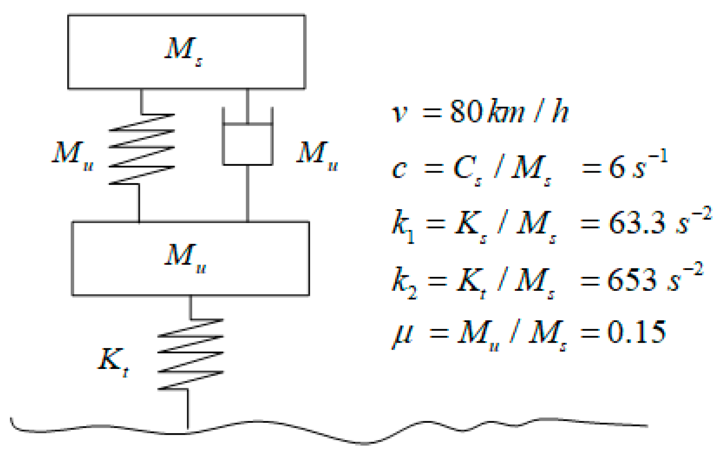
The IRI is calculated using a standard quarter-car model traveling on a single road profile at 80 km/h, as shown in Figure 1. The quarter-car model is characterized by five constants.

The mathematical expression of the IRI is shown in Equation (1) [11],

$$\mathrm{I}\mathrm{R}\mathrm{I}=\frac{1}{L}{\int }_0^T\left|\dot{z_s}-\dot{z_u}\right|dt$$

(1)

where $z_s$ and $z_u$ are the vertical motion for the sprung and unsprung masses in Figure 1. Due to the quarter-car model being a linear system, state space representation is introduced to solve the suspension response excited by a given road profile, as shown in Equation (2),

$$\left\{\begin{array}{c}\dot{\mathbf{x}}\left(t\right)=A\left(t\right)\mathbf{x}\left(t\right)+B\left(t\right)\mathbf{u}\left(t\right)\\ \mathit{y}\left(t\right)=C\left(t\right)\mathbf{x}\left(t\right)+D\left(t\right)\mathbf{u}\left(t\right)\end{array}\right.$$

(2)

where the vectors x, y, and u are the state vector, the output vector, and the input vector, respectively. The matrices A, B, C, and D are the state matrix, the input matrix, the output matrix, and the feedthrough matrix, respectively. For the quarter-car model, the state space equations can be written as Equations (3) and (4):

$$\left[\begin{array}{c}{\dot{z}}_s\\ {\ddot{z}}_s\\ {\dot{z}}_u\\ {\ddot{z}}_u\end{array}\right]=\left[\begin{array}{cccc}0& 1& 0& 0\\ -k_2& -c& k_2& c\\ 0& 0& 0& 1\\ \frac{k_2}{\mu }& \frac{c}{\mu }& \frac{-\left(k_1+k_2\right)}{\mu }& \frac{-c}{\mu }\end{array}\right]\left[\begin{array}{c}{z}_s\\ {\dot{z}}_s\\ z_u\\ {\dot{z}}_u\end{array}\right]+\left[\begin{array}{c}0\\ 0\\ 0\\ \frac{k_1}{\mu }\end{array}\right]z(t)$$

(3)

$${\dot{z}}_s-{\dot{z}}_u=\left[\begin{array}{cc}\begin{array}{cc}0& 1\end{array}& \begin{array}{cc}0& -1\end{array}\end{array}\right]\left[\begin{array}{c}{z}_s\\ {\dot{z}}_s\\ z_u\\ {\dot{z}}_u\end{array}\right]$$

(4)

Based on Equation (4), the IRI can be obtained by accumulating the suspension responses over the travel time. For typical paved roads, the IRI ranges from 0 to 12 m/km, where a low IRI indicates a smooth road profile and comfortable driving, whereas a high index indicates an uneven road profile.

2.2. Discrete Roughness Index (DRI)

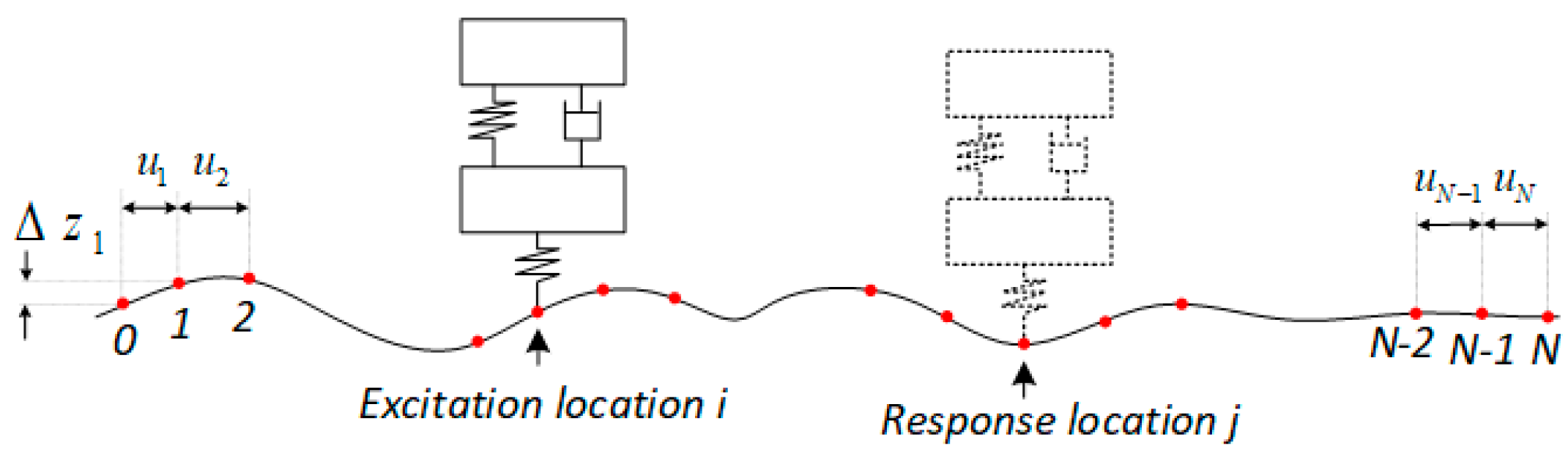
The DRI is also calculated based on the standard quarter-car model. As shown in Figure 2 [22], assuming that the vehicle response at the location point j is related to all the previous road profile excitation (location points 0~j − 1), then we define the fraction response at the point j of the excitation at the point i as the fractional response coefficient, $f_{ij}$, as shown in Equation (5),

$$f_{ij}=\left\{\begin{array}{cc}0& i>j\\ \frac{\left|\mathsf{\Delta }{z}_{i}h\left(t_j-t_i\right)\mathsf{\Delta }{t}_i\right|}{{\sum }_{k=1}^j\left|\mathsf{\Delta }{z}_{k}h\left(t_j-t_k\right)\mathsf{\Delta }{t}_k\right|}& i\le j\end{array}\right.$$

(5)

where $\mathsf{\Delta }{z}_i$ is the elevation difference between the point i and the i − 1; $\mathsf{\Delta }{t}_i$ denotes the corresponding time interval. The response function $h\left(t_j-t_i\right)$ denotes the response of the suspension travel at the time $t_j$ due to a unit impulse at the previous time $t_i$. Note that the sum of the coefficients of all the previous excitation points to the response the point j is equal to 1, as expressed in Equation (6).

$$\sum _{i=1}^N{f}_{ij}=1$$

(6)

The fractional response coefficient can be regarded as the contribution of the excitation at the point i to the response at the point j. Then, the DRI is defined as roughness attributable to a particular excitation, for a particular location point i, where the DRI is defined by Equation (7),

$${\mathrm{D}\mathrm{R}\mathrm{I}}_i=\sum _{j=1}^N\frac{1}{u_j}{f}_{ij}\left|{\dot{z}}_j\right|\Delta t_j$$

(7)

where ${\dot{z}}_j=\dot{z_s}-\dot{z_u}$ denotes the suspension responses at point j.

Compared with the IRI, the DRI is a series of discrete indicators characterizing the roughness of particular points. Moreover, it can be easily proved that the mean value of the DRI (DRIavg) converges to the IRI as the distance between the sampled points becomes smaller and the whole length of the road becomes larger, which is expressed by Equation (8),

$$\underset{\mathsf{\Delta }{u}_j\to 0}{\lim }DR{I}_{avg}=IRI$$

(8)

Therefore, the DRI can not only provide more details about the road profiles but also demonstrates the compatibility with the standard IRI measure. It is worth noting that the distance between the sampling points is an important factor in the calculation. Smaller distance provides more precise pavement roughness information but requires higher computational cost, while a longer distance has a lower computational cost but may neglect the local feature within a short distance.

2.3. Whole-Body Vibration

ISO 2631-1 [5] recommends the weighted root-mean-square acceleration (WRMSA) for evaluating human comfort and predicting health risk. The WRMSA is a comprehensive indicator taking into account the effects of frequency bands, positions, and acceleration directions. Since the uneven road affects the fluctuation of vertical vibration instead of longitudinal and transverse vibrations, we only consider the vertical vibration in this work.

The definition of WRMSA is expressed in Equation (9):

$$a_w={\left[\frac{1}{T}{\int }_0^T{a}_{wz}^2\left(t\right)dt\right]}^{\frac{1}{2}}$$

(9)

where T is the duration of the measurement and $a_{wz}$ is the vertical frequency-weighted acceleration, computed by Equation (10):

$$a_{wz}={\left[\sum _i{\left(W_i{a}_i\right)}^2\right]}^{\frac{1}{2}}$$

(10)

where W_i denotes the weighting factor for the i-th one-third octave band given in ISO 2631, and a_i denotes the vertical acceleration for the i-th one-third octave band. Moreover, since we mainly consider the pavement roughness of short road sections, the vibration in the vehicle appears to be more like a transient vibration. The ISO standard provides an index to describe transient vibration: the maximum transient vibration value (MTVV). The MTVV is defined based on the WRSMA and expressed in Equations (11) and (12).

$$a_w\left(t_0\right)={\left\{\frac{1}{\tau }\underset{t_0-\tau }{\overset{t_0}{\int }}{\left[a_{wz}\left(t\right)\right]}^{2}dt\right\}}^{\frac{1}{2}}$$

(11)

$$\mathrm{M}\mathrm{T}\mathrm{V}\mathrm{V}=\max \left[a_{wz}\left(t_0\right)\right]$$

(12)

where $a_{wz}\left(t\right)$ is the instantaneous frequency-weighted acceleration in the time domain, $t_0$ is the time of observation, and $\tau$ is the integration time for the moving average, and it is recommended to use $\tau =1$.

In

Table 1. Weighted acceleration and comfort levels.

Weighted Acceleration	Comfort Levels
Less than 0.315 m/s2	Not uncomfortable
0.315 m/s2 to 0.63 m/s2	A little uncomfortable
0.5 m/s2 to 1.0 m/s2	Fairly uncomfortable
0.8 m/s2 to 1.6 m/s2	Uncomfortable
1.25 m/s2 to 2.5 m/s2	Very uncomfortable
Greater than 2.0 m/s2	Extremely uncomfortable

, the ISO standard also provides the approximate indications of likely comfort reactions to vibration in public transport, which can be utilized to estimate the pavement roughness thresholds in the following sections.

3. Numerical Simulation

3.1. Vehicle Model

In the past decades, numerical simulation has been proven to be an effective approach for investigating the dynamic response of vehicles on an uneven road profile; many vehicle models were suggested, including the quarter-car model, the half-car model, and the full-car model. By using proper validated mechanical parameters, these multi-DOF (degree of freedom) models allow us to solve dynamic vehicle responses in both the time domain [23] and frequency domain [24].

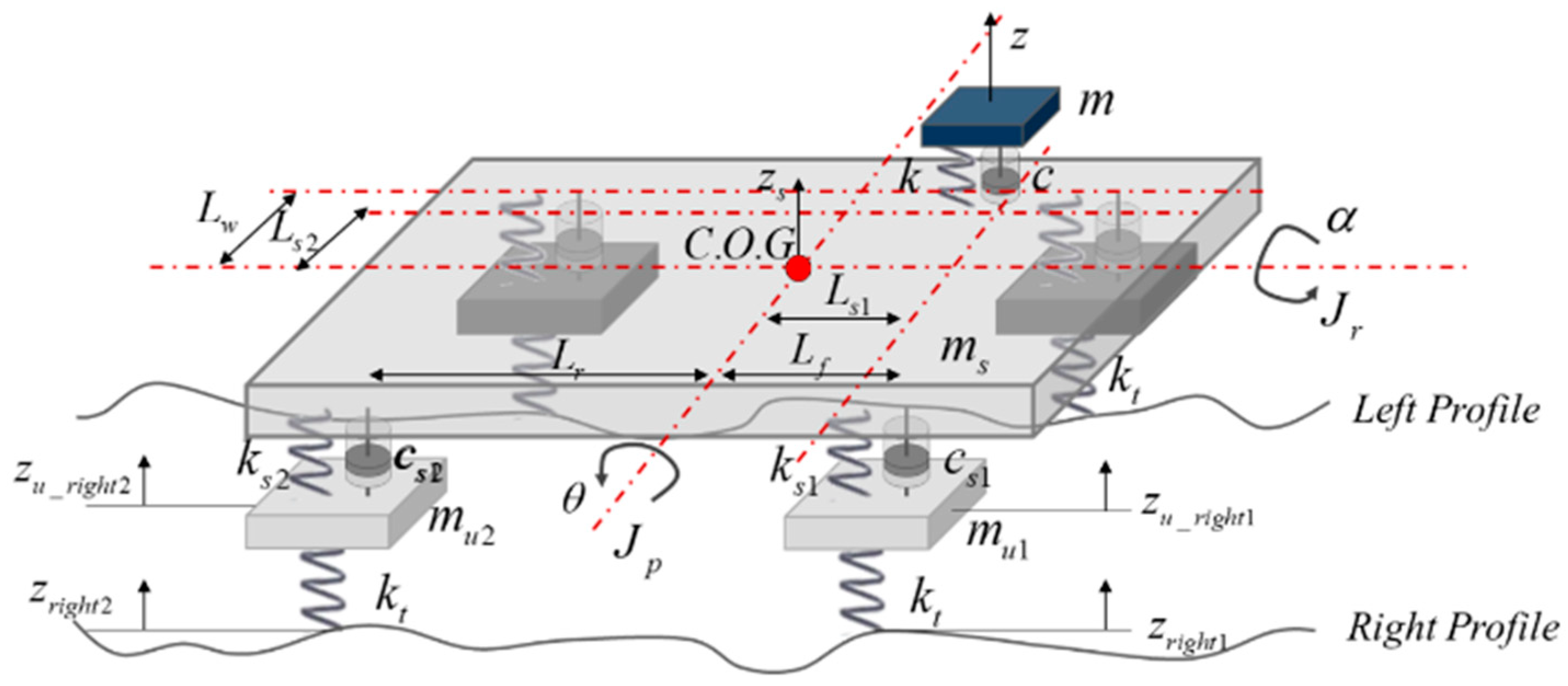
In this study, we focus mainly on the effect of pavement roughness on the whole-body vibration. Therefore, we adopted an eight DOF vehicle model, which was an extension of the quarter-car model, which allows us to extract the accelerations on different seats. The model parameters are referenced from lecture [19]. As shown in Figure 3, this model took the effects of both of the two uneven road profiles of the left and right wheel paths into consideration, which could better simulate the rolling and pitching motions of the vehicle. A degree of freedom for seat was defined in this model to solve the accelerations on the seat. The position of the seat can be adequately adjusted to match the position of drivers or passengers. Moreover, we assumed that the vehicle did not accelerate, brake, or steer during the simulation, and only the vertical responses of the seat were considered.

According to Newton’s law, the vibration of the full-car model is described in Equation (13).

$$\left[\mathbf{M}\right]\left\{\ddot{\mathbf{Z}}\right\}+\left[\mathbf{C}\right]\left\{\dot{\mathbf{Z}}\right\}+\left[\mathbf{K}\right]\left\{\mathbf{Z}\right\}=\left\{\mathbf{F}\left(t\right)\right\}$$

(13)

where $\ddot{\mathbf{Z}}$, $\dot{\mathbf{Z}}$, and $\mathbf{Z}$ are the acceleration vector, the velocity vector, and the displacement vector, M, C, and K are the mass matrix, the damping matrix, and the spring matrix, and $\mathbf{F}\left(t\right)$ represents the external force of the vibration system. Assuming that the road profiles of the right and left wheel paths are $z_1\left(t\right)$ and $z_2,\hspace{0.17em}\mathrm{r}\mathrm{e}\mathrm{s}\mathrm{p}\mathrm{e}\mathrm{c}\mathrm{t}\mathrm{i}\mathrm{v}\mathrm{e}\mathrm{l}\mathrm{y}$, F(t) can be written as Equation (14).

$$F\left(\mathrm{t}\right)=\left[\begin{array}{c}-k_t{z}_1\left(t\right)\\ -k_t{z}_2\left(t\right)\\ -k_t{z}_1\left(t-\frac{l}{v}\right)\\ -k_t{z}_2\left(t-\frac{l}{v}\right)\\ {\mathbf{0}}_{4\times 1}\end{array}\right]$$

(14)

Also, we obtained the state space representation of Equation (12), as expressed in Equations (15) and (16).

$$\left\{\begin{array}{c}\ddot{\mathbf{Z}}\\ \dot{\mathbf{Z}}\end{array}\right\}=\left[\begin{array}{cc}-{\mathbf{M}}^{-1}\mathbf{C}& -{\mathbf{M}}^{-1}\mathbf{K}\\ \mathbf{0}& \mathbf{I}\end{array}\right]\left\{\begin{array}{c}\dot{\mathbf{Z}}\\ \mathbf{Z}\end{array}\right\}+\left\{\begin{array}{c}{\mathbf{M}}^{-1}\\ \mathbf{0}\end{array}\right\}\mathbf{F}\left(t\right)$$

(15)

$$\ddot{\mathbf{Z}}=\left[\begin{array}{cc}-{\mathbf{M}}^{-1}\mathbf{C}& -{\mathbf{M}}^{-1}\mathbf{K}\end{array}\right]\left\{\begin{array}{c}\dot{\mathbf{Z}}\\ \mathbf{Z}\end{array}\right\}+\left[{\mathbf{M}}^{-1}\right]\mathbf{F}\left(t\right)$$

(16)

Assuming that the seat denotes the nth DOF, we can extract the vertical acceleration by the output of the nth element of the vector. The simulations are implemented on Matlab 2020b, with a time interval of 0.001 s.

3.2. Road Profile

To guarantee the reliability of the simulation results, we collected 108 real urban road profiles with an IRI range of 0.82~12.95 and a distance range of 58~1282 m. The elevations of the road profiles were captured by a laser-based profiler in Shanghai, China. The profiler was equipped with five laser sensors, and thus we could easily capture the road profiles of both the right and left wheel paths. During the measurement, the moving speed of the profiler was not fixed, meaning that the profile data were discrete and had an unequal space interval (about 0.1~0.3 m). Thus, a cubic spline interpolation method was first applied to obtain a uniform road profile, with a space interval of 0.01 m, which corresponded to the spatial frequency of 100 m⁻¹.

Prior to the simulation and further analysis, the original road profile data needed to be filtered because the raw data usually contained surface irregularities and cracks. To this end, Sayers [25] applied a 250 mm moving average filter to smooth the road profile, which was widely used in the current studies. Although this filter is suitable for the IRI calculation, it is not applicable to calculate the DRI because the moving average filter can hardly eliminate some sudden changes in the road profile. The DRI calculation is very sensitive to the emergent changes in the road profile, but the vertical acceleration of the seat is hardly influenced by such emergent changes. Since the road profile can be considered as the system excitation, and the vertical acceleration of the seat is regarded as the system response, we can obtain the corresponding frequency response function (FRF) at various speeds, as shown in Equation (17),

$$H\left({\omega }_s\right)=\frac{a_{seat}\left(\omega \right)}{z_{road}\left({\omega }_s\right)}$$

(17)

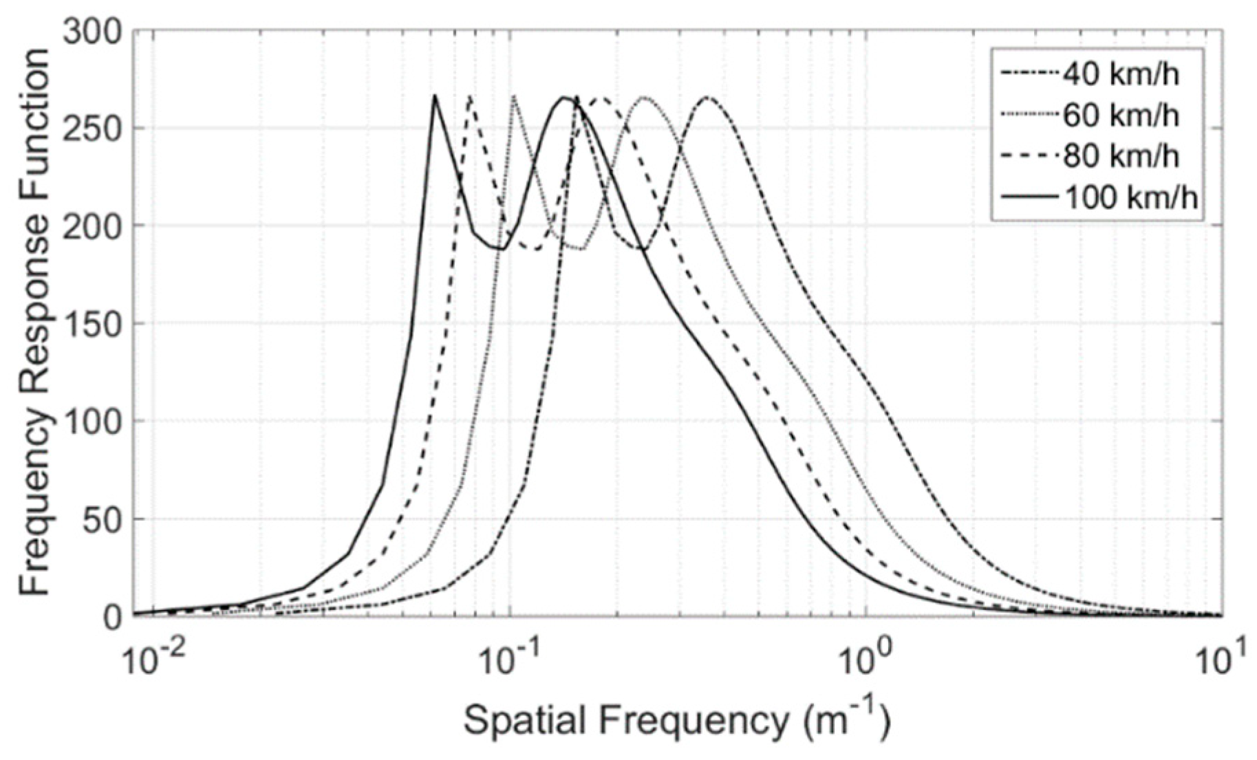
where $a_{seat}\left(\omega \right)$ and $z_{road}\left({\omega }_s\right)$ are the frequency spectrums of acceleration on the seat and the road profile, respectively. Note that the ${\omega }_s$ is spatial frequency, whose unit is ${\mathrm{m}}^{-1}$. By solving the response excited by a unit impulse of the road profile, FRF curves at different speeds are obtained (see Figure 4).

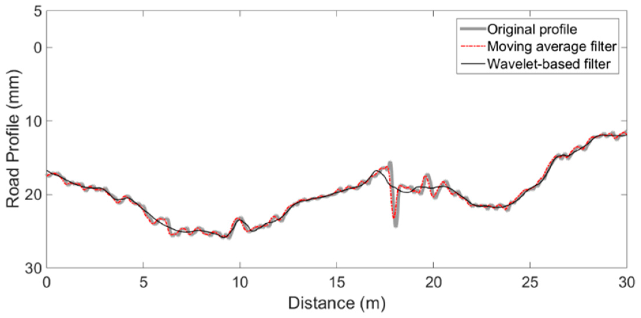
It is seen that the magnitudes of the frequency response function are mainly distributed in the spatial frequency range of [0, 6] ${\mathrm{m}}^{-1}$, which indicates a slight effect of high-frequency parts (over 10 m⁻¹) on the vertical acceleration of the seat. Therefore, we adopted a wavelet-based filter to smooth the original road profile. The original profile data were firstly decomposed using a five-level wavelet, and then the fifth component corresponding to the frequency bands of [0, 6.25] was selected as the smoothed data. Figure 5 shows the original profile and two smoothed road profiles using the moving average filter and wavelet-based filter, respectively. It is seen that the wavelet-based filter can effectively eliminate the abrupt change at around 17 m.

Next, the DRI and IRI values of the road profiles are computed and compared, as illustrated in Figure 6. It is noteworthy that the box plot illustrates the distribution of the DRI across each road section. It can be observed that road sections with higher IRI values exhibit a more scattered distribution of the DRI, indicating the presence of numerous localized irregularities in those sections. Moreover, even in road sections with lower IRI values, there are still some localized irregularities present. This suggests that the DRI is more sensitive to localized abnormal irregularities compared to the IRI.

4. Results

4.1. DRI and Ride Comfort

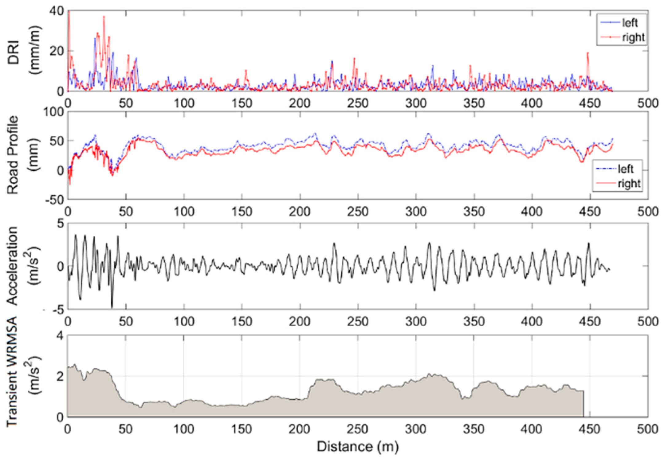
To study if the DRI can identify local features and characterize ride comfort, a 470 m long road section was selected as an example. The corresponding IRIs of the left and right wheel paths were 3.34 and 3.49, respectively. Considering the computational cost, we calculated the DRI on every 1.0 m long section. Figure 7 illustrates the DRI, the road profiles, and the vertical acceleration on the driver’s seat. The transient WRMSA (WRMSA in 1 s) curve is also plotted in Figure 6. Note that the simulation was implemented at a speed of 80 km/h.

Firstly, as shown in the section of 0~50 m, the corresponding DRI is much higher than the DRI in the other sections, and the corresponding acceleration also has a significant fluctuation. See the section of 70~180 m. The DRI is relatively small and corresponding to a flat road surface and a slight vibration. This demonstrates that the DRI can localize the uneven pavement profile and the violent vibration on the driver’s seat. Based on Equation (9), we can calculate the WRMSA of the whole section, which is $0.937\hspace{0.17em}\mathrm{m}/{\mathrm{s}}^2$, corresponding to the comfort level of “fairly uncomfortable”, while the transient WRMSA exceeds $0.937\hspace{0.17em}\mathrm{m}/{\mathrm{s}}^2$ at some locations. The transient WRMSA at the beginning and at around 300 m can reach 2.5 m/s² and 2.0 m/s², respectively, which both correspond to the comfort level of “very uncomfortable”. This indicates that the discomfort resulting from uneven short sections may be neglected if we only consider the ride comfort of driving on a long road section; thus, it is necessary to propose a new prediction method for the ride comfort in consideration of the effect of short sections.

4.2. Correlations between DRI and MTVV

Since the DRI can effectively identify the pavement roughness of short sections, it is possible to predict the short-time ride comfort by using the DRI. Based on the simulation results on the measured 108 urban road sections, the correlations between the DRI and MTVV were developed for ride comfort prediction. During the simulation, we considered three factors: the vehicle speed, the time period, and the combined effect of the left and right wheel paths.

4.2.1. Vehicle Speed

Research revealed that ride comfort was strongly related to vehicle speed [16]. Passengers suffer from more discomfort at a higher speed. For urban roads, vehicle speed has a wide range due to complex traffic conditions; hence, four different speeds are discussed in this study: 40, 60, 80, and 100 km/h.

4.2.2. Time Period

As the MTVV is defined as the maximum value within a certain period of time, the correlation between the MTVV and the DRI would be affected by the time period which determines the localization resolution of the ride comfort prediction. To study the effect of the time period, we discuss three different time periods in the simulation: 1, 2, and 4 s.

4.2.3. The Combined Effect of the Left and Right Wheel Paths

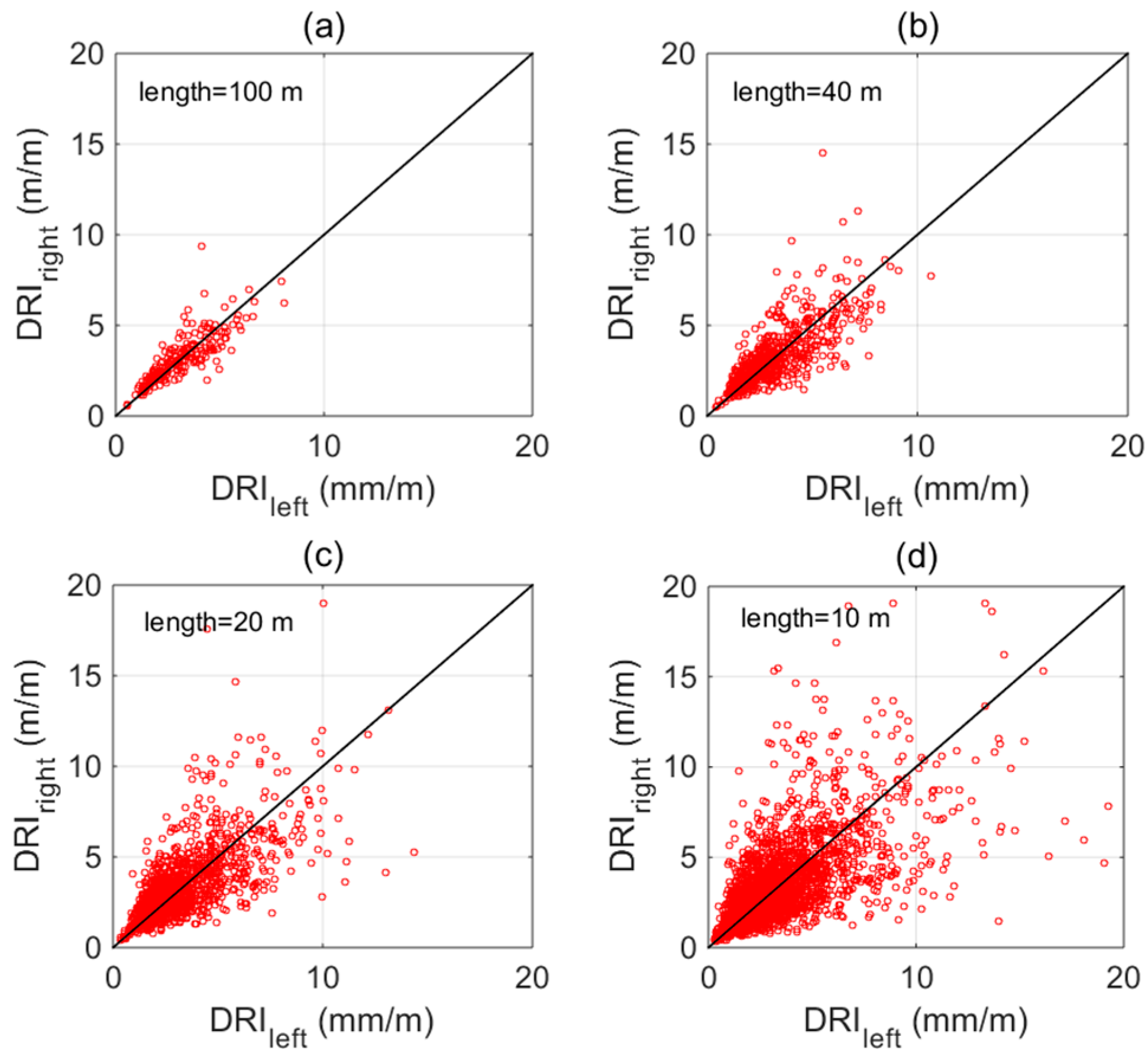
Similar to the IRI, the DRI can only reflect the pavement roughness of one single road profile, while actually the vibration in the vehicle is provoked by both the left and right wheel path. Many research employed the average IRI of the two profiles to consider the combined effect, which is reliable in long-road-section measurements but does not perform well in the measurement of short sections. Figure 7 shows the relations between the DRIleft and the DRIright in the cases of four different lengths of road sections. Note that the DRIleft and the DRIright are the mean value of the DRI of the left and right profiles, respectively.

Since the mean value of the DRI converges to the IRI when the whole length of the road section becomes larger, the DRI in Figure 8a, whose length of road is 100 m, is almost equal to the IRI. Therefore, the significant correlation between the DRIleft and the DRIright demonstrates the reliability of using the average IRI to characterize the pavement roughness of the whole road because the two profiles have close pavement roughness in long sections. On the contrary, for short-distance sections, there is a significant difference in the DRI calculated on the left and right wheel paths. As seen in Figure 8b–d, the correlation is becoming weaker as the length becomes shorter. While driving on short sections, any change in one side will affect the ride comfort on both sides. Generally, the left wheel path makes more contribution to the vibration of the driver’s seat (assuming that the driver’s seat is on the left), whereas the road profile on the right wheel path has more influence on the vibration of the passenger’s seat. Therefore, it is necessary to discuss the combined effect when studying the correlations between pavement roughness and ride comfort.

4.2.4. Correlation Development

In previous studies, it was widely accepted that the IRI has a good linear relation with the WRMSA. The DRI is more sensitive to the local unevenness than the IRI; however, the linear relation may not be suitable for developing correlations between the DRI and the MTVV. Therefore, we adopted the power function regression ($\mathrm{M}\mathrm{T}\mathrm{V}\mathrm{V}={\mathrm{a}}_1\mathrm{D}\mathrm{R}{\mathrm{I}}_{\mathrm{r}\mathrm{i}\mathrm{g}\mathrm{h}\mathrm{t}}^{{\mathrm{a}}_2}·\mathrm{D}\mathrm{R}{\mathrm{I}}_{\mathrm{l}\mathrm{e}\mathrm{f}\mathrm{t}}^{{\mathrm{a}}_3}$, a₁, a₂, a₃ are fitting parameters) to develop the correlations, summarized in

Table 2. Correlations of DRI_avg vs. MTVV and IRI vs. MTVV.

Time Period	Speed	DRI vs. MTVV	IRI vs. MTVV
1 s	40 km/h	$\mathrm{M}\mathrm{T}\mathrm{V}\mathrm{V}=0.23DR{I}_{left}^{0.62}·DR{I}_{right}^{0.22} R^2=0.63$	$\mathrm{M}\mathrm{T}\mathrm{V}\mathrm{V}=0.22IR{I}_{left}^{0.54}·IR{I}_{right}^{0.25} R^2=0.62$
	60 km/h	$\mathrm{M}\mathrm{T}\mathrm{V}\mathrm{V}=0.37DR{I}_{left}^{0.67}·DR{I}_{right}^{0.25} R^2=0.76$	$\mathrm{M}\mathrm{T}\mathrm{V}\mathrm{V}=0.34IR{I}_{left}^{0.66}·IR{I}_{right}^{0.21} R^2=0.74$
	80 km/h	$\mathrm{M}\mathrm{T}\mathrm{V}\mathrm{V}=0.49DR{I}_{left}^{0.62}·DR{I}_{right}^{0.29} R^2=0.74$	$\mathrm{M}\mathrm{T}\mathrm{V}\mathrm{V}=0.48IR{I}_{left}^{0.62}·IR{I}_{right}^{0.18} R^2=0.65$
	100 km/h	$\mathrm{M}\mathrm{T}\mathrm{V}\mathrm{V}=0.60DR{I}_{left}^{0.56}·DR{I}_{right}^{0.35} R^2=0.72$	$\mathrm{M}\mathrm{T}\mathrm{V}\mathrm{V}=0.60IR{I}_{left}^{0.55}·IR{I}_{right}^{0.22} R^2=0.60$
2 s	40 km/h	$\mathrm{M}\mathrm{T}\mathrm{V}\mathrm{V}=0.26DR{I}_{left}^{0.73}·DR{I}_{right}^{0.20} R^2=0.72$	$\mathrm{M}\mathrm{T}\mathrm{V}\mathrm{V}=0.23IR{I}_{left}^{0.72}·IR{I}_{right}^{0.17} R^2=0.71$
	60 km/h	$\mathrm{M}\mathrm{T}\mathrm{V}\mathrm{V}=0.41DR{I}_{left}^{0.78}·DR{I}_{right}^{0.24} R^2=0.80$	$\mathrm{M}\mathrm{T}\mathrm{V}\mathrm{V}=0.37IR{I}_{left}^{0.80}·IR{I}_{right}^{0.14} R^2=0.78$
	80 km/h	$\mathrm{M}\mathrm{T}\mathrm{V}\mathrm{V}=0.57DR{I}_{left}^{0.64}·DR{I}_{right}^{0.32} R^2=0.78$	$\mathrm{M}\mathrm{T}\mathrm{V}\mathrm{V}=0.55IR{I}_{left}^{0.50}·IR{I}_{right}^{0.36} R^2=0.70$
	100 km/h	$\mathrm{M}\mathrm{T}\mathrm{V}\mathrm{V}=0.69DR{I}_{left}^{0.57}·DR{I}_{right}^{0.40} R^2=0.76$	$\mathrm{M}\mathrm{T}\mathrm{V}\mathrm{V}=0.68IR{I}_{left}^{0.43}·IR{I}_{right}^{0.40} R^2=0.64$
4 s	40 km/h	$\mathrm{M}\mathrm{T}\mathrm{V}\mathrm{V}=0.29DR{I}_{left}^{0.78}·DR{I}_{right}^{0.22} R^2=0.76$	$\mathrm{M}\mathrm{T}\mathrm{V}\mathrm{V}=0.27IR{I}_{left}^{0.67}·IR{I}_{right}^{0.27} R^2=0.74$
	60 km/h	$\mathrm{M}\mathrm{T}\mathrm{V}\mathrm{V}=0.47DR{I}_{left}^{0.82}·DR{I}_{right}^{0.24} R^2=0.83$	$\mathrm{M}\mathrm{T}\mathrm{V}\mathrm{V}=0.42IR{I}_{left}^{0.57}·IR{I}_{right}^{0.43} R^2=0.80$
	80 km/h	$\mathrm{M}\mathrm{T}\mathrm{V}\mathrm{V}=0.64DR{I}_{left}^{0.72}·DR{I}_{right}^{0.29} R^2=0.78$	$\mathrm{M}\mathrm{T}\mathrm{V}\mathrm{V}=0.59IR{I}_{left}^{1.15}·IR{I}_{right}^{-0.23} R^2=0.72$
	100 km/h	$\mathrm{M}\mathrm{T}\mathrm{V}\mathrm{V}=0.81DR{I}_{left}^{0.66}·DR{I}_{right}^{0.34} R^2=0.76$	$\mathrm{M}\mathrm{T}\mathrm{V}\mathrm{V}=0.77IR{I}_{left}^{0.73}·IR{I}_{right}^{0.16} R^2=0.67$

, and the regressed correlations between the IRI and the MTVV were also calculated and summarized for comparison. Once the correlations were developed, we could easily predict the ride comfort on the road sections with the given profile.

From Table 2, we can see that the performance of the DRI-based prediction method outperforms the IRI-based method. The R-squares of the DRIavg vs. $\mathrm{M}\mathrm{T}\mathrm{V}\mathrm{V}$ are mostly higher than those of the IRI, especially at a high speed. This indicates that the DRI is more applicable to predict ride comfort. The exponents of the DRIleft and the DRIright indicate how significant their effects are. It is observed that the exponents in the correlations of the DRI vs. MTVV follow this trend: as the vehicle speed increases, the exponent of the DRIright grows continuously. It can be concluded that the left and right wheel paths both have a significant effect on the ride comfort at a high speed, while the ride comfort is mainly affected by the closest wheel path at a low speed.

It is also observed that the fitting performance becomes better at longer time periods. The highest R-square only reaches 0.76 when the time period is 1 s. Therefore, we adopted the time period of 2 s and the corresponding MTVV-DRI correlations to propose speed-related pavement roughness thresholds.

4.3. Speed-Related Pavement Roughness Threshold

To identify if a road is smooth enough to ensure ride comfort for vehicles, we determined the speed-related pavement roughness thresholds based on the whole-body vibration limits (shown in Table 1) and the correlations in Table 2. These thresholds can guide drivers or autonomous vehicles to adjust their speeds to improve ride comfort.

The correlations in Table 2 only focus on driver’s ride comfort; the passengers’ comfort should also be considered. As the position of the passenger seat is symmetrical to the position of the driver’s seat and the parameters of the two seats are almost identical, we can easily obtain the correlations between the DRI and the ride comfort on the passenger seat by switching the variables of the DRIleft and the DRIright. For example, the correlation for the driver’s seat at 80 km/h in 2 s is ${\mathrm{a}}_{\mathrm{w}\mathrm{z}}=0.57DR{I}_{left}^{0.64}·DR{I}_{right}^{0.32}$; then, we can find the correlation for the passenger seat:

$$\mathrm{M}\mathrm{T}\mathrm{V}\mathrm{V}=0.57DR{I}_{right}^{0.64}·DR{I}_{left}^{0.32}$$

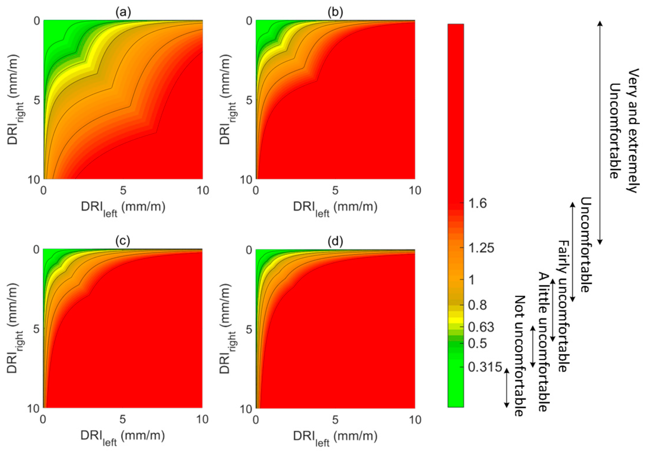
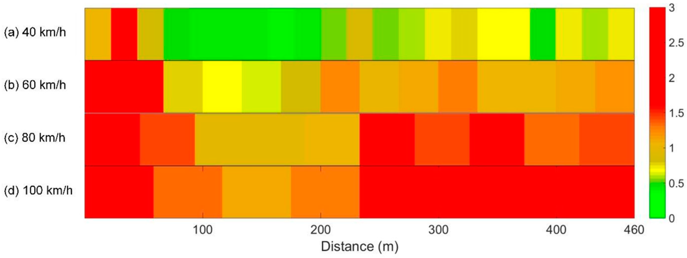
On the basis of the correlations of the two seats and the vibration limits in Table 1, we finally determine the pavement roughness thresholds at different speeds. Figure 9 provides the DRI thresholds, which can be devoted to evaluating and predicting the ride comfort on short road sections. The color scale indicates the comfort level, and the black lines clearly show the DRI thresholds corresponding to the vibration limits marked on the right color bar.

4.4. Application for Ride Comfort Prediction and Speed Control

For a given road section with known profiles, we can easily predict the ride comfort based on the DRI calculation and the correlations in Table 2. During the ride comfort prediction, it is necessary to first define the road segmentation method and the vehicle speed. By using the 2 s-MTVV to represent the ride comfort, we can obtain a “map” showing how the ride comfort is distributed over the whole section at a fixed speed, as shown in Figure 10.

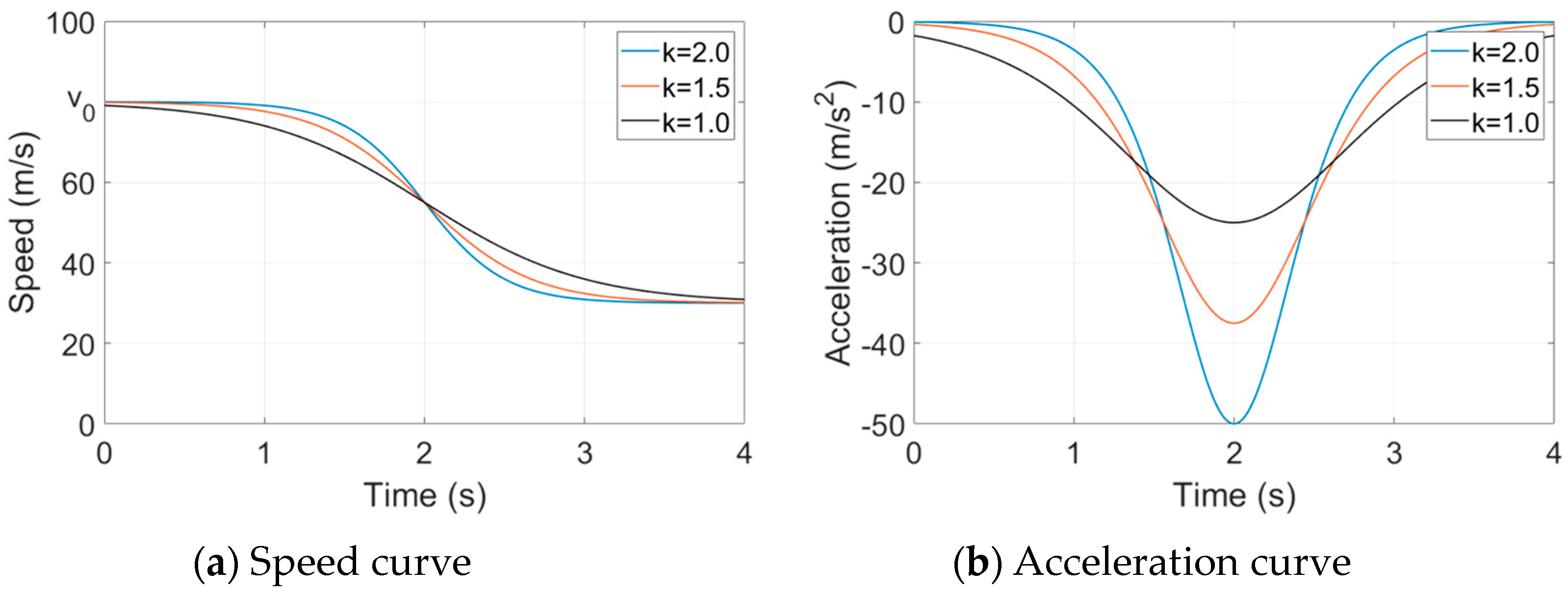
Note that the road section in Figure 9 is the same as the road section in Figure 6. The color scale along the distance indicates ride comfort. The ride comfort prediction results can guide us in developing a speed control strategy to avoid severe turbulence. To maintain a good comfort level, vehicles can decelerate on rough road sections and accelerate on flat sections. As the deceleration and acceleration of a vehicle also induce discomfort, we adopted a hyperbolic tangent curve to generate the speed control strategy [26]:

$$v=-\frac{b}{2}\tanh \left(k\left(t-p\right)\right)-\frac{b}{2}+v_0$$

(18)

where v₀ indicates the initial speed, t denotes the time, v is the targeted speed, $b=v_0-v$, p is a model constant, and k is the stability coefficient that determines the curve of the speed changes. By calculating the differentiation of Equation (18), the expression of the acceleration of the vehicle is as follows (Figure 10b):

$$a_{longi}=-\frac{bk}{2}\left(1-{\left(\tanh \left(k\left(t-p\right)\right)\right)}^2\right)$$

(19)

$$\max \left(a_{longi}\right)=\frac{b·k}{2}$$

(20)

The hyperbolic tangent curve resembles the process of human deceleration or acceleration, as shown in Figure 11. In practice, we care more about the deceleration stage because vehicles allow us to brake suddenly, but sudden acceleration is usually not allowed. Therefore, we only consider the deceleration stage in this study.

As expressed in Equations (19) and (20), the stability coefficient k is the key factor that affects the acceleration of vehicles. To maintain a good comfort level during deceleration, vehicles should select a small k to avoid sudden changes in speed and acceleration. Then, combining the vertical acceleration with the longitudinal acceleration, we can calculate the combined maximum transient acceleration (MTVV_cob) based on ISO 2631, expressed as follows:

$${\mathrm{M}\mathrm{T}\mathrm{V}\mathrm{V}}_{\mathrm{c}\mathrm{o}\mathrm{b}}=\sqrt{{\left(w_d·\max \left(a_{longi}\right)\right)}^2+{\left(w_k·\mathrm{M}\mathrm{T}\mathrm{V}\mathrm{V}\right)}^2}$$

(21)

where w_d and w_k are the weights for the longitudinal and vertical accelerations, respectively. According to the comfort levels in Table 2, the MTVV_cob should also meet the ISO comfort standard. Suppose we want to maintain a comfort level under level II (a little uncomfortable), the MTVV_cob should not exceed 0.63 m/s². Then, we can estimate the k by solving the inequality:

$$\sqrt{{\left(w_d·\max \left(a_{longi}\right)\right)}^2+{\left(w_k·\mathrm{M}\mathrm{T}\mathrm{V}\mathrm{V}\right)}^2}\le 0.63$$

(22)

then,

$$k\le \frac{2·\sqrt{0.397-\left(w_k·\left(a_{1}DR{I}_{right}^{a_2}·DR{I}_{left}^{a_3}\right)\right)}}{b·w_d}$$

(23)

Note that the coefficients $a_1$, $a_2$, $a_3$ are related to vehicle speed, which can refer to the fitting parameters in Table 2. Additionally, the rate of change in a vehicle’s longitudinal acceleration, named jerk [27], is also an important factor affecting ride comfort. Research has shown that vehicle jerk significantly affects drivability, which is in accordance with subjective human perception. According to Hubbard’s research [28], the vehicle jerk should not exceed 2.94 m/s² to retain ride comfort. For the hyperbolic tangent speed control strategy, the expression of the maximum jerk is as follows:

$$\max \left|jerk\right|=\frac{2}{9}b{k}^2.$$

(24)

Then, the stability coefficient k should also meet the following demand to prevent the vehicle from high jerk:

$$k\le \frac{3.64}{\sqrt{b}}$$

(25)

Therefore, if a vehicle determines that the DRI of the road ahead increases greatly, this speed control strategy can be implemented to maintain a good comfort level during deceleration.

5. Conclusions

This paper presents a ride comfort prediction method for urban roads, utilizing the discrete roughness index (DRI). Urban road sections differ from highways and expressways in terms of their shorter length and more uneven profiles. Moreover, vehicle speeds vary widely on urban roads. Consequently, we employ the DRI instead of the IRI because it excels at identifying local features and characterizing pavement roughness on short road sections.

Our prediction method relies on correlations between the maximum transient vibration value (MTVV) and the DRI. These correlations were developed based on simulations conducted on 108 actual road profiles. In these simulations, we utilized an eight-degree-of-freedom (8-DOF) full-car model to analyze the vehicle’s rolling and pitching motions more accurately. Before calculating the vertical seat acceleration, we preprocessed the road profile data using a wavelet-based filter designed to eliminate surface irregularities and cracks’ effects.

The correlations between the MTVV and DRI were determined through a series of power functions that considered vehicle speed and the combined effect of the left and right wheel paths. The results of the comparative study revealed that the DRI exhibits better adaptability in predicting ride comfort in short road section scenarios, mainly manifested in its superior correlation with an r² value exceeding 0.7, which is higher than that of the IRI. The predictive outcomes further enable the assessment of driving comfort at different speeds, thereby providing guidance for the generation of comfortable driving strategies. Subsequently, we proposed speed-related DRI thresholds based on the comfort levels and acceleration limits outlined in ISO 2631. Using these correlations and thresholds, we can estimate ride comfort distribution on a given road section. To prevent abrupt speed changes and high jerk during vehicle deceleration, we introduce a hyperbolic-tangent-based speed control strategy.

Although the results of this study confirm the better correlation between the DRI and the MTVV, there still exist certain limitations when applied to real-world scenarios. On the one hand, the evaluation of short-term ride comfort is highly complex and closely related to human subjective perception. The MTVV used in this study only considers vertical vibration, while localized road surface irregularities can also generate lateral and longitudinal accelerations, exacerbating discomfort. On the other hand, this study only analyzes a specific vehicle type; thus, the proposed prediction method and speed control strategy have limitations. The applicability of this approach to other vehicle types needs further validation. Addressing these two main limitations, our future works will mainly focus on considering multi-axis vibration for short road section ride comfort evaluation and its applicability to different vehicle types.

References

- Du, Y.; Liu, C.; Li, Y. Velocity Control Strategies to Improve Automated Vehicle Driving Comfort. IEEE Intell. Transp. Syst. Mag. 2017, 10, 8–18. [Google Scholar] [CrossRef]
- Zhang, J.; Wang, L.; Jing, P.; Wu, Y.; Li, H. IRI Threshold Values Based on Riding Comfort. J. Transp. Eng. Part B Pavements 2020, 146, 04020001. [Google Scholar] [CrossRef]
- Alatoom, Y.I.; Al-Suleiman (Obaidat), T.I. Development of Pavement Roughness Models Using Artificial Neural Network (ANN). Int. J. Pavement Eng. 2022, 23, 4622–4637. [Google Scholar] [CrossRef]
- Žuraulis, V.; Sivilevičius, H.; Šabanovič, E.; Ivanov, V.; Skrickij, V. Variability of Gravel Pavement Roughness: An Analysis of the Impact on Vehicle Dynamic Response and Driving Comfort. Appl. Sci. 2021, 11, 7582. [Google Scholar] [CrossRef]
- ISO 2631-1; Mechanical Vibration and Shock-Evaluation of Human Exposure to Whole-Body Vibration-Part 1: General Requirements. ISO: Geneva, Switzerland, 1997.
- Li, Y.; Liu, C.; Du, Y.; Jiang, S. A Novel Evaluation Method for Pavement Distress Based on Impact of Ride Comfort. Int. J. Pavement Eng. 2020, 23, 638–650. [Google Scholar] [CrossRef]
- Múčka, P. Influence of Road Profile Obstacles on Road Unevenness Indicators. Road Mater. Pavement Des. 2013, 14, 689–702. [Google Scholar] [CrossRef]
- Wu, D.; Liu, C.; Qin, B.; Zhong, S.; Zhang, X.; Du, Y. Fast Calibration for Vibration-Based Pavement Roughness Measurement Based on Model Updating of Vehicle Dynamics. Int. J. Pavement Eng. 2024, 25, 2287688. [Google Scholar] [CrossRef]
- Múčka, P. International Roughness Index Specifications around the World. Road Mater. Pavement Des. 2017, 18, 929–965. [Google Scholar] [CrossRef]
- Farias, M.M.D.; Souza, R.O.D.; Muniz, M.; Ricardo, D.F. Correlations and Analyses of Longitudinal Roughness Indices. Road Mater. Pavement Des. 2009, 10, 399–415. [Google Scholar] [CrossRef]
- Sayers, M.W.; Gillespie, T.D.; Queiroz, C.A.V. The International Road Roughness Experiment-Establishing Correlation and a Calibration Standard for Measurements. In World Bank Technical Paper; The World Bank: Washington, DC, USA, 1986; Volume 45. [Google Scholar]
- Nguyen, T.; Lechner, B.; Wong, Y.D.; Tan, J.Y. Bus Ride Index—A Refined Approach to Evaluating Road Surface Irregularities. Road Mater. Pavement Des. 2019, 22, 423–443. [Google Scholar] [CrossRef]
- Thigpen, C.G.; Li, H.; Handy, S.L.; Harvey, J. Modeling the Impact of Pavement Roughness on Bicycle Ride Quality. Transp. Res. Rec. 2015, 2520, 67–77. [Google Scholar] [CrossRef]
- Loprencipe, G.; Zoccali, P. Comparison of Methods for Evaluating Airport Pavement Roughness. Int. J. Pavement Eng. 2017, 20, 782–791. [Google Scholar] [CrossRef]
- Hettiarachchi, C.; Yuan, J.; Amirkhanian, S.; Xiao, F. Measurement of Pavement Unevenness and Evaluation through the IRI Parameter—An Overview. Measurement 2023, 206, 112284. [Google Scholar] [CrossRef]
- Cantisani, G.; Loprencipe, G. Road Roughness and Whole Body Vibration: Evaluation Tools and Comfort Limits. J. Transp. Eng. 2010, 136, 818–826. [Google Scholar] [CrossRef]
- Abudinen, D.; Fuentes, L.G.; Carvajal Munoz, J.S. Travel Quality Assessment of Urban Roads Based on International Roughness Index Case Study in Colombia. Transp. Res. Rec. 2017, 2612, 1–10. [Google Scholar] [CrossRef]
- Paddan, G.S.; Griffin, M.J. Evaluation of Whole-Body Vibration in Vehicles. J. Sound Vib. 2002, 253, 195–213. [Google Scholar] [CrossRef]
- Mucka, P. Road Roughness Limit Values Based on Measured Vehicle Vibration. J. Infrastruct. Syst. 2015, 23, 1–13. [Google Scholar] [CrossRef]
- Chen, G.; Zhang, J.; Liu, P.; Liang, L. Research on Probability Index of Road Driving Comfort Based on Driving Vibration Distribution. Road Mater. Pavement Des. 2023, 24, 2994–3012. [Google Scholar] [CrossRef]
- Papagiannakis, A.; Gharaibeh, N.; Weissmann, J.; Wimsatt, A. Pavement Scores Synthesis; Project FHWA 0-6386 Report No. FHWA/TX-09/0-6386-1; Texas Transportation Institute: Austin, TX, USA, 2009; Volume 7, p. 152. [Google Scholar] [CrossRef]
- Zamora Alvarez, E.J.; Ferris, J.B.; Scott, D.; Horn, E. Development of a Discrete Roughness Index for Longitudinal Road Profiles. Int. J. Pavement Eng. 2018, 19, 1043–1052. [Google Scholar] [CrossRef]
- Yin, Z.; Guo, K. A New Pneumatic Suspension System with Independent Stiffness and Ride Height Tuning Capabilities. Veh. Syst. Dyn. 2012, 50, 1735–1746. [Google Scholar] [CrossRef]
- Wang, M.; Zhang, B.; Chen, Y.; Zhang, N.; Chen, S.; Zhang, J. Frequency-Based Modelling of a Vehicle Fitted with Roll-Plane Hydraulically Interconnected Suspension for Ride Comfort and Experimental Validation. IEEE Access 2020, 8, 1091–1104. [Google Scholar] [CrossRef]
- Sayers, M.W. On the Calculation of International Roughness Index from Longitudinal Road Profile. In Transportation Research Record; Transportation Research Board: Washington, DC, USA, 1995. [Google Scholar]
- Pan, D.; Zheng, Y.P. Control Strategy of Vehicle Speed Change Operation Based on Hyperbolic Function. Electr. Drive Locomot. 2008, 3, 45–48. [Google Scholar]
- Huang, Q.; Wang, H. Fundamental Study of Jerk: Evaluation of Shift Quality and Ride Comfort. In Sage Technical Papers; SAE International: Warrendale, PA, USA, 2004; Volume 1. [Google Scholar]
- Hubbard, G.A.; Youcef-Toumi, K. System Level Control of a Hybrid-Electric Vehicle Drivetrain. In Proceedings of the American Control Conference, Albuquerque, NM, USA, 6 June 1997. [Google Scholar]
Figure 1.
Quater-car model.
Figure 2.
Discretized road profile.
Figure 3.
Scheme of the full-car model.
Figure 4.
Frequency response functions at different speeds.
Figure 5.
Road profile and filtered results.
Figure 6.
DRI and IRI of the road profiles. (Blue boxes indicate the DRI distribution of each road section).
Figure 7.
DRI, road profiles, vertical accelerations, and transient WRMSA.
Figure 8.
Relations between the DRIleft and DRIright: (a) length = 100 m, (b) length = 40 m, (c) length = 20 m, (d) length = 10 m.
Figure 9.
Speed-related DRI thresholds: (a) 40 km/h, (b) 60 km/h, (c) 80 km/h, (d) 100 km/h.
Figure 10.
Distribution of ride comfort over distance at the speed of: (a) 40 km/h, (b) 60 km/h, (c) 80 km/h, (d) 100 km/h.
Figure 11.
The hyperbolic-tangent-based speed control model.