Enhancing Insect Sound Classification Using Dual-Tower Network: A Fusion of Temporal and Spectral Feature Perception

Featured Application

Insects often inhabit environments that are difficult to observe and explore due to their small size, strong camouflage abilities, and secretive lifestyle. This inherent difficulty in visual inspection requires alternative approaches. In this study, we started with insect sounds and drew on the way insect brains process sound signals to propose a classification module called “dual-frequency and spectral fusion module (DFSM)”. Overall, our research shows that the proposal of this module provides an important reference for the field of insect sound classification, promoting research and application in the field of biological control.

Abstract

In the modern field of biological pest control, especially in the realm of insect population monitoring, deep learning methods have made further advancements. However, due to the small size and elusive nature of insects, visual detection is often impractical. In this context, the recognition of insect sound features becomes crucial. In our study, we introduce a classification module called the “dual-frequency and spectral fusion module (DFSM)”, which enhances the performance of transfer learning models in audio classification tasks. Our approach combines the efficiency of EfficientNet with the hierarchical design of the Dual Towers, drawing inspiration from the way the insect neural system processes sound signals. This enables our model to effectively capture spectral features in insect sounds and form multiscale perceptions through inter-tower skip connections. Through detailed qualitative and quantitative evaluations, as well as comparisons with leading traditional insect sound recognition methods, we demonstrate the advantages of our approach in the field of insect sound classification. Our method achieves an accuracy of 80.26% on InsectSet32, surpassing existing state-of-the-art models by 3 percentage points. Additionally, we conducted generalization experiments using three classic audio datasets. The results indicate that DFSM exhibits strong robustness and wide applicability, with minimal performance variations even when handling different input features.

1. Introduction

Biological control is a method that leverages one species of organism to regulate the population of other species [1]. It is designed to mitigate the damage caused by crop pests [2] and reduce reliance on chemical pesticides, thereby contributing to a decrease in environmental pollution and the preservation of ecological balance in agricultural production. Insects, due to their small size, adept camouflage abilities, and secretive lifestyles [3], often inhabit environments [4] that are challenging to observe and explore. This inherent difficulty in visual detection necessitates alternative methods, and one such method is the analysis of insect acoustic signals. Insect acoustic analysis [5], as a pivotal tool in biological control, provides a non-invasive [6] and highly efficient [7] means of monitoring and identifying various insect species.

The “insect-against-insect” strategy stands as a crucial element of biological pest control, employing native predatory insects from the ecosystem as biological control agents [8] to curtail both the population and the damage inflicted by crop pests. In this approach, sound assumes the role of a communication method within the realm of biological pest control. On one hand, some predatory insects emit sound signals featuring specific frequencies and amplitudes [9] to allure pest insects, enticing them into the predator’s territory for an effective ambush, consequently reducing the pest population. On the other hand, some predatory insects imitate the mating or egg-laying sounds of pest insects to divert them away from their habitual reproductive and egg-laying locations [10], disrupting their conventional reproductive behavior. This action diminishes the pests’ reproductive success and, in turn, alleviates their adverse impact on crops.

Despite the substantial theoretical potential of the “insect-against-insect” strategy, its practical application encounters a multitude of challenges. These challenges encompass the comprehension of acoustic communication mechanisms [11] between pests and their natural adversaries and integrating this understanding within the specific environmental conditions of agricultural ecosystems. This involves factors such as sound frequency, amplitude, the significance of sounds, and the physiological and ecological contexts of sound production. At the same time, it is also crucial to consider the distinctive characteristics of diverse agricultural ecosystems.

In addition to these considerations, continuous enhancements in technical tools and methods are of paramount importance for accurately monitoring and identifying sound signals. Acoustic analysis requires highly sensitive sensors [12] and precise analytical tools [13]. Recording equipment must be capable of capturing the subtle sound signals exchanged between pests and their natural enemies. Moreover, deep learning techniques offer increased accuracy and operability for sound analysis, helping researchers to improve the implementation of the “insect-against-insect” strategy. By employing a probabilistic neural network (PNN) trained on these features, a viable scheme to identify insect sounds automatically is demonstrated by Zhu Le-Qing [14] using sound parameterization techniques. Drawing inspiration from this work, we incorporate Mel-Scale transformations to characterize insect sounds, enhancing our processing methods. Xue Dong [15] proposes a novel insect sound recognition system using an enhanced spectrogram and convolutional neural network. Leveraging these insights, we devised the dual-frequency and spectral fusion module (DFSM) to bolster our insect species classification efforts. Ongoing improvements in this technology hold the potential to advance the field of sound analysis, enabling farmers and ecologists to gain a deeper understanding of the dynamic changes in insect populations. This, in turn, facilitates the development of targeted pest management strategies and propels research and applications in the field of biological pest control, with broad potential for applications in agriculture, forestry, and ecology.

This study will start with Orthoptera and Cicadae and address fundamental research questions concerning the effective application of deep learning techniques to the classification of insect sounds, the identification of key features indicative of insect species or behaviors in audio data, and the integration of spectral and temporal features to enhance classification accuracy using deep learning techniques, providing valuable insights for applications in agricultural pest control and biological pest management. The overarching goal is to develop a robust and accurate insect sound classification algorithm capable of providing researchers in agriculture and ecology with a practical tool for accurately identifying insect species based on their acoustic signatures.

2. Materials and Methods

The study introduces an insect sound classification algorithm based on the Mel spectrum [16] and the dual-tower network. The dual-tower network architecture is similar to the concept of parallel processing, where two distinct “towers” are employed to extract complementary sets of features from the input data. One tower focuses on capturing temporal features, such as changes in sound intensity over time, while the other tower specializes in extracting spectral features, such as frequency patterns present in the sound signal, resulting in high accuracy in insect classification. The following presents the primary contributions of this research:

• The study employs the Mel-scale spectrogram method to convert raw audio data into an image format, enhancing the visual representation of sound signals. This enables deep learning models to more accurately comprehend the spectral characteristics of sound;
• This article introduces a classifier known as “DFSM”. This innovative design contributes to a more comprehensive understanding of the complexity of sound signals, improving the accuracy and performance of sound feature extraction;
• The model demonstrates good classification results and exhibits strong generalization across different datasets, including natural environmental sounds (ESC-50 [17]), urban sounds (UrbanSound8K [18]), and speech commands (Speech Commands [19]).

2.1. Dataset Characteristics

The dataset used in this study, referred to as “InsectSet32” [20], was compiled from privately collected recordings of Orthoptera and Cicadidae. The Orthoptera data were gathered by Baudewijn Odé, while the Cicadidae data were collected by Ed Baker. This dataset has been crafted to train neural networks to autonomously identify insect species and encompasses recordings from 32 distinct insect species known for their sound-producing capabilities. Approximately half of the total recordings (147) pertain to nine species within Orthoptera. The remaining 188 recordings cover 23 species within Cicadidae. In total, the dataset comprises 335 audio files with a cumulative duration of 57 min, as presented in

Table 1. InsectSet32—Selection of 335 files from two distinct open source datasets (Baudwijn Odé’s Orthoptera dataset and Ed Baker’s Cicadidae dataset) covering 32 species, with a total duration of 57 min. Species, number of files (n), and total recorded duration (min: s).

Ed Baker—Cicadidae						Baudewijn Ode‘—Orthoptera
Species	n	min: s	Species	n	min: s	Species	n	min: s
Azanicada zuluensis	4	0:40	Platypleura divisa	6	1:00	Chorthippus biguttulus	20	3:43
Brevisiana brevis	5	0:50	Platypleura haglundi	5	0:50	Chorthippus brunneus	13	2:15
Kikihia muta	6	1:00	Platypleura hirtipennis	6	0:54	Gryllus campestris	22	3:38
Myopsalta leona	7	1:10	Platypleura intercapedinis	5	0:50	Nemobius sylvestris	18	8:54
Myopsalta longicauda	4	0:40	Platypleura plumosa	19	3:09	Oecanthus pellucens	14	4:27
Myopsalta mackinlayi	7	1:08	Platypleura sp04	8	1:20	Pholidoptera griseoaptera	15	1:54
Myopsalta melanobasis	5	0:43	Platypleura sp10	16	2:24	Pseudochorthippus parallelus	17	2:01
Myopsalta xerograsidia	6	1:00	Platypleura sp11 cfhirtipennis	4	0:40	Roeseliana roeselii	12	1:03
Platypleura capensis	6	1:00	Platypleura sp12 cfhirtipennis	10	1:40	Tettigonia viridissima	16	1:34
Platypleura cfcatenata	22	3:34	Platypleura sp13	12	2:00
Platypleura chalybaea	7	1:10	Pycna semiclara	9	1:30
Platypleura deusta	9	1:23

. All the original audio files exhibited varying sampling rates, but they have been uniformly resampled to 44.1 kHz mono WAV files to ensure data consistency. This resampling process plays an important role in acoustic recognition tasks. Furthermore, the recordings within the dataset have been collected from real-world environments, and each audio file is accompanied by detailed annotations. These annotations encompass the file name, species name, and a unique identifier. Additionally, they provide information about data subsets earmarked for training, testing, and validation. These subsets are made available for further research and exploration.

The improved model was created to classify insect sounds for presentation in public datasets. To assess the performance of the classifier, the team employed data from the InsectSet32 dataset, as well as sound datasets from various other domains, including natural environmental sounds (ESC-50 [17]), urban sounds (UrbanSound8K [18]), and speech commands (Speech Commands [19]). The utilization of public datasets enhances the reproducibility and comparability of the experimental results, facilitating transparency and validation within the research community.

2.2. The Proposed Model

The generation of insect sounds represents a complex and multifaceted research field, with the characteristics of these signals closely associated with the morphology [3], types of sound-producing organs [21], and habits [3] of insects. Each insect’s sound signals exhibit monotony and regularity, displaying species-specific traits. Moreover, early monitoring of insect sounds has enhanced the capabilities of researchers who frequently encounter resource constraints when monitoring the distribution of insect populations. Orthoptera insects [22] produce sound by rubbing their forewings, a mechanism characteristic of the suborder Ensifera. They possess a row of rigid microstructures on the inner surface of the forewings, acting as a file, and a hardened portion on the wing edge, acting as a scraper. Sound is generated through the relative motion of these two structures. The number and arrangement of protrusions on the file, as well as the thickness of the wings and the speed of vibration, vary between species, leading to differences in the rhythms and pitches of their calls. Cicada insects (Hemiptera: Cicadidae) [23] create sounds using sound-producing organs located on the sides of the first abdominal segment. These organs include the tymbal, the tymbal membrane, the tymbal muscle, and an air chamber. 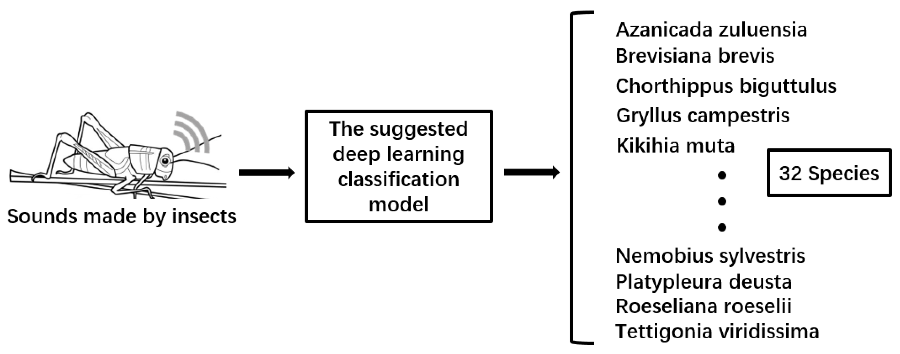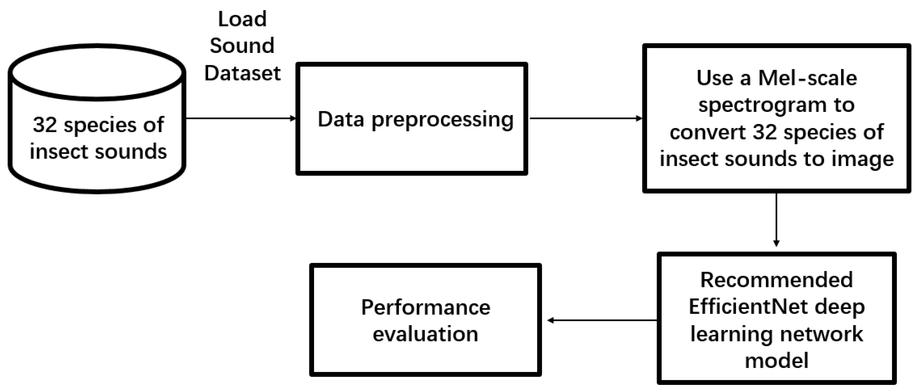In the field of deep learning, the general principles for processing insect sound classification are shown in Figure 1.

The proposed approach comprises three main components. The initial phase involves preprocessing insect sound data. The second phase employs the Mel-scale spectrogram method to convert raw audio data into an image format. The final phase encompasses feature extraction and classification using the dual-tower network. Insects’ sound clarity may offer vital insights into their species. Hence, this paper employs a series of signal processing techniques and feature extraction methods to acquire sound data that is more distinct and recognizable.

Figure 2 presents the process of the proposed deep-learning model for insect sound classification. Preprocessing, data augmentation, feature extraction, and classification all constitute integral elements of the proposed deep-learning model for insect sound classification. The proposed model consists of two primary steps: the first step entails feature extraction using EfficientNet [24], while the second step further enhances classification performance through the use of DFSM.

2.2.1. Data Preprocessing

Because insect sounds can vary significantly depending on factors [25] such as species, environment, behavior, and recording conditions, the limited number of available samples, and the fact that recordings are often affected by environmental noise, changes in recording equipment, and other sources of variation, data augmentation is necessary. Data augmentation of training models on the current dataset involves not only in-modeling but also generating carefully modified copies of new samples. These copies retain similar properties to the original data but are altered to make them appear to come from a different source or subject. This process is critical to ensuring that deep learning models can better handle the diversity of training data.

For audio data, all preprocessing is performed dynamically at runtime. We establish a transformation pipeline to read audio files through the respective library [26]. Within the dataset, monaural files are duplicated to the second channel, converting them to stereo, and standardizing the channel count for all audio files. Simultaneously, all audio is normalized and sampled at a rate of 44,100 Hz, ensuring uniform dimensions for all arrays. Audio duration is adjusted, either extended or shortened, through methods such as silent padding [27] or truncation [28] to match the length of other samples. This guarantees the elimination of feature differences between different audio files, providing uniform data for subsequent data augmentation and model training.

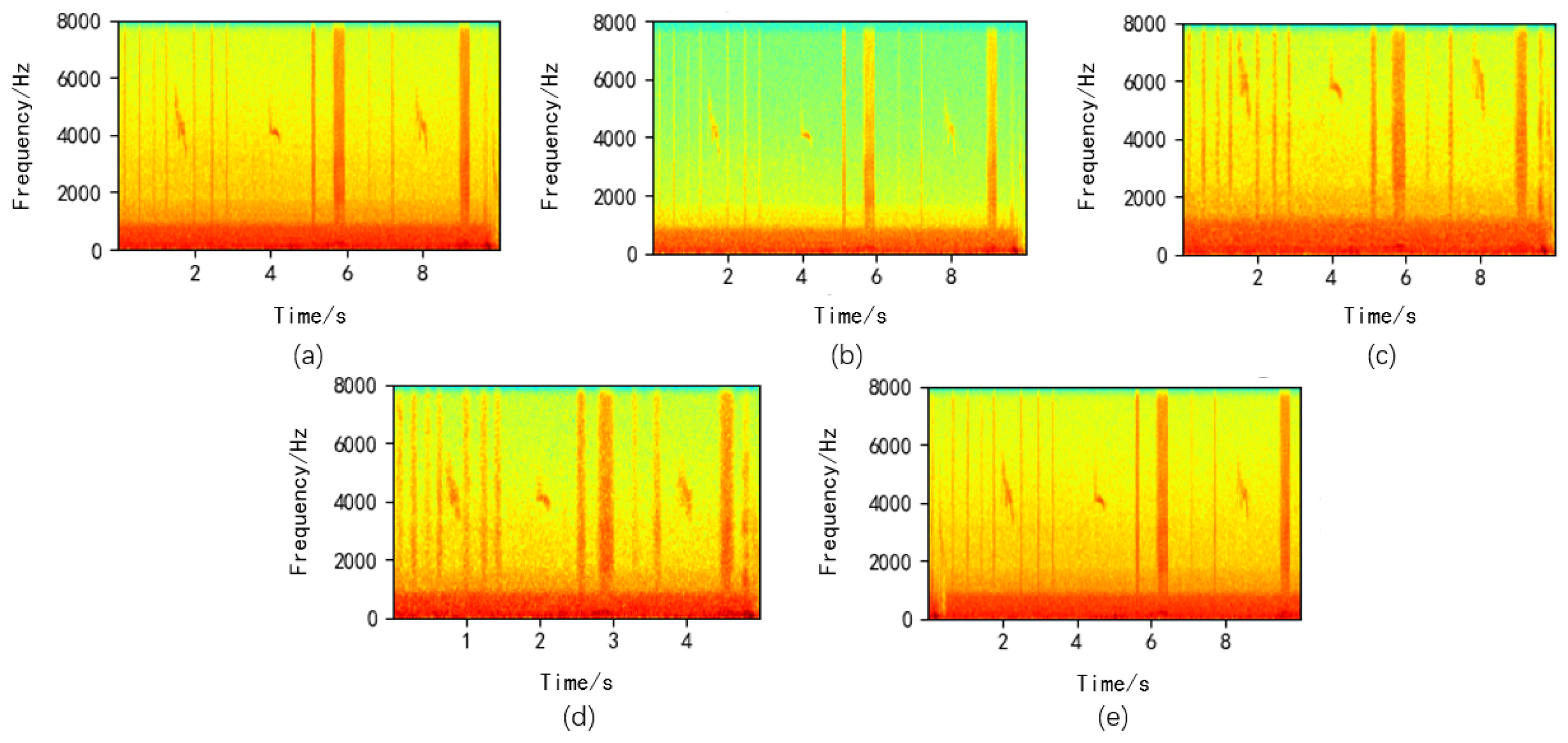
After data standardization, this paper augments insect sound data using noise addition [29], pitch shifting [30], time stretching [31], and time shifting [32], as shown in Figure 3. Noise addition entails introducing noise into the original audio signal to enhance the model’s adaptability to noise interference. Pitch shifting alters the signal’s pitch to improve the model’s recognition capabilities. Time stretching, achieved through temporal expansion, broadens the range of temporal variations in the training data, making the model more robust. Time shifting randomly displaces the audio signal to the left or right to augment the original audio data, increasing the diversity of the training data and enabling the model to better accommodate audio inputs at different speeds.

2.2.2. Mel-Scale Spectrogram

The perception of sound by the human ear is highly complex and nonlinear, particularly across different frequency ranges where distinct perceptual differences arise. However, insect sound signals often span a wide frequency range. In addition, human ear perception differs from a linear frequency scale. As frequency increases, human auditory sensitivity decreases, resulting in much smaller perceptual differences for high-frequency sounds compared to low-frequency sounds. To better simulate the auditory behavior of the human ear, we propose using the Mel scale [33], a nonlinear frequency scale. It converts the ordinary frequency (Hertz) f into the Mel frequency (Mel) m using Equation (1):

$$M\left(f\right)=2595·lg(1+\frac{f}{700})$$

(1)

Figure 3. Data Augmentation Diagram ((a): Original Image, (b): Noise Addition, (c): Pitch Shifting, (d): Time Stretching, (e): Time Shifting).

Figure 3. Data Augmentation Diagram ((a): Original Image, (b): Noise Addition, (c): Pitch Shifting, (d): Time Stretching, (e): Time Shifting).

To map spectral information to the Mel-scale frequency domain, we utilize a set of Mel filters [34]. These filters are evenly distributed on the Mel scale. The center frequencies of these Mel filters are configured according to the Mel scale to mimic the way the human ear perceives sound.

Creating the Mel spectrum entails convolving the spectral data obtained through the short-time fourier transform (STFT) [35] with the response of each Mel filter and computing the energy $E_i$ within each frequency band of the Mel filter. This step generates an energy value for each frequency band using Equation (2), resulting in the formation of the Mel spectrum. The STFT, on the other hand, transforms audio data from the time domain to the frequency domain. It decomposes the signal into frequency components within a series of time windows and conducts the transformation of audio data and spectral information as per Equation (3). Here, $X(t,f)$ represents the complex representation at time t and frequency f, $x\left(\tau \right)$ stands for the input audio signal, $\omega (\tau -t)$ corresponds to the window function, and $e^{-j2\pi ft}$ denotes the complex exponential term. Spectrograms, or Mel spectrograms, portray the signal’s strength over time at different frequencies by using a variety of colors for visual representation.

$$E_i=\sum _f{\left|X(t,f)\right|}^2$$

(2)

$$X(t,f)={\int }_{-\infty }^{\infty }x\left(\tau \right)·\omega (\tau -t)·e^{-j2\pi ft}d\tau$$

(3)

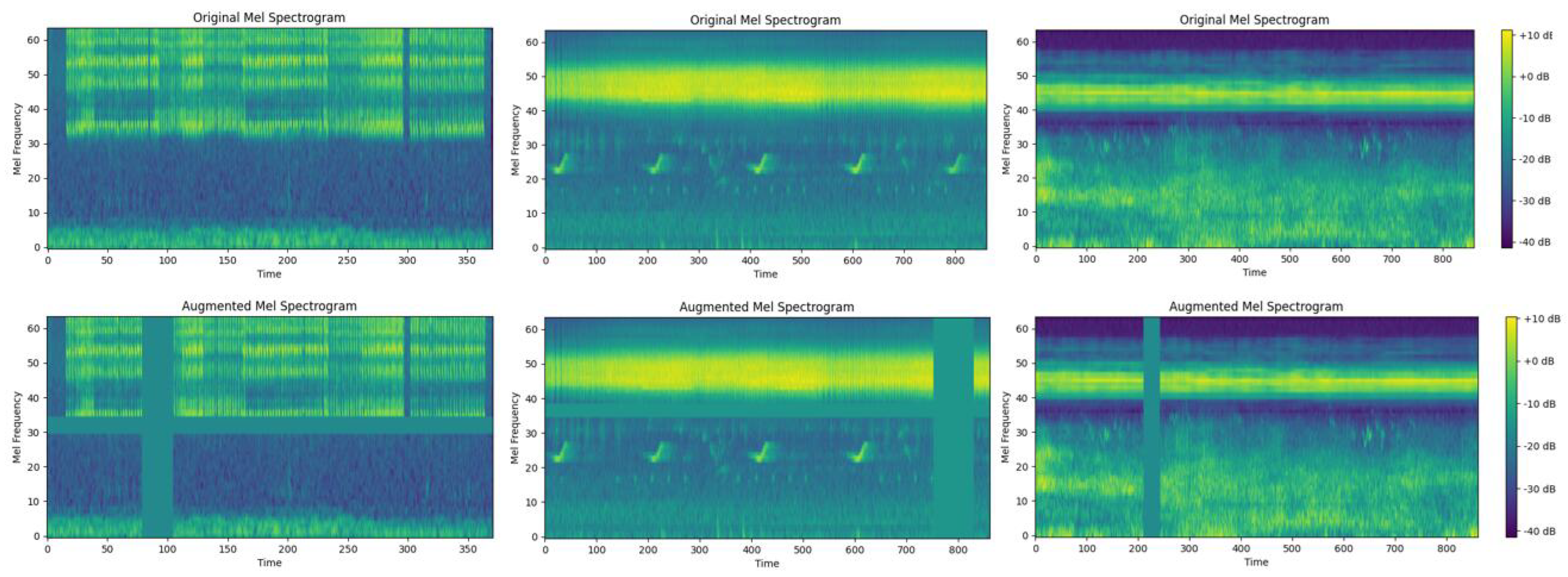
By applying a logarithmic transformation to the Mel spectrogram, we enhance the features and map them to a range more suitable for deep learning models, resulting in the logarithmic Mel spectrogram. This captures the fundamental characteristics of the audio. Building upon this, we apply the SpecAugment technique [36] to the logarithmic Mel spectrogram, as shown in Figure 4. Introducing horizontal bars via frequency masking and randomly masking time ranges by blocking vertical lines in the spectrogram. This is used to increase data diversity, simulate noise in different environments, or adjust the spectral characteristics of the signal, further enhancing data augmentation.

2.2.3. Deep Learning Framework

In the field of insect sound classification, a long-standing challenge has been how to accurately extract useful features from complex insect sound recordings for classification. To address this challenge, we conducted a study and introduced the dual-tower network, which comprises two main components: the EfficientNet-b7 module and the “dual-frequency and spectral fusion module (DFSM)”. In our research, we adopted the EfficientNet-b7 model as the foundational network. Its distinctive network architecture and parameter optimization techniques equip the EfficientNet model with superior feature learning capabilities, enabling it to capture intricate data features efficiently. The design concept of DFSM comes from how the insect brain processes sound signals and the mechanism of the insect auditory system. This module amalgamates some technical elements to achieve efficient audio feature classification. 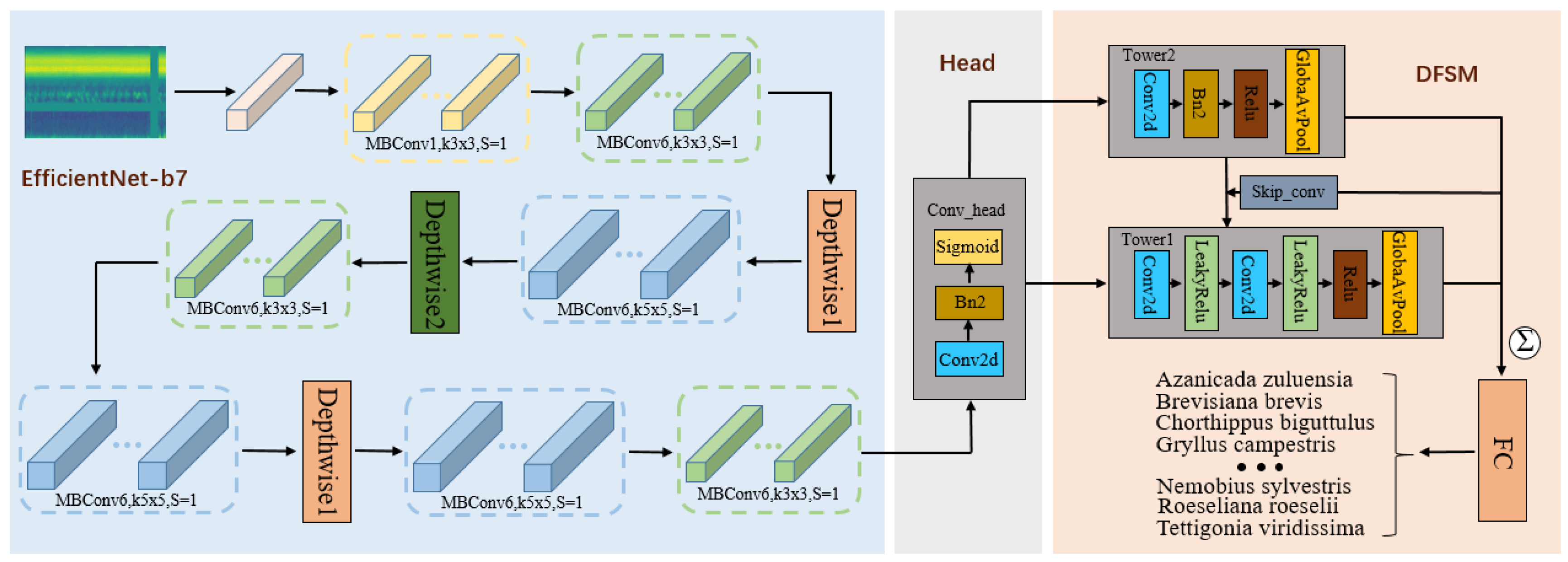By employing depthwise separable convolutions [37], the model becomes proficient at learning diverse frequency and temporal features. Additionally, the utilization of pooling operations aids in reducing data dimensions while preserving critical information. The incorporation of skip connections fosters interaction and integration among features at different levels, enabling the model to attain a thorough understanding of the complexity of audio signals. Through experimental comparisons with conventional methods, we have demonstrated that the DFSM can improve the accuracy of insect sound classification. The architectural layout of the dual-tower network is illustrated in Figure 5. This research not only introduces an innovative approach to insect sound classification but also imparts valuable insights into the principles of audio feature extraction, offering robust support for future studies in audio classification.

Unlike traditional image data processing, for audio transformation using Mel spectrograms, we consider the size in terms of the number of Mel frequency bands multiplied by the number of time steps as the input dimensions (as presented in

Table 2. Dual-Tower Network—Each row describes a stage ‘i’ with ‘$L_i$’ layers, input Mel frequency bands, time steps <$S_i,T_i$>, stride, and output channel count ‘$C_i$’.

Stage	Operator	Resolution	Channels	Layers	Stride
i	${\mathit{F}}_{\mathit{i}}$	${\mathit{S}}_{\mathit{i}}\mathbf{\times }{\mathit{T}}_{\mathit{i}}$	${\mathit{C}}_{\mathit{i}}$	${\mathit{L}}_{\mathit{i}}$
1	Conv3 × 3	64 × 344	64	1	2
2	MBConv1,k3 × 3	48 × 172	32	4	1
3	MBConv6,k3 × 3	48 × 172	48	7	1
4	MBConv6,k5 × 5	48 × 172	80	1	2
5	MBConv6,k5 × 5	24 × 86	80	6	1
6	MBConv6,k3 × 3	24 × 86	160	1	2
7	MBConv6,k3 × 3	12 × 43	160	9	1
8	MBConv6,k5 × 5	12 × 43	224	10	1
9	MBConv6,k5 × 5	12 × 43	384	1	2
10	MBConv6,k5 × 5	6 × 21.5	384	12	1
11	MBConv6,k3 × 3	6 × 21.5	640	4	1
12	Conv_head,k1 × 1	6 × 21.5	2560	1	1
13	Tower1,k3 × 3	1 × 1	2	1	1
14	Tower2,k1 × 1	1 × 1	2	1	1
15	Skip,k1 × 1	1 × 1	2	1	1
16	FC	1 × 1	32	1

). To better adapt to the input of Mel spectrograms, in ‘Stage 1’, we modify the number of channels to 2, and the output channel count is set to 64, while the remaining parts follow the original framework of EfficientNet-b7. We position the head module at the output layer of EfficientNet-b7, connecting it to the DFSM. In the first convolution layer of both tower1 and tower2, we set the output channel count to 2 and establish a skip connection, leaving the final FC layer with an “$in\_features$” value of 6. Furthermore, since the ‘$tower1\_pool$’ and ‘$tower2\_pool$’ methods employ ‘AdaptiveAvgPool2d’ for adaptive average pooling, the dimensions of the feature maps are reduced to 1 in length and width.

EfficientNet [24] represents a series of convolutional neural network models that rely on automated network scaling techniques. The distinctive feature of it is its network structure, which is determined through an automated search for the optimal configuration. This process involves a delicate balance between complexity and computational resources, as well as the scaling of different network layers. EfficientNet-b7, a deep and high-performance convolutional neural network, was chosen primarily to strike a balance between model depth, computational efficiency, and accuracy. While EfficientNet-b7 indeed delivers improved accuracy, it comes at the cost of an increased number of parameters compared to smaller variants in the EfficientNet series. This often necessitates a trade-off between performance, computational complexity, and model size.

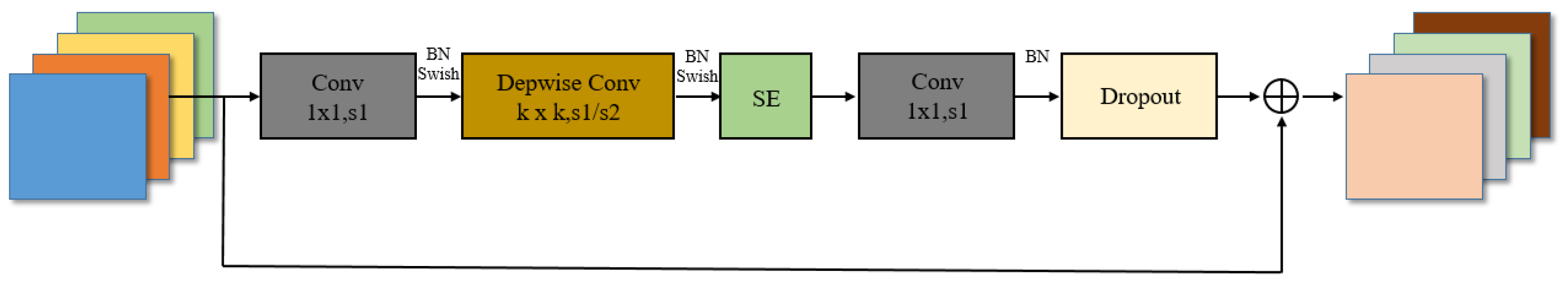
In the case of Mel spectrograms converted from insect sounds, we adapt the input channels of the model’s initial convolutional layer from 3 to 2 to accommodate audio Mel spectrogram input. The backbone network of EfficientNet-b7 is built by stacking MBConv structures, which comprise multiple recurrent convolutional blocks. Each convolutional block includes multiple convolution layers, batch normalization layers, and activation functions, as illustrated in Figure 6. MBConv1,6 represents the expansion factor of the output channels. Utilizing this deep architecture for extracting rich, high-level features proves instrumental in capturing complex information from insect sounds. These extracted features are subsequently fed into the DFSM for further processing and classification, enabling the network to comprehend more intricate image patterns.

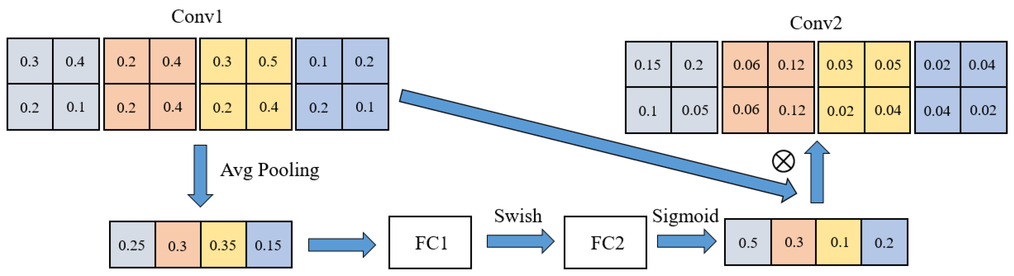
The squeeze-and-excitation (SE) module is an attention mechanism that comprises a global average pooling layer and two fully connected layers (as depicted in Figure 7). This module enhances the network’s focus on essential features, offering channel-wise adaptive weighting to feature maps, consequently improving the model’s expressiveness and performance. In the case of EfficientNet-B7, the SE module is applied to the output of each residual block [38] to heighten the network’s attention to critical features, thereby further enhancing the model’s accuracy.

In nature, insect sounds serve various purposes, from mating and warning to navigation. These sounds, produced by these diminutive organisms, serve as a medium of communication, yet they are also influenced by environmental noise and intricate acoustic characteristics. It’s in this context that the research team began contemplating whether inspiration could be derived from insect biology to improve the classification of insect sounds.

A comprehensive exploration of the auditory organs and systems of insects [39] revealed that they predominantly consist of auditory hairs, Johnston’s organs, and tympanic organs. These systems employ a hierarchical approach when processing sound. Insect brains [40] contain distinct groups of neurons, each responsible for processing different aspects of sound, such as frequency, temporal, and spectral characteristics. This allows insects to efficiently recognize sounds from companions or potential threats while filtering out noisy background sounds.

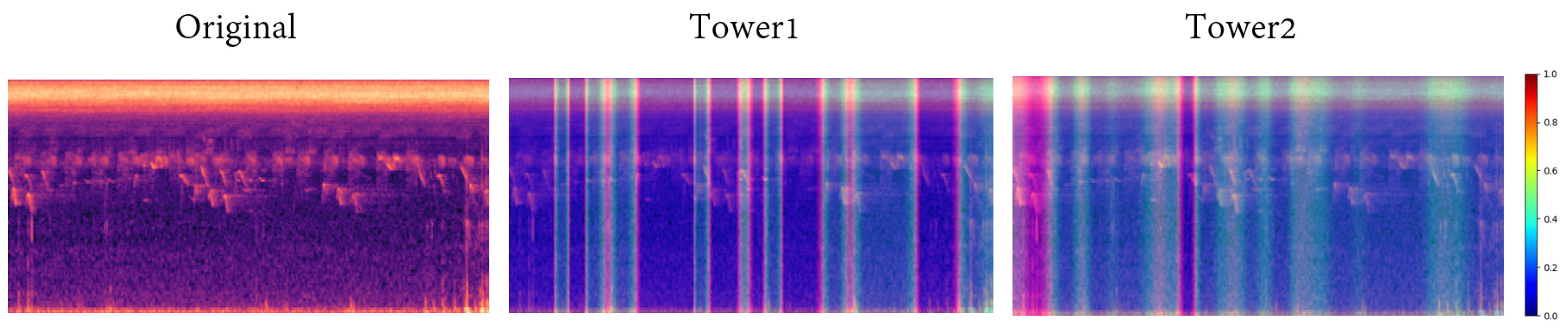
Taking inspiration from this hierarchical processing approach, we designed the DFSM. This module comprises two independent “towers”. Tower 1 consists of three convolutional layers, activation functions, and pooling layers, which function similarly to an insect’s temporal neuron group, focusing on capturing time features. It exhibits multiple dark features, enabling it to keenly discern various sounds. On the other hand, Tower 2 consists of one convolutional layer, an activation function, and a pooling layer; it emulates an insect’s spectral-perceiving neuron group, featuring only one or two dark areas in the CAM (class activation mapping) image [41]. It concentrates on capturing subtle differences in sound spectra (as shown in Figure 8), and spectral processing in insects effectively captures the hierarchical nature of insect sound perception. These two towers, along with their skip connections, enable the model to extract audio information from different perspectives, similar to insect neuron groups [39]. Furthermore, we designed a head module to connect EfficientNet and DFSM. The DFSM not only offers efficient feature extraction (hidden in the DNN(deep neural networks) layers and not accessible to the user) but also helps distinguish the time-frequency locations where subtle differences in insect sounds were extracted by the model. The design of this module draws inspiration from insect auditory systems, aiming to blend biology and deep learning to tackle the challenges of insect sound classification.

The dual-tower network, as proposed in this paper, standardizes insect sounds during the data preprocessing stage using a dual-channel configuration and a 44,100 Hz sampling rate. Furthermore, we introduce Gaussian noise with a standard deviation of 0.004 to enhance data diversity, ensuring experiment reproducibility with a specific random seed. To fine-tune the dual-tower network, we employ the Adam optimizer and conduct 400 epochs of training. During the training process, the batch size is set to 10, while the learning rate remains at 0.001. All experiments are carried out utilizing an NVIDIA RTX 3070 GPU (NVIDIA, Santa Clara, CA, USA) and an Intel server, thereby fully harnessing computational resources to ensure the stability and reliability of the experiments. These settings and configurations contribute to the good performance of our sound classification tasks. Specific experimental parameters are outlined in

Table 3. Specific Model Configuration Parameters.

Batch_Size	Lr	Channel	Noise	Pitch_Shift	Time_Shift	Sr	Mel
10	0.001	2	0.004	0.15	0.4	44,100	64

:

3. Results

We utilized an open-source dataset and employed Equation (1) to transform sampled insect sounds into Mel spectrograms for data processing. With the parameter settings described above, the model achieved an accuracy of 80.26%, showcasing its proficiency in distinguishing between sounds produced by different insect species.

When assessing the model’s performance, we partitioned the dataset into training, and test sets, aligning them with the official CSV files where each class corresponds to a unique $class\_id$ (as detailed in

Table 4. Mapping of Species to $Class\_id\left(Cid\right)$.

Species	Cid	Species	Cid	Species	Cid	Species	Cid
Azanicada zuluensis	0	Myopsalta mackinlayi	8	Platypleura chalybaea	16	Platypleura sp10	24
Brevisiana brevis	1	Myopsalta melanobasis	9	Platypleura deusta	17	Platypleura sp11cfhirtipennis	25
Chorthippus biguttulus	2	Myopsalta xerograsidia	10	Platypleura divisa	18	Platypleura sp12cfhirtipennis	26
Chorthippus brunneus	3	Nemobius sylvestris	11	Platypleura haglundi	19	Platypleura sp13	27
Gryllus campestris	4	Oecanthus pellucens	12	Platypleura hirtipennis	20	Pseudochorthippus parallelus	28
Kikihia muta	5	Pholidoptera griseoaptera	13	Platypleura intercapedinis	21	Pycna semiclara	29
Myopsalta leona	6	Platypleura capensis	14	Platypleura plumosa	22	Roeseliana roeselii	30
Myopsalta longicauda	7	Platypleura cfcatenata	15	Platypleura sp04	23	Tettigonia viridissima	31

). The confusion matrix showing the performance of the dual-tower network reflects the overall performance as it shows a clearer diagonal for accurate classification. During our analysis, we identified specific trends and patterns of misclassification. Notably, a large portion of misclassifications occurred within the genera Myopsalta and Platypleura from the InsectSet32 dataset, encompassing 5 and 14 distinct species, respectively (illustrated in Figure 9). It is worth mentioning that species within these genera were frequently mislabeled as other members of the same genera. Within its genus, we observed that one insect species called M. melanobasis(9) caused a significant number of misclassifications, and the model has a lot of confusion in this category. Similarly, 14 species within the Platypleura genus, including P. capensis(14) and P. divisa(18), were often incorrectly categorized as other members within the same genus. Brevisiana brevis(1) and Pholidoptera griseoaptera(13) were never correctly classified. Compared with other network models, the model performance of the dual-tower network is significantly better for insect sound recognition.

4. Discussion

The learning rate is a hyperparameter used to update weights during the gradient descent process. In this regard, we conducted a comparative experiment to determine the optimal initial learning rate, as presented in

Table 5. Performance Comparison of Different Learning Rates.

Learning-Rate	Batch_Size	Accuracy	F1	Recall	Precision
(${\mathbf{10}}^{\mathbf{-}\mathbf{3}}$)		(%)	(%)	(%)	(%)
0.3	10	75.00	65.46	66.04	71.46
0.6	10	75.00	59.81	62.55	62.24
0.9	10	78.95	56.04	58.49	60.56
1	10	80.26	62.02	65.68	65.66
3	10	72.37	60.73	63.85	64.69
6	10	68.42	47.52	52.81	46.93
9	10	68.42	44.80	47.97	48.01

.

The feature extraction module is employed to reduce the dimensionality of certain raw input data or restructure the original features for subsequent use. Its primary function is to decrease data dimensionality and arrange existing data features. We compared the feature extraction module we utilized with several other classical feature extraction modules, and the results of different feature extraction modules are presented in

Table 6. Results (% for Accuracy, F1, and Recall) for Different Feature Extraction Modules. The best, second-best, and third-best results are highlighted in red, blue, and green, respectively.

Model	Accuracy	F1	Recall	Precision	Param	FLOPS
	(%)	(%)	(%)	(%)	(million)	(GigaFLOPs)
Resnet [42]+DFSM	67.11	47.63	49.74	52.12	23.54	1.82
Vgg16 [43]+DFSM	60.53	44.98	50.78	46.12	138.42	6.83
Vit [44]+DFSM	60.53	43.37	45.62	45.33	85.82	16.86
Efficientnet-b0 [24]+DFSM	76.32	56.64	59.48	60.46	5.31	0.02
Efficientnet-b1 [24]+DFSM	77.63	58.24	60.57	64.31	7.81	0.02
Efficientnet-b2 [24]+DFSM	75.00	55.66	58.65	56.82	9.13	0.02
Efficientnet-b3 [24]+DFSM	76.32	63.73	66.04	68.12	12.26	0.03
Efficientnet-b4 [24]+DFSM	73.68	60.89	66.06	64.07	19.37	0.03
Efficientnet-b5 [24]+DFSM	78.95	60.90	63.70	61.23	30.42	0.05
Efficientnet-b6 [24]+DFSM	77.63	57.42	60.21	59.93	43.08	0.06
Efficientnet-b7 [24]+DFSM	80.26	62.02	65.68	65.66	66.39	0.08

. The recall is only 0.38% away from the best performance, surpassing the second-best performance on this dataset by 0.36%. However, our model did not perform well in terms of precision, with a 2.5% difference from the best precision. The main reason is the potential similarity between categories of insects, rendering their sound features more challenging to distinguish. Additionally, as a feature extractor, EfficientNet has fewer parameters than other feature networks, and b7 outperforms b0-b6, making it better suited for capturing local features in insect sound data.

In this study, we conducted a performance comparison of various models, including ResNet50 [42], RegNet [45], ConvNext [46], MnasNet [47], ShuffleNetV2 [48], MLP-Mixer [49], DenseNet201 [50], MobileNetV2 [51], Swin transformer [52], and our dual-tower network (as presented in

Table 7. Performance Comparison of Different Models.

Model	Accuracy	F1	Recall	Precision	Param	FLOPS
	(%)	(%)	(%)	(%)	(Million)	(GigaFLOPs)
ResNet50 [42]	63.16	43.73	47.19	43.97	25.58	1.82
RegNet [45]	73.68	52.30	58.80	52.27	107.84	14.15
ConvNext [46]	59.21	46.44	51.51	45.89	4.65	0.79
MnasNet [47]	52.63	40.27	44.06	44.30	5.28	0.15
ShuffleNetv2 [48]	73.68	52.36	55.78	54.08	2.31	0.07
MLP-Mixer [49]	61.84	42.63	46.72	46.51	17.90	3.76
DenseNet201 [50]	61.84	44.49	48.28	47.60	21.23	0.11
MobileNetv2 [51]	78.95	57.20	59.01	59.05	3.54	0.14
Swin Transformer [52]	63.16	50.34	51.87	54.36	27.54	4.37
Dual-Tower Network	80.26	62.02	65.68	65.66	66.39	0.08

) and visualized the results using bar charts (as illustrated in Figure 10). During the training of the MLP-Mixer [49] and Swin transformer [52] models, the Mel spectrogram input for insect sound conversion was [10, 2, 64, 344], while the model expected input in the shape of [10, 2, 224, 224]. To address this, we applied array sampling operations using a bilinear sampling algorithm with the “$alig{n}_{c}orners$” set to false. This ensured that input and output tensors were aligned at their corner pixels (as demonstrated in Figure 11). For out-of-bounds values, interpolation using edge values was employed, allowing for a scientific adjustment of the array dimensions while preserving data integrity. The remaining comparative experiments involved deep learning transfer models.

To gain a deeper understanding of the performance of the dual-tower network and the contributions of its components, we conducted a series of ablation experiments. In these experiments, we progressively removed different parts of the DFSM, including the DFSM itself and the two separate tower structures. Based on the experimental data presented in

Table 8. Comparative Results of Ablation Experiments.

Model	Accuracy	F1	Recall	Precision	Param	FLOPS
	(%)	(%)	(%)	(%)	(Million)	(GigaFLOPs)
EfficientNet-b7	75.00	60.05	62.45	60.94	25.58	1.82
EfficientNet-b7+T1	76.32	57.45	62.34	63.12	55.26	0.98
EfficientNet-b7+T2	76.32	61.82	64.48	64.69	36.71	0.79
EfficientNet-b7+T1+T2	80.26	62.02	65.68	65.66	66.39	0.08

, we observed that removing the DFSM decreased the model’s performance, resulting in a 5.26% decrease in accuracy (as shown in Table 2). All other metrics (F1, Recall, and Precision) also showed declines. This strongly indicates the substantial contribution of the DFSM to the task. Building on this discovery, we removed Tower 1 and Tower 2 to validate the importance of each tower further, both of which led to decreased model performance.

When conducting generalization experiments, our focus is on verifying the performance of the dual-tower network on different datasets and its ability to generalize in practical applications. This paper selected three diverse datasets, including environmental sounds from ESC-50 [17], urban sounds from UrbanSound8K [18], and speech commands from Speech Commands [19]. Each dataset represents distinct sound backgrounds and classification tasks. This experimental design enables a comprehensive evaluation of the model’s adaptability and generalizability, providing insights into its performance across various sound environments.

Through a series of steps involving data preparation, model application, and performance evaluation, we achieved good results, as presented in

Table 9. Model Comparison on Different Datasets.

Dataset	Methods				Dual-Tower Network
	Model	Acc (%)	Model	Acc (%)	Acc (%)	F1 (%)	Rec (%)	Pre (%)
ESC-50 [17]	ACDNet [53]	87.10	AVID [54]	89.20	85.75	80.07	80.25	82.16
UrbanSound8K [18]	FACE [55]	98.05	PIPMN [56]	96.00	97.89	97.04	97.10	97.00
Speech Commands [19]	Q-CNN [57]	95.12	TDNN [58]	94.30	93.94	93.87	93.87	93.99

. The dual-tower network attained an accuracy of 85.75% on the ESC-50 dataset, showcasing its capacity to recognize diverse sound categories in a natural environment and underscoring its potential to adapt to natural sound backgrounds. It demonstrated good performance on the UrbanSound8K dataset, achieving an accuracy of 97.89%, which is particularly true given the complex conditions of urban environments, including urban noise and various sound events. Furthermore, the model exhibited success on the Speech Commands dataset, with an accuracy of 93.94%, further confirming its practicality in speech command recognition and speech-to-text tasks. The outcomes of this series of experiments underscore the superior performance. Its effectiveness extends beyond insect sound classification tasks to behave well in various soundscapes and tasks, making it a valuable asset for practical applications across multiple domains.

5. Conclusions

The dual-tower network proposed in this paper demonstrates great performance and wide applicability in insect sound classification tasks. Using the method we propose, an accuracy of up to 80.26% can be achieved. Furthermore, we validated the proposed method on other datasets and compared it with alternative approaches. Experimental results confirm that the dual-tower network exhibits great performance across diverse datasets with minimal data-specific impact, showcasing strong generalization capabilities. This indicates that utilizing deep learning networks to emulate biological communication can effectively enhance feature extraction and predictive accuracy. Our research provides valuable insights for pest monitoring and biological control technologies, offering an empirical foundation for future research endeavors.

Considering future research directions, we fully appreciate the opportunities to contribute to the field, building upon the work of previous scholars. We firmly believe that there is ample room for exploration in the current research. The future work will focus on expanding multimodal research, with a deeper emphasis on integrating multimodal data with biological theories and ecological concepts. We aim to explore how to extract more ecological and behavioral information from audio and visual signals, facilitating a better understanding of animal behaviors and ecosystem interactions.