Improved Convolutional Neural Network–Time-Delay Neural Network Structure with Repeated Feature Fusions for Speaker Verification

Abstract

The development of deep learning greatly promotes the progress of speaker verification (SV). Studies show that both convolutional neural networks (CNNs) and dilated time-delay neural networks (TDNNs) achieve advanced performance in text-independent SV, due to their ability to sufficiently extract the local feature and the temporal contextual information, respectively. Also, the combination of the above two has achieved better results. However, we found a serious gridding effect when we apply the 1D-Res2Net-based dilated TDNN proposed in ECAPA-TDNN for SV, which indicates discontinuity and local information losses of frame-level features. To achieve high-resolution process for speaker embedding, we improve the CNN–TDNN structure with proposed repeated multi-scale feature fusions. Through the proposed structure, we can effectively improve the channel utilization of TDNN and achieve higher performance under the same TDNN channel. And, unlike previous studies that have all converted CNN features to TDNN features directly, we also studied the latent space transformation between CNN and TDNN to achieve efficient conversion. Our best method obtains 0.72 EER and 0.0672 MinDCF on VoxCeleb-O test set, and the proposed method performs better in cross-domain SV without additional parameters and computational complexity.

1. Introduction

Speaker verification (SV) refers to the method of confirming the identity of a speaker through the speaker’s personal information in speech signals. SV has been widely used in various fields, such as speaker diarization, speech enhancement [1], and voice conversion [2]. In recent years, the research on SV algorithms based on deep learning has made great progress. In general, the procedure of the SV task falls into two steps. First, the embeddings of speaker utterances are extracted through deep neural networks, such as X-Vector systems [3,4,5]. Then, the similarity scores between the registered enroll–test pairs are calculated by normalized cosine similarity methods [6,7,8,9], PLDA [10], or other back-ends [11,12]. A series of speaker encoders are mainly trained by the famous angular softmax loss functions, including AM-softmax [13] and AAM-softmax [14], which are highly effective. Some studies have also published the efficient end-to-end triplet loss [15] or contrastive loss [16,17] for SV.

Today, the most efficient SV methods are TDNN and their variant networks. TDNN is generally considered a method that can fully extract the long temporal information of the input acoustic signal [18]. And ECAPA-TDNN [19], proposed in 2020, has achieved state-of-the-art performance on the large-scale voiceprint recognition dataset Voxceleb [20,21] by introducing the TDNN-based model with dilated convolution, propagation, and aggregation strategies. In addition, studies [22,23,24] show that CNNs are very suitable for processing the speech spectrogram, which can fully perceive and extract the texture information in different receptive fields. The ResNet backbone network, for example, can build a lightweight, stable, and robust speaker recognition model [23,25].

Naturally, a combination of the above two achieves better results [24,26,27,28]. In the CNN–TDNN structure, a CNN front-end is added before TDNN to extract enough local information of the input spectrogram. The features are then sent to TDNN blocks to calculate the temporal contextual features. The CNN–TDNN framework is undoubtedly effective, but it always leads to a larger model size and higher calculational load. Motivated by [29], we believe there is still plenty of scope for improvement by introducing high-resolution fusions.

Furthermore, residually dilated TDNN networks lead to advanced performance in SV [26,27,30] due to their excellent performance in capturing temporal contextual information. The utilization of dilated convolution extends the receptive field of the TDNN layers, enabling dense feature representation without introducing any additional parameters [19], thereby extracting features in a fully temporal resolution until global embedding and achieving high-resolution feature extraction. Compared with the pooling strategy, it also avoids the loss of temporal-frequency information and maintains the resolution of feature maps [31]. However, we find that the discontinuous sampling of dilated TDNN introduces a serious gridding effect [32,33], which will result in information loss and a decline in the quality of acoustic frame-level features.

In this letter, we propose a CNN–TDNN architecture with repeated fusions for SV, and the framework is exhibited in Figure 1. Our contributions mainly include the following four aspects: (1) we propose a competitive structure without additional number of parameters for high-resolution speaker embedding, which means better performance in SV; (2) we search for CNN encoders with temporal-frequency bottlenecks to extract multi-scale features in the time dimension; (3) we study the structures of repeated multi-scale feature fusions (RMSFs) to ensure the high-resolution feature extraction of TDNNs; and (4) we train the parameter weights using English datasets and test them on the CN-Celeb set. The results indicate that our method presents surprise improvement in cross-domain adaption SV tasks.

2. Proposed Method

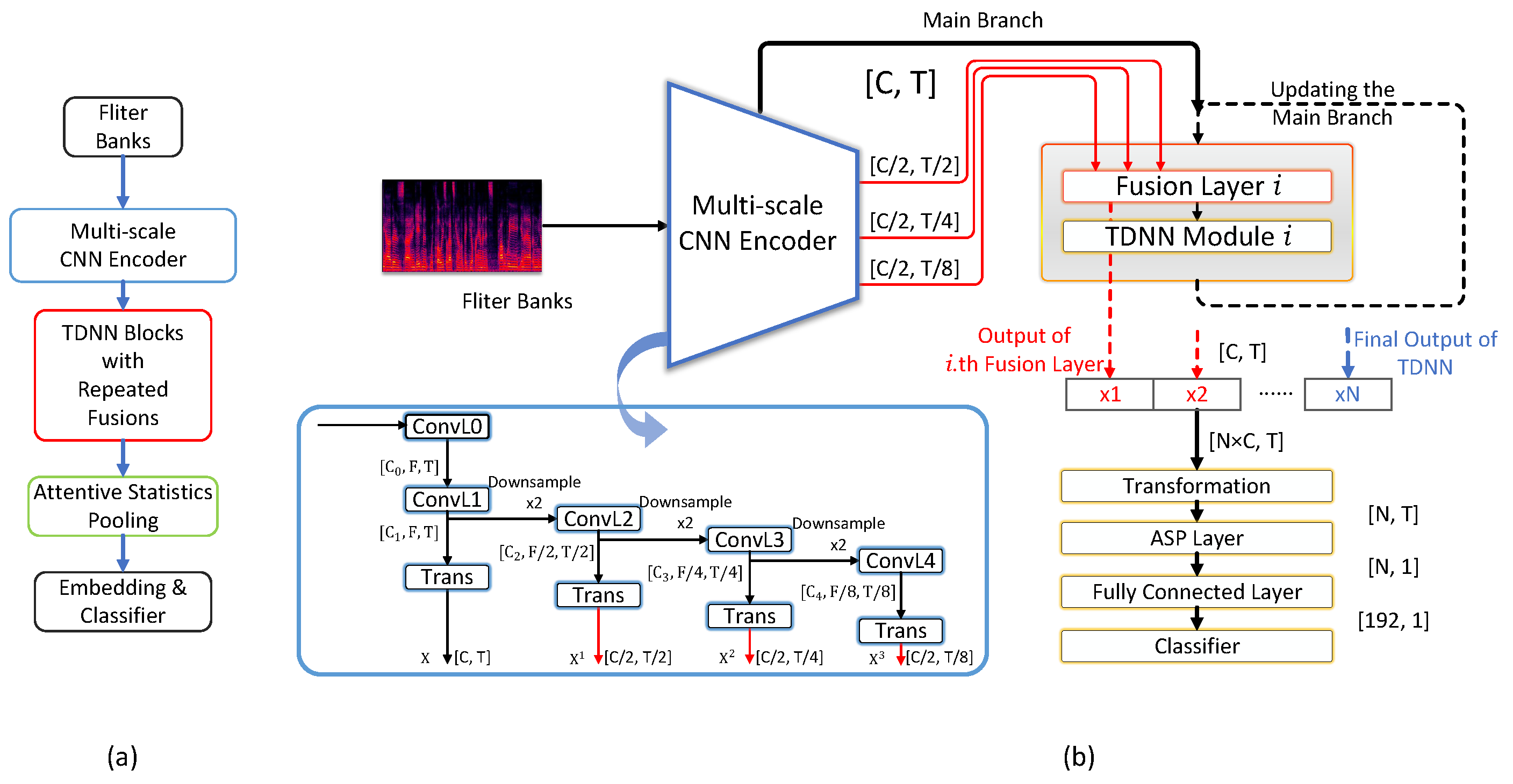
2.1. CNN Encoder for Multi-Scale Features

2.1.1. CNN Backbone

In the SV task, it is often crucial to extract key point signals that are conducive to speaker representation. To achieve high-resolution representation for speakers, making full use of multi-scale feature representation is considered effective. Thus, we employ a deep CNN encoder to obtain temporal-frequency features at different scales.

We exploit the popular residual network backbone [25] to obtain features of different scales at different depths, which will then be reshaped to 2D matrices through the proposed bottleneck transformation layers. And in our research, we found that the number of residual units in each convolution layer should be kept at three or more, to extract sufficiently good feature maps, but large channels are unnecessary. We also add SE module [35] for each unit of the residual network to calculate the attention of channels, which is widely considered effective for highlighting important local frequency regions.

Supposing that the input frame-level filter banks feature of CNN encoder is $X_{sepc}\in R^{F\times T}$. Four branches are obtained with different downsample rate in total. We call the branch without downsampling as the main branch, and other branches are minor branches marked by red in color as shown in Figure 1b. And, we found that $C=512$ is enough for a effective SV task in our network structure.

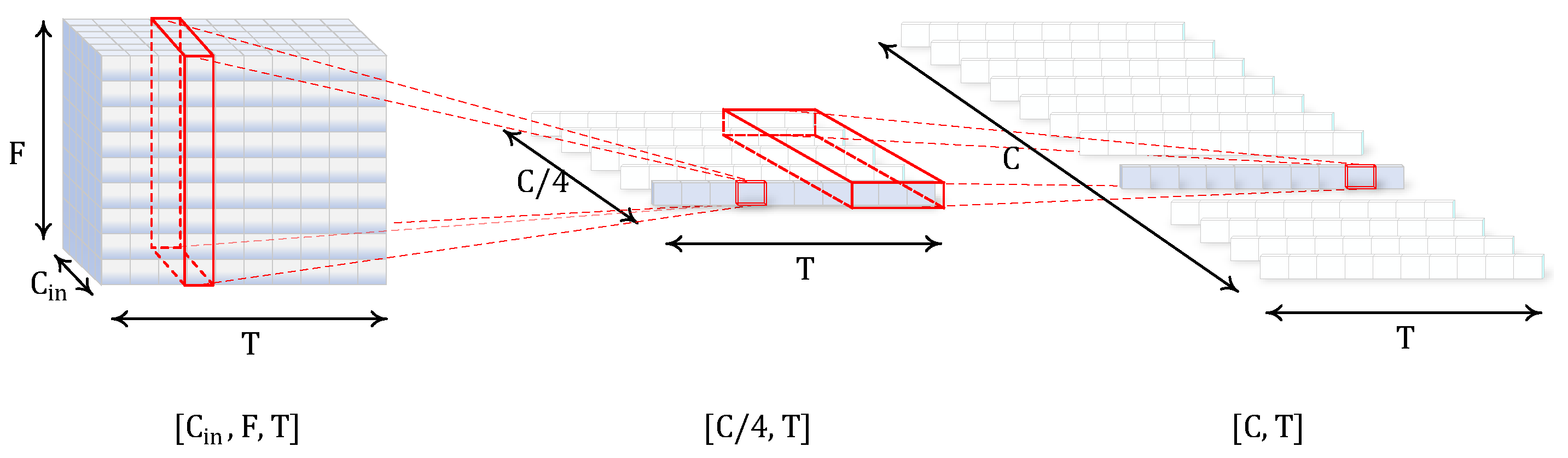
2.1.2. Bottleneck Transformation

In our preliminary experiments, it was found that utilizing a direct feature transformation between CNNs and TDNNs results in inferior performance. We consider that is because the CNN encoder and TDNNs have different latent spaces of features. To obtain frame-level feature maps matching the input of the following TDNN blocks, we propose the bottleneck transformation structure located at the junction of CNNs and TDNN blocks. The feature maps of each branch from the CNN encoder are first flattened, then expanded through the transformation. As is shown in Figure 2, for each branch with a shape of $R^{C_{in}\times F\times T}$, the transformation is expressed as:

$$\begin{array}{cc}\hfill & M=Concat[M_1,M_2,\dots ,M_{C_{in}}]\hfill \\ \hfill & X_{neck}=BN\left\{ReLU\left[Conv1d{|}_{k=1}\left(M\right)\right]\right\}\hfill \\ \hfill & X=BN\left\{ReLU\left[Conv1d{|}_{k=3}\left(X_{neck}\right)\right]\right\}\hfill \end{array}$$

(1)

where $M_i\in R^{F\times T}$ indicates the feature map of channel i and $M\in R^{[C_{in}\times F]\times T}$ represents the reshaped 2D matrix. ‘BN’ means batchnorm. The channels are firstly squeezed to $C_{out}/4$ and obtain $X_{neck}\in R^{C_{out}/4\times T}$, then we extend the feature map to $X\in R^{C_{out}\times T}$. The transformation layer compresses the feature maps, which is beneficial to more major information with less computation. We suppose that $X\in R^{C\times T}$ is the output of main branch, and $X^i\in R^{C/2\times T/2^i}$ refers to output of the ith minor branch with a downsample factor of $2^i$ in time dimension, $i=\{1,2,3\}$. The shape of X is maintained through all the TDNN blocks to ensure a high-resolution expression, while minor branches are applied to fuse with the main branch repeatedly in every TDNN block.

2.2. TDNN Blocks with Multiple Fusion Layers

The Res2Net [36] module gets multi-scale frame-level features by enhancing the middle layer of the bottleneck block. However, we notice that serious gridding effect [32] emerged and the neighboring information is not fully taken into account when introducing constant dilation rate in 1D-Res2Net, as shown in Figure 3. Assume that the input feature $X\in R^{C\times T}$ is split into s feature map subsets, and the sth feature map $X_s$ can be expressed as: $X_s=\{x\left[1\right],x\left[2\right]\dots ,x\left[T\right]\}\in R^{C/s\times T}$.

For the sake of convenience, $C/s$ is defined as 1, which means we assume $X_s$ to be a single-channel. Consequently, the dilated convolution can be mathematically represented by the subsequent formula:

$$\begin{array}{c}\hfill y\left[i\right]=\sum _{l}x[i+r·l]·w^l\end{array}$$

(2)

where $x\left[i\right]$ and $y\left[i\right]$ denote the input and output signal, respectively. w is the filter with a filter length of 3, and $l=\{-1,0,1\}$. r means the dilation rate. Dilated convolutions return to standard convolutions when $r=1$.

So, for group convolutions in cascade, like Figure 3 shows, we can obtain:

$$\begin{array}{cc}\hfill y_n\left[i\right]& =\sum _l(x_n+y_{n-1})[i+r·l]·w_n^l,n⩾3\hfill \end{array}$$

(3)

Thus, taking $y_4$ as an example, where $w_k$ means the weight of TDNN_k in Figure 3a, we can intuitively deduce that:

$$\begin{array}{cc}\hfill y_4\left[i\right]=& \sum _l\sum _{l^{\prime }}\sum _{l^{\prime \prime }}{x}_2[i+r·(l+l^{\prime }+l^{\prime \prime })]·w_1^l{w}_2^{l^{\prime }}{w}_3^{l^{\prime \prime }}\hfill \\ & +\sum _{l^{\prime }}\sum _{l^{\prime \prime }}{x}_3[i+r·(l^{\prime }+l^{\prime \prime })]·w_2^{l^{\prime }}{w}_3^{l^{\prime \prime }}\hfill \\ & +\sum _l{x}_4[i+r·l]·w_3^l\hfill \end{array}$$

(4)

Although the receptive field of $y_4$ is extended to $2mr+1$, the actual receptive field is from isolated frames $\{i,i\pm r,i\pm 2r,i\pm 3r\}$. Frankly, there is no correlation for neighboring frames when $r>1$, and the accumulation between different TDNN blocks may cause a larger grid effect, which can result in information loss. The CNN–TDNN framework can be attributed to the CNN’s ability to better handle local feature information. However, the research above has shown that the dilated TDNN structure suffers from information loss due to the grid effect during computation. Moreover, the existing CNN–TDNN structure only reinforces local features at the input end of TDNNs, resulting in progressive information loss during the computation process of the TDNN backbone.

To address the information loss problem, and inspired by HRNet [29] to obtain high-quality features, a combination of repeated multi-scale fusions and dilated TDNN is introduced to compensate the TDNN blocks as demonstrated in Figure 4a. A fusion operator can be formulated as:

$$X_{fusion}=ReLU\{X+\sum _{i=1}^3{f}_i\left[B{N}_i\left(Conv1d{|}_{k=1}\left(X^i\right)\right)\right]\}$$

(5)

with $f_i[·]$ denoting upsample function with a scale factor of $2^{i-1}$, and we simply employ the simplest nearest neighbor interpolation for upsampling. ’BN’ means batchnorm. Therefore, the minor branches are extended to the same shape as the main branch to implement the multi-scale fusion. This enables each TDNN block’s computation to receive multi-scale information from the CNN encoder repeatedly, with information upsampled from different scales to enhance the relatedness of local neighbor features in time dimension. All of the features with strong correlation upsampled from minor branches will be fused with the main branch to fulfill the compensation of dilated TDNN blocks.

To exploit more information from different TDNN blocks, multi-layer feature aggregation (MFA) and residual summation connections [19] are adopted. The input of each TDNN block will be connected with the previous corresponding position by an element-wise addition, as is shown in Figure 4b. Especially for MFA, we made some adjustments to match the RMSFs. We aggregate the final TDNN block with all previous fusion layers except the first, just like Figure 1b depicted.

3. Experiments

3.1. Dataset

We conduct our experiment on the famous large-scale corpora-Voxceleb1&2 dataset [20,21]. For the training dataset, we use the Voxceleb2 development set, consisting of 1,092,009 utterances across 5994 speakers, and a small subset of it is reserved for validation. After training, the network is evaluated on different test subsets of Voxceleb1: VoxCeleb1-O (Vox1-O) and VoxCeleb1-H (Vox1-H). To prove the benefits of our proposed method for complex verification tasks, we directly conduct tests on different target domain set: CNCeleb1 test set [37]. We also fine-tuned the pre-trained models in the SV dataset:CNCeleb1&2 [37,38].

It should be noted that no CNCeleb subsets overlap with the Voxceleb2 development set, and we just utilize the original utterances for training or evaluating without the employment of voice activity detection.

3.2. Preprocessing and Data Augmentation

All audios are randomly cropped to 2 s in training, audios shorter than 2 s will be duplicated and concatenated to create a 2 s segment. And, the sampling rate is 16,000 Hz. Pre-emphasis with a coefficient of 0.97 is first applied. Then, 80-dimensional log Mel-filterbanks are extracted with a 25 ms hamming windows and 10 ms shift. The frequency is limited to 20–7600 Hz in Mel spectragrom. Since the downsampling requirements in the CNN encoder, the number of frames is cut into an integer multiple of 8. In addition, mean normalization in time dimension is applied.

Training audios are randomly augmented for a robust model. Our augmentation methods are mainly in terms of MUSAN dataset [39] and RIR dataset [40]. MUSAN provides three types of additional noise that can be mixed with the original sounds to generate augmented data. RIR has a variety of simulated room impulse responses for reverberation augmentation, which enhances the robustness of SV systems against various environmental interferences encountered during recording. In addition, we apply SpecAugment [41] in the pre-training stage, with random time masking and frequency masking, respectively, for all spectrograms. Considering the computational cost, no speed perturbation [42] is adopted in our experiments.

3.3. Baseline Systems and Experimental Details

3.3.1. Baseline Systems

Considering the outstanding performance of both the CNN framework with ResNet as the backbone and the TDNN network in SV, we reproduce the prevailing SE-ResNet [23], ECAPA-TDNN [19], MFA-TDNN [27] and ECAPA-CNN–TDNN [26] as our baseline systems.

In our research, some of the models are adjusted to a proper size and all baseline systems are trained or evaluated under the same conditions for a fair comparison, due to differences between the fine-tuning strategies and the hyperparameters used in different systems. All the parameters are displayed in our experiments. For MFA-TDNN, we reproduced the MFA-TDNN and adjusted it to a larger size. All other model reproductions primarily conform to the original references, while incorporating minor modifications as needed in our comparative experiments.

3.3.2. Training Strategies and Fine-Tuning Details

Trainable parameters are first optimized by Adam within 120 epochs, with initial learning rate of 0.001 as well as a decay factor of 0.97. The batch size is fixed to 512 for all training tasks. We apply AAM-softmax loss function [14] for all experiments. The margin and scale of AAM-softmax are set as 0.2 and 30, respectively. Then, we fine-tune [43] the pre-trained models over the following 10 epochs.

• Large-margin fine-tune:
  The large-margin fine-tune strategy is applied to the pre-trained models on the VoxCeleb dataset. In the fine-tune stage, we reset the batch size to 64. All input utterances are cropped to 6 s, and the margin of AAM-softmax is adjusted to 0.5. The initial learning rate is 2 × ${10}^{-5}$ with a decay rate of 0.9. SpecAugmentation is disabled, and the other settings remain unchanged.
• Cross-language fine-tune:
  In addition, we fine-tune the above pre-training models on the cross-language CN-Celeb1&2 dataset [37,38] to compare the cross language SV performance between the models. Taking into account the distribution of duration within the CNCeleb dataset, we made slight adjustments to the training parameters. We crop utterance into 4 s intervals for fine-tuning. The initial learning rate is reset to 1 × ${10}^{-5}$ with a decay rate of 0.9. While keeping other settings the same above.

3.3.3. Evaluation Protocol

After training, we extract 192-dimension speaker embeddings in test pairs and calculate the cosine similarity between embeddings of each pair, then adaptive s-norm [9] is performed with an imposter cohort size of 600. We measure the systems according to equal error rate (EER) and minimum of the normalized detection cost function (MinDCF). The EER represents the point at which the false acceptance rate and false rejection rate are equal. The MinDCF, which incorporates weighting for acceptance and rejection errors, is expressed as: $C_{det}=C_{miss}\times P_{\mathrm{miss}}\times P_{\mathrm{tar}}+C_{fa}\times P_{fa}\times \left(1-P_{\mathrm{tar}}\right)$. In our research, we consider a prior target probability $P_{target}$ of 0.01 and misses $C_{miss=}$ = false alarms $C_{fa}=1$.

4. Results

4.1. Comparison of Systems

In this section, we verify the performance of our proposed model by comparing with different advanced methods, and all results are displayed in

Table 1. The performance comparison by EER and MinDCF of produced networks and other SOTA models. All models are trained on the VoxCeleb2 dataset.

Model	Parms	Macs	VoxCeleb1-O		VoxCeleb1-H		CNCeleb *
			EER [%]	${\mathbf{MinDCF}}_{\mathbf{0.01}}$	EER [%]	${\mathbf{MinDCF}}_{\mathbf{0.01}}$	EER [%]
SE-ResNet18 (C = 64)	11.26 M	7.53 G	1.308	0.1292	2.411	0.2334	13.281
SE-ResNet34 (C = 64)	21.04 M	14.03 G	1.266	0.1281	2.289	0.2269	12.571
MFA-TDNN ($C_{MFA}$ = 32)	11.01 M	1.77 G	0.963	0.1006	1.982	0.1867	12.954
ECAPA-TDNN (C = 1024)	14.73 M	2.81 G	0.856	0.0845	1.912	0.1867	12.777
ECAPA-C-TDNN (C = 32)	10.10 M	2.23 G	0.846	0.0846	1.997	0.1960	12.347
RMSFs C-TDNN (Proposed)	8.90 M	1.95 G	0.744	0.0823	1.823	0.1806	11.711

* Here, the models trained on the VoxCeleb are directly tested on CNCeleb.

. We mainly reproduce the advanced models in recent years for comparison, especially the efficient ECAPA-CNN–TDNN structure. We list the performance of all systems on test subsets of VoxCeleb1: Vox1-O and Vox1-H, together with the CNCeleb test set in different domains. And in addition to EER and MinDCF, we provide the model size and multiply accumulate operations (MACs) of each system reproduced, and MACs are measured based on the training strategies above.

It was observed that, when tested on the Vox1-O test set, our proposed method demonstrates an approximate 13% improvement in EER compared to the ECAPA-TDNN and ECAPA-C-TDNN baseline systems, without necessitating an increase in the number of parameters or in the computational complexity of MACs.

And, in comparison to the baseline systems utilizing the ResNet architecture, our proposed method achieves a substantial enhancement in performance. Relative to the SE-ResNet34 baseline model with 64 channels, our proposed approach achieves performance improvements of 41% and 36% in the EER and MinDCF metrics, respectively.

Furthermore, our method performs better in the hard-to-verification test set: Vox-H and test set of a different domain: the CN-Celeb test set. To further demonstrate the performance in cross domain SV task, we fine-tuned the pre-trained models in CNCeleb development dataset, and then again testing the models in CNCeleb test set. The experimental results are shown in

Table 2. Experimental results with fine-tuning in the CNCeleb development dataset.

Pre-Trained Model	Fine-Tune *	EER [%]	${\mathbf{MinDCF}}_{\mathbf{0.01}}$
ECAPA-TDNN(C = 1024)	✕	7.58	-
ECAPA-TDNN(C = 1024)	✓	7.02	0.3882
ECAPA-C-TDNN(C = 32)	✕	7.52	-
ECAPA-C-TDNN(C = 32)	✓	6.99	0.3915
Proposed Network	✕	7.28	-
Proposed Network	✓	6.59	0.3764

* Fine-Tune indicates large-margin fine-tune strategy. And ✓ and ✕ indicate adoption and non adoption of the fine-tuning respectively.

. The comparison results indicate that our method achieves highly competitive performance while ensuring a light structure with less computational complexity.

In the following, we conduct ablation experiments to prove the effectiveness of our method and investigate the importance of each component, especially the proposed multi-scale feature fusion method. Models are evaluated on the Vox1-O test dataset, as shown in

Table 3. Ablation study of proposed method. The best performance is marked in bold below.

	EER [%]	${\mathbf{MinDCF}}_{\mathbf{0.01}}$
Proposed Network *	0.744	0.0823
➀ w/o Repeated Fusions	0.915	0.0997
➁ w/o Branches $X^2$ and $X^3$	0.878	0.0778
➂ w/o Bottleneck Trans	0.978	0.1089
➃ w/o Adjusted MFA	0.840	0.1004
➄ w/o Res.Sum.Connections	0.829	0.0956

* w/o represents without.

. In ➀, RMSFs are removed and only the top fusion layer is reserved. And in ➁, we only keep the minor branch $X^1$ for repeated fusion. RMSFs reinforce the correlation of local neighborhood information and achieve better performance. Then, we replace the bottleneck transformation structure with a temporal dimensional convolution layer in ➂. And, it turns out that it is effective to map the 2D features into a latent space conforming to the TDNN structure. We also verify the adjusted MFA and Res.Sum.Connection in ➃ and ➄, and the results reflect that both can lead to about 10% relative improvement in EER, respectively.

4.2. Comparison with Variants of Stacking

We argue that varying the number of multi-scale fusions together with different TDNN blocks has a lot of effects in SV. To study the effectiveness and reasonableness of our proposed structure, we design a group of experiments on network variants, and the results on Vox1-O are listed in

Table 4. Comparison in different structure of networks. The best performance is marked in bold.

Structure *	Parms	Fusions	EER [%]	${\mathbf{MinDCF}}_{\mathbf{0.01}}$
[2, 3, 4$] \times 1$	8.15 M	1	0.915	0.0997
[2, 3, 4$] \times 1$	8.90 M	3	0.744	0.0823
[2, 3, 4$] \times 2$	11.57 M	3	0.877	0.1184
[2, 3, 4, 5$] \times 1$	10.74 M	4	0.718	0.0672
[2, 3, 4, 5$] \times 2$	13.59 M	4	0.745	0.1058
[2, 3, 4, 2, 3, 4$] \times 1$	15.12 M	6	0.766	0.0805

* Structure: for [$d_1$, $d_2$, $d_3$] $\times n$, $d_i$ means the dilated rate of TDNN block i, n means stacking TDNN unit n times in each block.

. The second line is our standard structure. In the fourth line, we change the fusion times to four, and we find it has a further improvement, especially 18.3% relative improvement in MinDCF. Then, we expand the TDNN blocks twice in the second and fifth lines, but the results suggest that the performance has deteriorated. In the end, we change the fusion times to six, but there is only a slight improvement in MinDCF. Experimental results show that three blocks of TDNN with fusion layers are enough to achieve high performance with reasonable calculation efficiency.

5. Conclusions

In this paper, we improve the CNN–TDNN architecture via the proposed repeated fusions method, leading to high-resolution and relatively lightweight speaker embeddings for text-independent SV. We utilize a ResNet backbone with bottleneck transformation to provide high-quality features in different time-frequency scales for TDNN blocks, and the gridding effect of dilated TDNN modules is compensated with the proposed fusion method. Experimental results demonstrate that our proposed model achieves superior performance on the VoxCeleb1 test subsets and CN-Celeb cross-domain evaluation set without additional model parameters and computational complexity. For future work prospects, we also hope to perform experiments on more diverse and challenging datasets to explore the generalization performance of the SV method. Furthermore, our future work should further consider real-world applications, such as addressing the challenges posed by recording processes and environmental interference.

References

1. Ju, Y.; Rao, W.; Yan, X.; Fu, Y.; Lv, S.; Cheng, L.; Wang, Y.; Xie, L.; Shang, S. TEA-PSE: Tencent-ethereal-audio-lab personalized speech enhancement system for ICASSP 2022 DNS CHALLENGE. In Proceedings of the ICASSP 2022 IEEE International Conference on Acoustics, Speech and Signal Processing (ICASSP), Singapore, 22–27 May 2022; pp. 9291–9295. [Google Scholar]
2. Sisman, B.; Yamagishi, J.; King, S.; Li, H. An overview of voice conversion and its challenges: From statistical modeling to deep learning. IEEE/ACM Trans. Audio Speech Lang. Process. 2020, 29, 132–157. [Google Scholar] [CrossRef]
3. Snyder, D.; Garcia-Romero, D.; Povey, D.; Khudanpur, S. Deep neural network embeddings for text-independent speaker verification. In Proceedings of the Interspeech 2017, Stockholm, Sweden, 20–24 August 2017; pp. 999–1003. [Google Scholar]
4. Snyder, D.; Garcia-Romero, D.; Sell, G.; Povey, D.; Khudanpur, S. X-vectors: Robust dnn embeddings for speaker recognition. In Proceedings of the 2018 IEEE International Conference on Acoustics, Speech and Signal Processing (ICASSP), Calgary, AB, Canada, 15–20 April 2018; pp. 5329–5333. [Google Scholar]
5. Lee, K.A.; Wang, Q.; Koshinaka, T. Xi-vector embedding for speaker recognition. IEEE Signal Process. Lett. 2021, 28, 1385–1389. [Google Scholar] [CrossRef]
6. Aronowitz, H.; Aronowitz, V. Efficient score normalization for speaker recognition. In Proceedings of the 2010 IEEE International Conference on Acoustics, Speech and Signal Processing, Dallas, TX, USA, 15–19 March 2010; pp. 4402–4405. [Google Scholar]
7. Karam, Z.N.; Campbell, W.M.; Dehak, N. Towards reduced false-alarms using cohorts. In Proceedings of the 2011 IEEE International Conference on Acoustics, Speech and Signal Processing (ICASSP), Prague, Czech Republic, 22–27 May 2011; pp. 4512–4515. [Google Scholar]
8. Cumani, S.; Batzu, P.D.; Colibro, D.; Vair, C.; Laface, P.; Vasilakakis, V. Comparison of speaker recognition approaches for real applications. In Proceedings of the Interspeech 2011, Florence, Italy, 28–31 August 2011; pp. 2365–2368. [Google Scholar]
9. Matejka, P.; Novotnỳ, O.; Plchot, O.; Burget, L.; Sánchez, M.D.; Cernockỳ, J. Analysis of Score Normalization in Multilingual Speaker Recognition. In Proceedings of the Interspeech 2017, Stockholm, Sweden, 20–24 August 2017; pp. 1567–1571. [Google Scholar]
10. Ioffe, S. Probabilistic linear discriminant analysis. In Computer Vision–ECCV 2006: Proceedings of the 9th European Conference on Computer Vision, Graz, Austria, 7–13 May 2006; Proceedings, Part IV 9; Springer: Berlin/Heidelberg, Germany, 2006; pp. 531–542. [Google Scholar]
11. Cai, Y.; Li, L.; Abel, A.; Zhu, X.; Wang, D. Deep normalization for speaker vectors. IEEE/ACM Trans. Audio Speech Lang. Process. 2020, 29, 733–744. [Google Scholar] [CrossRef]
12. Zeng, C.; Wang, X.; Cooper, E.; Miao, X.; Yamagishi, J. Attention back-end for automatic speaker verification with multiple enrollment utterances. In Proceedings of the ICASSP 2022-2022 IEEE International Conference on Acoustics, Speech and Signal Processing (ICASSP), Singapore, 22–27 May 2022; pp. 6717–6721. [Google Scholar]
13. Wang, F.; Cheng, J.; Liu, W.; Liu, H. Additive margin softmax for face verification. IEEE Signal Process. Lett. 2018, 25, 926–930. [Google Scholar] [CrossRef]
14. Deng, J.; Guo, J.; Xue, N.; Zafeiriou, S. Arcface: Additive angular margin loss for deep face recognition. In Proceedings of the IEEE/CVF Conference on Computer Vision and Pattern Recognition, Long Beach, CA, USA, 15–20 June 2019; pp. 4690–4699. [Google Scholar]
15. Li, C.; Ma, X.; Jiang, B.; Li, X.; Zhang, X.; Liu, X.; Cao, Y.; Kannan, A.; Zhu, Z. Deep speaker: An end-to-end neural speaker embedding system. arXiv 2017, arXiv:1705.02304. [Google Scholar]
16. Heigold, G.; Moreno, I.; Bengio, S.; Shazeer, N. End-to-end text-dependent speaker verification. In Proceedings of the 2016 IEEE International Conference on Acoustics, Speech and Signal Processing (ICASSP), Shanghai, China, 20–25 March 2016; pp. 5115–5119. [Google Scholar]
17. Wan, L.; Wang, Q.; Papir, A.; Moreno, I.L. Generalized end-to-end loss for speaker verification. In Proceedings of the 2018 IEEE International Conference on Acoustics, Speech and Signal Processing (ICASSP), Calgary, AB, Canada, 15–20 April 2018; pp. 4879–4883. [Google Scholar]
18. Peddinti, V.; Povey, D.; Khudanpur, S. A time delay neural network architecture for efficient modeling of long temporal contexts. In Proceedings of the Sixteenth Annual Conference of the International Speech Communication Association, Dresden, Germany, 6–10 September 2015. [Google Scholar]
19. Desplanques, B.; Thienpondt, J.; Demuynck, K. Ecapa-tdnn: Emphasized channel attention, propagation and aggregation in tdnn based speaker verification. arXiv 2020, arXiv:2005.07143. [Google Scholar]
20. Nagrani, A.; Chung, J.S.; Zisserman, A. Voxceleb: A large-scale speaker identification dataset. arXiv 2017, arXiv:1706.08612. [Google Scholar]
21. Chung, J.S.; Nagrani, A.; Zisserman, A. Voxceleb2: Deep speaker recognition. arXiv 2018, arXiv:1806.05622. [Google Scholar]
22. Gu, B.; Guo, W. Dynamic Convolution With Global-Local Information for Session-Invariant Speaker Representation Learning. IEEE Signal Process. Lett. 2021, 29, 404–408. [Google Scholar] [CrossRef]
23. Chung, J.S.; Huh, J.; Mun, S.; Lee, M.; Heo, H.S.; Choe, S.; Ham, C.; Jung, S.; Lee, B.J.; Han, I. In defence of metric learning for speaker recognition. arXiv 2020, arXiv:2003.11982. [Google Scholar]
24. Li, L.; Chen, Y.; Shi, Y.; Tang, Z.; Wang, D. Deep speaker feature learning for text-independent speaker verification. arXiv 2017, arXiv:1705.03670. [Google Scholar]
25. He, K.; Zhang, X.; Ren, S.; Sun, J. Deep residual learning for image recognition. In Proceedings of the IEEE Conference on Computer Vision and Pattern Recognition, Las Vegas, NV, USA, 27–30 June 2016; pp. 770–778. [Google Scholar]
26. Thienpondt, J.; Desplanques, B.; Demuynck, K. Integrating frequency translational invariance in tdnns and frequency positional information in 2d resnets to enhance speaker verification. arXiv 2021, arXiv:2104.02370. [Google Scholar]
27. Liu, T.; Das, R.K.; Lee, K.A.; Li, H. MFA: TDNN with multi-scale frequency-channel attention for text-independent speaker verification with short utterances. In Proceedings of the ICASSP 2022-2022 IEEE International Conference on Acoustics, Speech and Signal Processing (ICASSP), Singapore, 22–27 May 2022; pp. 7517–7521. [Google Scholar]
28. Mun, S.H.; Jung, J.W.; Han, M.H.; Kim, N.S. Frequency and multi-scale selective kernel attention for speaker verification. In Proceedings of the 2022 IEEE Spoken Language Technology Workshop (SLT), Doha, Qatar, 9–12 January 2023; pp. 548–554. [Google Scholar]
29. Sun, K.; Xiao, B.; Liu, D.; Wang, J. Deep high-resolution representation learning for human pose estimation. In Proceedings of the IEEE/CVF Conference on Computer Vision and Pattern Recognition, Long Beach, CA, USA, 15–20 June 2019; pp. 5693–5703. [Google Scholar]
30. Wu, Y.; Guo, C.; Gao, H.; Xu, J.; Bai, G. Dilated residual networks with multi-level attention for speaker verification. Neurocomputing 2020, 412, 177–186. [Google Scholar] [CrossRef]
31. Yu, F.; Koltun, V. Multi-scale context aggregation by dilated convolutions. arXiv 2015, arXiv:1511.07122. [Google Scholar]
32. Yu, F.; Koltun, V.; Funkhouser, T. Dilated residual networks. In Proceedings of the IEEE Conference on Computer Vision and Pattern Recognition, Honolulu, HI, USA, 21–26 July 2017; pp. 472–480. [Google Scholar]
33. Wang, P.; Chen, P.; Yuan, Y.; Liu, D.; Huang, Z.; Hou, X.; Cottrell, G. Understanding convolution for semantic segmentation. In Proceedings of the 2018 IEEE Winter Conference on Applications of Computer Vision (WACV), Lake Tahoe, NV, USA, 12–15 March 2018; pp. 1451–1460. [Google Scholar]
34. Okabe, K.; Koshinaka, T.; Shinoda, K. Attentive Statistics Pooling for Deep Speaker Embedding. arXiv 2018, arXiv:1803.10963. [Google Scholar]
35. Hu, J.; Shen, L.; Sun, G. Squeeze-and-excitation networks. In Proceedings of the IEEE Conference on Computer Vision and Pattern Recognition, Salt Lake City, UT, USA, 18–23 June 2018; pp. 7132–7141. [Google Scholar]
36. Gao, S.H.; Cheng, M.M.; Zhao, K.; Zhang, X.Y.; Yang, M.H.; Torr, P. Res2net: A new multi-scale backbone architecture. IEEE Trans. Pattern Anal. Mach. Intell. 2019, 43, 652–662. [Google Scholar] [CrossRef]
37. Fan, Y.; Kang, J.; Li, L.; Li, K.; Chen, H.; Cheng, S.; Zhang, P.; Zhou, Z.; Cai, Y.; Wang, D. Cn-celeb: A challenging chinese speaker recognition dataset. In Proceedings of the ICASSP 2020-2020 IEEE International Conference on Acoustics, Speech and Signal Processing (ICASSP), Barcelona, Spain, 4–9 May 2020; pp. 7604–7608. [Google Scholar]
38. Li, L.; Liu, R.; Kang, J.; Fan, Y.; Cui, H.; Cai, Y.; Vipperla, R.; Zheng, T.F.; Wang, D. Cn-celeb: Multi-genre speaker recognition. Speech Commun. 2022, 137, 77–91. [Google Scholar] [CrossRef]
39. Snyder, D.; Chen, G.; Povey, D. Musan: A music, speech, and noise corpus. arXiv 2015, arXiv:1510.08484. [Google Scholar]
40. Ko, T.; Peddinti, V.; Povey, D.; Seltzer, M.L.; Khudanpur, S. A study on data augmentation of reverberant speech for robust speech recognition. In Proceedings of the 2017 IEEE International Conference on Acoustics, Speech and Signal Processing (ICASSP), New Orleans, LA, USA, 5–9 March 2017; pp. 5220–5224. [Google Scholar]
41. Park, D.S.; Chan, W.; Zhang, Y.; Chiu, C.C.; Zoph, B.; Cubuk, E.D.; Le, Q.V. Specaugment: A simple data augmentation method for automatic speech recognition. arXiv 2019, arXiv:1904.08779. [Google Scholar]
42. Ko, T.; Peddinti, V.; Povey, D.; Khudanpur, S. Audio augmentation for speech recognition. In Proceedings of the Sixteenth Annual Conference of the International Speech Communication Association, Dresden, Germany, 6–10 September 2015. [Google Scholar]
43. Thienpondt, J.; Desplanques, B.; Demuynck, K. The idlab voxsrc-20 submission: Large margin fine-tuning and quality-aware score calibration in dnn based speaker verification. In Proceedings of the ICASSP 2021-2021 IEEE International Conference on Acoustics, Speech and Signal Processing (ICASSP), Toronto, ON, Canada, 6–11 June 2021; pp. 5814–5818. [Google Scholar]
Figure 1. (a) Block diagram of CNN–TDNN structure. “Attentive Statistics Pooling” is referenced from [34], and the classifier settings are adopted from [14] in our experiments. (b) The overall architecture of proposed model. “Trans” refers to bottleneck transformation. The default setting of C is 512 and settings of C 0 ~ C 4 are: [16, 16, 24, 48, 96]. “TDNN block” indicates the dilated 1D-Res2Net and the dilation rate = [2, 3, 4] with 3 TDNN modules as the default. “Trans” layers in multi-scale CNN encoder mean the bottleneck transformation and them change channels to C. “ASP Layer” means attentive statistic pooling layer. “Fully Connected Layer” change channels to the embedding dimension, defaulting to 192.
Applsci 14 03471 g001
Figure 2. The structure of bottleneck transformation. C i n means number of channels of input branch and C is the number of output channels.
Applsci 14 03471 g002
Figure 3. Illustrations of (a) Dilated 1D-Res2Net and (b) Gridding effect. 1D CNN with a kernel of 1 for multi-channel information integration in time dimension. TDNN_i means dilated TDNN block with a set dilated rate.
Applsci 14 03471 g003
Figure 4. The structure of the (a) fusion layer and (b) Residual summation connection (Res.Sum.Connection). In the fusion layer, ‘Identity’ indicates identical mapping, ‘Conv1d’ is 1D convolution layer with a kernel of 1. ‘BN1d’ is 1D batchnorm, and ‘Upsampling’ means 1D nearest neighbor upsampling. The main branch with a shape of [C, T] remains constant, and other miner branches are up-sampled after multi-channel information processing. Afterwards, all branches are added together to obtain the output.
Applsci 14 03471 g004